Proceedings of the 37th IEEE Conference on Decision 8, Control Tampa, Florida USA December 1998
WP17 17:40
Fault detection and isolation in robotic systems via artificial neural networks Marco Henrique Terra and Renato Tinos Dept. of Electrical Engineering University of Siio Paul0 C. P. 359, 13560-970, Siio Carlos, SP, Brad terraosel. eesc.sc.usp.br
[email protected]
Abstract Faults in robotic manipulators can cause economic losses and serious damages. In this paper, two artificial neural networks are employed to provide FDI to robotic manipulators. The first is a multilayer perceptron trained with backpropagation utilized to reproduce the dynamic of the manipulator and, so, generate the residual vector. The second is a radial basis function network employed to classify the residual vector and, thus, generate the fault isolation. As the system model is not employed, false alarms due to modeling errors are avoided. Two different algorithms are employed to train the last network. The first employs ridge regression (a regularization type) and the second uses forward selection (an algorithm to subset selection). Simulations in a two link manipulator evince that the FDI system can detect and isolate correctly faults that occur in nontrained trajectories.
[l]. To solve this problem robust techniques for residual generation have been employed [2]. Other problem, probably more serious, is that in many real systems the model does not exist or is inaccurate. In many times, artificial intelligence techniques [3], [4] have been employed to solve these problems. Artficial neural networks (ANN)have been employed in FDI especially in static systems and little in dynamic systems. In most of the applications, ANN are employed as pattern classifiers based in the measured system outputs. Although, in dynamic systems these procedures generally are not valid because the system outputs suffer from the effects of the system inputs. In other approach, the residual generation concept, known from the model-based techques, can be employed. In this approach, an ANN can be employed to reproduce the system dynamic behavior [ 5 ] . The ANN outputs are compared with the measured system outputs and, thus, generate the residual vector.
1. Introduction
The search for decreasing economic losses in industrial processes is crescent. Industrial process components are supposed to have a good performance and to be fault free. Eventual faults in industrial process components can cause unacceptable performance losses and can put in risk the components and the human lives involved. Thus, a fast and precise fault detection and isolation (FDI) system becomes fundamentally important. Particularly in robotics, with the growing use of robots in industrial processes, space exploration, medicine and hazardous environments, faults can cause irreversible damages. Many times, for example, sending humans to repair one specific fault is not feasible, whlch requires fault tolerant system. A system can be fault tolerant if it is reconfgurable, case which FDI is essential. Model-based techniques are frequently employed in FDI problems, where a mathematical model is used to reproduce the system dynamic behavior. The model output vector is compared with the measured system outputs generating a residual vector that is employed to the fault isolation. However, modeling errors can obscure some of the fault effects and can constitute a false alarm source 0-7803-4394-8198 $1 0.000 1998 IEEE
In this paper, ANN are employed with the residual generation concept for FDI in robotic manipulators. A two link planar manipulator is used to simulate the FDI system. Two ANN are utilized: a multilayer perceptron (MLP) is employed to reproduce the manipulator dynamic behavior and a radial basis function network (RBFN) is used to classify the residual vector. The two ANN employed are presented in section 2 with two methods for RBFN training. The robotic manipulator system is described in section 3 together with some methods for FDI in this system. In section 4, the FDI architecture is presented. Manipulator simulation results utilizing the two RBFN training procedures are gwen in section 5 and, finally, the conclusions are in section 6. 2. Artificial neural networks
Artificial neural networks have been applied in a great variety of problems. There are a large number of ANN types that basically differ in their architectures and learning ways [ 6 ] . In this paper, a MLP with backpropagation algorithm is utilized to reproduce the nonlinear system dynamic behavior and a RBFN is utilized to residual classification.
1605
2.1. Multilayer perceptron trained by backpropagation
MLP input/output relationship defines a mapping from a pdimensional Euclidean input space to a qdmensional Euclidean output space, which is infinitely continuously dlfferentiable [7]. For only one hidden layer, presenting the input pattern vector { (n), where n is the pattern index, the activation of the output neuron k is \\
f
Ridge regression (RR) was employed initially for solving badly conditioned linear regression problems [9]. Bad conditioning means numerical difficulties in solving inverse matrix necessary to obtain variance matrix. RR and weight decay, known from ANN theory as a way of pruning network connections that are not important, are equivalent because they add the same penalty term in sum-of-squared errors function. RR reduces the effective number of model parameters by a large weight penalty, restricting the flexibility of the linear model. The RBFN cost function using RR for the neuron output k is
where pa is the nonlinear activation function of the neuron a and w bo is the weight between the output of the neuron a and input of the neuron b.
(4)
where n is the pattern index (n= 1,. ..,n,), ip is the desired output and A is the penalty term. The optimum weight matrix can be calculated minimizing the cost functions
2.2. Radial Basis Function Network
The RBFN used in this paper has three distinct layers. In the first, input patterns are presented. There are not weights between first and second layers. Hidden units have radial activation function. Each neuronj (radial unit j ) in this layer is responsible for the creation of a receptive field in the input space centered in a vector p, , called radial unit center. The radial unit j has activation accordmg to the distance between input vector and radlal unit center. There are weights between second and third layers and this layer contains linear activation units. The activation of the output neuron k for an input pattern vector {(n) is
where h is the activation of the radial unit j (j=l,..,,m) and w is the weight between radial unit j and output neuron k. In this paper, the Cauchy radial function is utilized in the hidden layer. Using this radial basis function, the activation of the radial unitj is
/
1
hi (n) = 1+ R-'(C(n) - pi
lr
(3)
where R is a diagonal matrix formed by the individual parameters that define the receptive field size in each dimension of the input vector c(n) and )I . 11 defines a vector norm. Since one hidden layer is employed and the radial units are fixed, the RBFN can be viewed as a linear model and, consequently, the training can be made in two steps [SI: first, radial units are fixed and, then, weights are calculated according to activation of the chosen radial units and desired outputs. In this way, the use of nonlinear optimization methods is avoided in finding the optimal weights. Two methods of RBFN training are utilized in this work. The first is based on ridge regression, a regularization type, and the second is based on subset selection.
w = (H=H+ A 1J-l
HTY
(5)
where the identity matrix I is m-dimensional, Y is the vector formed by the desired outputs for the training patterns and H is the design matrix formed by the radial unit activations hJ for the different training patterns. The choice of the penalty parameter A is not a trivial problem. If A is very small, then the penalty is small and this can generate a low generalization because the output function of network will fit tightly in training data. On the other hand, if A assumes a big value, the penalty is large and the output function will not fit well in training data. Model selection criteria are generally employed to find a near optimum value of A. The value chosen is associated with the lower prediction error. Prediction error is the estimation of the model performance when nontrained patterns are presented. In this paper the generalized crossvalidation (GCV) is utilized to find prediction error [ lo]. Since all model selection criteria depends nonlinearly on A, a method of nonlinear optimization is necessary. Alternatively, when the derivative of the GCV is set to zero, the resulting equation can be manipulated so that A can be calculated in a re-estimation formula [ l l ] . Providing an initial value of A, a new estimate is obtained and the process can be repeated until convergence. The second method employs subset selection. Generally, subset selection is employed to identify subsets of fixed functions on independent variables that can model the best variation of the dependent variables. To find the best subset is an intractable problem, so that heuristics must be used in order to find an interesting subset. One of these heuristics is called forward selection (FS). Chen et al. [ 121 utilized FS to choose radial unit centers in RBFN. FS starts with an empty set and adds a radial unit at time the one which most reduces the sum-of-squared errors function. One model selection criteria (for example, GCV) can be used to decide when the selection should halt.
1606
Although the training error will never increase when a new r d a l unit is added, GCV will eventually stop decreasing and start increasing, indicating a overfitting. FS algorithm can be more efficient by using a technique called orthogonal least squares, which guarantees that activations of each new radial unit added to design matrix of the growing subset is orthogonal to all previous columns.
4. Fault detection and isolation system for robotic manipulators using artificial neural networks
Consider that the fault-free system equation that should be reproduced by the MLP mapping is X( t
(9)
where x(t) is the measurable vector of the system states at time t and u(t) is the vector of the control at t. Considering now the fault effects, the system equation is
3. The robotic manipulator
The dynamic of a fault-free robotic manipulator with independent control in each degree of freedom is given by e ( t ) = M(e, t1-l
+ At) = f (x([),U( t ) )
x(t+At) =fp(x(t),u(t)).
(10)
Thus, the fault function is
[z - v(e, e,t )- g(e, t ) (6)
- z(8,6, T , t )- d(t)]
+(f)
.
= f!$(X(l),U(f))-f(X(f),U(l))
(1 1)
where 8 is the vector of the joint positions, T is the vector of the joint torques, M (.) is the inertia matrix, v(.) is the vector of the Coriolis and centrifugal terms, g(.) is the vector of the gravitational terms, d(.) is the vector of the external disturbs noncorrelated and z(.) is the vector of the friction terms and other nonlinearities. In the discrete time
The MLP mapping (Eq. 1) is given by
e ( t + ~ t= M(e, ) t )-l
as can be viewed in the Figure 1. For the robotic manipulator, the MLP inputs are
[z - v(e, e,t )- g(e, t )
-z(e,0,Z,t)-d(t)]At+Cf(t)
'
%(t+ At) = f"(x(t),u(t)) and, so, the residual vector is
4(f) = f!$(x(f),u(f))-i.(n(f>,u(f))
(7)
SM
When a fault occurs e ( t + ~ t =)M(e, t1-l
[z- v (e,e,t)- g (e,t)
- z ( t 3 , 6 , Z , t ) - d ( t ) ] A t + 6 ( t ) + I # ( 8 , 0 ,T,t)
(12)
= [x(t)
(13)
U(t)]' = [e(t) e ( t ) ~ ( t ) ] ~ (14)
and the outputs are (8)
T
&+At)
&+At)]
.
(15)
where I# (.) is a vector representingthe fault function. faults In FDI to robotic manipulators Visinsky et al. [13], [14], Schneider and Frank [ 151 and Naughton et al. [ 161 have employed the system mathematical model to generate the residual vector. For residual analysis, Visinsky et al. have employed time-varying state-dependent thresholds to achieve robustness in parity relations. Schneider and Frank have utilized fuzzy logic to produce variable thresholds and Naughton et al. have employed a MLP trained with backpropagation algorithm to class@ the residual vector. At this point a question that can be asked is: why does not utilize the robot model if it is so familiar? The main motivation is that real robotic manipulators are subject to phenomena of difficult modeling. A good example are joint frictions. When MLP is utilized, the knowledge of these phenomena is not necessary because their effects will be absorbed by the nonlinear dynamic mapping realized by the network. The use of RBF for residual analysis come from instead of use a fixed threshold that will produce a large number of misclassifications (residual vector depends on system dynamics), the network builds a variable threshold.
system
x(t+At)
Figure 1. Residual generation. In residual analysis, RBFN should classify the residual vector accordmg with fault types, generating a output vector that is used to indicate fault status. The classification can be improved adding to the RBFN input the state vector. This is important because the MLP mapping (Eq. 12) does not reproduce exactly fault-free system equation (Eq. 9). Thus, the residual vector (Eq. 13) is formed by the fault function (Eq. 11) added by a mapping error vector. Hence, state vector information can help the RBFN to ignore the mapping error. This information is important too when effects of some faults act directly in the states (as for example in robotic
1607
The robot is simulated for all trajectories and resulting data are normalized and presented to the MLP. After trained, MLP reproduces well the manipulator dynamic behavior. Figures 4 and 5 show respectively MLP outputs and the residual vector for a fault-free nontrained trajectory. The low amplitude oscillation showed is due the measurement noises.
manipulators, if a joint position sensor wire breaks). However, the training can be very complicated when dimension of input vector increases. The better approach is not to utilize the state variables or to use only the most representative ones. The residual analysis scheme can be viewed in the Figure 2. The fault criteria is adopted to avoid that individual niisclassified patterns generate false alarms.
0.9,
I
Figure 2. Residual analysis. In this work, only the joint velocities and their residual are utilized as RBFN inputs (the residual of the joint positions are very low). The RBFN outputs are trained to present signal 1 in the case of fault and 0 otherwise. The fault criteria is: five consecutive signals in the RBFN output has to be greater that 0.5 to a fault to be detected. The sensitivity of FDI system can be prejudiced adopting this criteria. However, if the sample rate is low, it does not represent a serious problem.
samples
Figure 4. Normalized joint velocities (dashed lines) and MLP outputs (solid lines) for the fault-free trajectory from e=[w24 olTto e=[i3d24 x/21T.
5. Results
1
0.025) joint 2
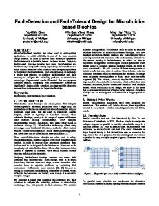
A robotic manipulator with two rigid links adapted from Craig [17] is utilized to the FDI system simulation. The system is simulated in MATLAB and the control scheme employed is the computed-torque. The manipulator parameters are showed in the Appendix. The MLP employed to reproduce the system dynamic behavior has only one hidden layer with 13 neurons. For MLP, training trajectories are chosen so that the maximum of the joint positions space must be covered. Measurement noises are added to the joint positions (mean=O and variance=O.005) and joint velocities (mean=O and varianc~0.05).Ten trajectories with 50 samples each (sample rate is 0.015 s) are used to train the MLP. For example, the trained trajectory 1 is from 8 = [S, &IT = [x/6 0ITto 8 = [2d3 7d2IT.Figure 3 shows a robot trajectory.
0.015
4.025' 0
20
40 60 samples
80
I
100
Figure 5. Residual for the fault-free trajectory from e=[7d24 olTto e = [ i m 41~121~. Two faults are considered. In fault 1, joint 1 is locked. The same occurs for joint 2 in fault 2. Figure 6 shows the residual vector generated in a trajectory where fault 1 occurs between samples 10 and 80. The definition of the pattern set that is most significant in the RBFN training is essential to its performance when nontrained trajectories are presented. In this work, 9 trajectories with 40 samples each are selected. These trajectories are presented three times to the RBFN: one in that the fault 1 occurs, one for fault 2, and one for normal operation. The RBFN is trained by the two algorithms described in section 2.2 [is]. For the tests, 17 trajectories are used. The FDI systems detect all faults and only one
Figure 3. Manipulator performing the trajectory from e=[d4 olTto e=[d2 x/4] T.
1608
false alarm occurred for the system using the FS algorithm. For the RR algorithm none false alarm occurred. Figure 7 shows the outputs of the RBFN trained with FS algorithm for the residual vector of Figure 6 .
Figure 9 shows outputs of the RBFNs trained with RR algorithm for same trajectory and Figure 10 shows fault 1 isolation. Observe that the output signals are smoother. 1.5 output 1
output 2
IW I
O
0.5
I''
-1 0
samples
20
40
60
IO
80
sampIes
Figure 6. Residual in the trajectory from 0=[7d24 0ITto e=[13d24 d2ITwith fault 1 occurringbetween the samples 10 and 80.
Figure 9. RBFN outputs trained with the RR algorithm for the trajectory from 0=[7d24 0ITto 0=[13d24 d2IT with fault 1 occurring between the samples 10 and 80.
fdt 1
operation nitbut
fault 1 L 0
20
-LO
80
40 60 samples
0
-
I 0
40
60
80
0
The FDI system proposed here presents good results when it is applied to a two link planar robotic manipulator. The great attractive of this propose is that according to the tests, FDI system can detect and isolate faults that occur in trajectories that have not been presented before. The MLP reproduces the manipulator dynamic behavior in a fault free case, generally with a small residual signal. RBFN trained with the RR algorithm presented smoother output signals compared to those obtained by RBFN trained with FS algorithm. This occurred because small weights have been employed to produce smoothness in the output function. Large weights are generally employed to produce roughness in the output function. However, the RR algorithm has a higher computational effort than the FS algorithm. The fixing of the matrix R (defines the receptive field size) is important to RBFN performance. If, for example, in RBFN trained with FS a very large
fadtl
I 20
80
6. Conclusions
operation nithorn fault 1
'
60
Figure 10. Fault 1 isolation for RBF trained with RR algorithm (solid line) and real fault 1 (dashed line).
Applying the fault criteria described in last section, the isolation of the fault 1 to this trajectory is showed in Figure 8.
-
40
samples
I00
Figure 7. RBFN outputs trained with FS algorithm for the trajectory from 0=[7d24 0ITto e=[13d24 7r/2ITwith fault 1 occurring between the samples 10 and 80.
1-
20
100
samples
Figure 8. Fault 1 isolation for Rl3F trained with FS algorithm (solid line) and real fault 1 (dashed line).
1609
[12] Chen, S., Cowan, C. F. N. and Grant, P. M. (1991). “Orthogonal least squares learning algorithm for radial basis function networks”, IEEE Trans. on Neural Networks, v.2, 2, pp.302-309. [13] Visinsky, M. L., Cavallaro, J. R. and Walker, 1. D. (1994). “Robotic fault detection and fault tolerance: a survey”, Reliability Eng. and Syst. Safety, 46, pp. 139-158. [14] Visinsky, M. L., Cavallaro, J. R. and Walker, I. D. (1995). “A dynamic fault tolerance framework for remote robots”, IEEE Trans. on Robotics and Automation, v. 11, 4, pp.477-490. [15] Schneider, H. and Frank, P. M. (1996). “Observerbased supervision and fault-detection in robots using nonlinear and fuzzy logic residual evaluation”, IEEE Trans. on Control Syst. Tech.,v.4, 3, pp.274-282. [16] Naughton, J. M., Chen, Y. C. and Jiang, J. (1996). “A neural network aplication to fault diagnosis for robotic manipulator”, R o c . of IEEE Int. ConJ on Control Applications, vol. 1, pp.988-1003. [ 171 Craig, J. J. (1988). “Zntroduction to robotics: mechanics and control”, Addison-Wesley. [18] Orr, M. J. L. (1996). “MATLAB routines for subset selection and ridge regression in linear neural networks”, Center for Cognitive Science, Edinburgh University, Scotland, U. K.
receptive field is defined, the algorithm chooses a small set of radial units. The consequence is that RBFN identifies only the patterns in great clustering, misclasslfying the isolated patterns. Otherwise, if the receptive field is little, a large number of radial units is chose and the resulting classification is very dependent of the training set. The FDI system can be extended to robots with a larger number of degrees of freedom (the computation effort should be higher in these cases). However, faults wluch the system shows the same behavior, independent of the number of freedom degrees, the isolation is difficult because the patterns should occupy the same input space regions.
7. References [l] Gertler, J. (1997). “A cautious look at robustness in residual generation”, Proc. of the IFAC Simp. on Fault Detection, Supervision and Safety for Technical Processes, Kingston Upon Hull, U. K., vol. 1, pp. 133-139. [2] Patton, R. J., Frank, P. M. e Clark, R. N. (1989). ‘