Fault detection in nonlinear systems: An observer-based approach

Fault detection in nonlinear systems: An observer-based approach

Von der der Fakult¨ at f¨ ur Ingenieurwissenschaften der Universit¨ at Duisburg-Essen zur Erlangung des akademischen Grades eines

Doktor-Ingenieurs (Dr.-Ing.) genehmigte Dissertation

von

Muhammad Abid aus I. R. Pakistan

1. Gutachter: Prof. Dr.-Ing. Steven X. Ding 2. Gutachter: Prof. Dr. Michael Kinnaert

Tag der m¨ undlichen Pr¨ ufung: July 16, 2010

Acknowledgments

All praise to Allah who created me, gifted me with a healthy body and brain to work and think and provided me with the opportunities to excel in the life. This work is carried out during my stay at the Institute of Automatic Control and Complex Systems (AKS), University of Duisburg-Essen for acquiring my Ph.D degree. I owe my deepest gratitude to Prof. Dr.-Ing. Steven X. Ding who let me the opportunity to join this excellent institute. His perpetual encouragement, guidance and support enabled me to complete the work. I am also grateful to Prof. Dr. Michel Kinnaert for his interest in my work and his suggestions, corrections and constructive comments. I would like to acknowledge my group mates M.Sc. Abdul Qayyum Khan and M.Sc. Wei Chen for their support and long hour discussions. I am obliged to my senior colleague Dr.-Ing. Ibrahim Al-Salami who not only helped me in research but also in solving social problems during my initial days in Duisburg. I am also indebted to my lab mates for their discussions and creating an inspiring and friendly atmosphere in the lab. Many thanks to to all my colleagues at AKS for their suggestions, comments and support during my research at the institute. I would like to thank my wife for her cooperation and to my parents for their love and affection which helped me to withstand all the difficult stages in my life. Finally, I wish to acknowledge Higher Education Commission (HEC) of Pakistan and German Academic Exchange Program (DAAD) for providing me financial assistance to carry out this research. Muhammad Abid Duisburg, July 16, 2010

iii

To my parents

iv

Contents

Abbreviations and notations

vii

Abstract

ix

1 Introduction 1.1 Motivations . . . . . . . . . . . . . . . . . . . . . . . . . . . . . . . . . . . . . . . 1.2 Objectives . . . . . . . . . . . . . . . . . . . . . . . . . . . . . . . . . . . . . . . . 1.3 Outline and contribution of the thesis . . . . . . . . . . . . . . . . . . . . . . .

1 1 4 5

2 Background and state of the art 2.1 Some basic concepts . . . . . . . . . . . . . . . . . . 2.1.1 Types of faults . . . . . . . . . . . . . . . . . 2.1.2 Desired features of fault detection schemes 2.2 Classification of fault detection schemes . . . . . . 2.2.1 Plausibility test . . . . . . . . . . . . . . . . 2.2.2 Signal-based fault detection . . . . . . . . . 2.2.3 Model-based fault detection . . . . . . . . . 2.3 A comparison of different fault detection methods 2.4 State of the art nonlinear FD techniques . . . . . . 2.4.1 Observer-based residual generation . . . . . 2.4.2 Residual evaluation methods . . . . . . . . 2.5 Summary . . . . . . . . . . . . . . . . . . . . . . . .

. . . . . . . . . . . .

. . . . . . . . . . . .

. . . . . . . . . . . .

. . . . . . . . . . . .

. . . . . . . . . . . .

. . . . . . . . . . . .

. . . . . . . . . . . .

. . . . . . . . . . . .

. . . . . . . . . . . .

. . . . . . . . . . . .

. . . . . . . . . . . .

. . . . . . . . . . . .

9 9 10 11 12 13 13 14 18 18 19 27 30

3 Residual generation with H− , H∞ and H− /H∞ optimizations 3.1 Problem formulation . . . . . . . . . . . . . . . . . . . . . . . 3.2 H− fault sensitive FDF . . . . . . . . . . . . . . . . . . . . . 3.3 H∞ disturbance attenuating FDF . . . . . . . . . . . . . . 3.4 H− /H∞ multi-objective FDF . . . . . . . . . . . . . . . . . . 3.5 An example . . . . . . . . . . . . . . . . . . . . . . . . . . . . 3.6 Summary . . . . . . . . . . . . . . . . . . . . . . . . . . . . .

. . . . . .

. . . . . .

. . . . . .

. . . . . .

. . . . . .

. . . . . .

. . . . . .

. . . . . .

. . . . . .

. . . . . .

. . . . . .

31 35 37 42 48 51 55

. . . . . . . . . . . .

. . . . . . . . . . . .

. . . . . . . . . . . .

. . . . . . . . . . . .

4 Dynamic threshold computation 57 4.1 Problem formulation . . . . . . . . . . . . . . . . . . . . . . . . . . . . . . . . . . 58 4.2 Preliminaries and notations . . . . . . . . . . . . . . . . . . . . . . . . . . . . . . 60 4.3 Dynamic threshold generation . . . . . . . . . . . . . . . . . . . . . . . . . . . . 61

v

Contents 4.4 4.5

An example . . . . . . . . . . . . . . . . . . . . . . . . . . . . . . . . . . . . . . . 64 Summary . . . . . . . . . . . . . . . . . . . . . . . . . . . . . . . . . . . . . . . . 65

5 Optimal trade-off design using post-filter and threshold 5.1 Preliminaries . . . . . . . . . . . . . . . . . . . . . . . . . 5.2 Problem formulation . . . . . . . . . . . . . . . . . . . . . 5.3 Post-filter design . . . . . . . . . . . . . . . . . . . . . . . 5.4 Threshold selection . . . . . . . . . . . . . . . . . . . . . . 5.5 The relationship with optimal residual generators . . . 5.6 An Example . . . . . . . . . . . . . . . . . . . . . . . . . . 5.7 Summary . . . . . . . . . . . . . . . . . . . . . . . . . . . 6 Application to the three tank benchmark 6.1 Description of the three tank system . . . . . . . . . 6.2 Modeling of the three tank system . . . . . . . . . . 6.3 Optimal trade-off design for the three tank system . 6.3.1 Solving PMax-SDF for three tank system . . 6.3.2 Simulation results . . . . . . . . . . . . . . . . 6.3.3 Solving PMin-SDFA for three tank system . 6.4 Summary . . . . . . . . . . . . . . . . . . . . . . . . .

. . . . . . .

. . . . . . .

. . . . . . . . . . . . . .

. . . . . . . . . . . . . .

. . . . . . . . . . . . . .

. . . . . . . . . . . . . .

. . . . . . . . . . . . . .

. . . . . . . . . . . . . .

. . . . . . . . . . . . . .

. . . . . . . . . . . . . .

. . . . . . . . . . . . . .

. . . . . . . . . . . . . .

. . . . . . . . . . . . . .

. . . . . . . . . . . . . .

. . . . . . .

69 71 74 76 79 80 82 86

. . . . . . .

87 88 89 90 91 93 103 106

7 Conclusions and future directions 107 7.1 Conclusions . . . . . . . . . . . . . . . . . . . . . . . . . . . . . . . . . . . . . . . 107 7.2 Future directions . . . . . . . . . . . . . . . . . . . . . . . . . . . . . . . . . . . . 109 A Two-players zero sum differential game

111

B Matrix Calculus

113

C Solution of Hamilton-Jacobi equations (inequalities) 115 C.1 Approach proposed by Aliyu . . . . . . . . . . . . . . . . . . . . . . . . . . . . . 115 C.2 Approach proposed by Wise . . . . . . . . . . . . . . . . . . . . . . . . . . . . . 116 Bibliography

vi

119

Abbreviations and notations

Abbreviations Abbreviation

Meaning

FAR FD FDF FDI FDR HJ HJE HJI HOT inf LTI LMI min RMS SDF SDFA sup

false alarm rate fault detection fault detection filter fault detection and isolation fault detection rate Hamilton-Jacobi Hamilton-Jacobi equation Hamilton-Jacobi-Isaacs higher order terms infimum linear time invariant linear matrix inequality minimum root mean square set of detectable fault set of disturbances that cause false alarms supremum

Notations Symbol

Description

= ≠ ≜ ∈ ⊆ γ

equal to not equal to equal by definition belongs to is subset of Lipschitz constant

vii

Abbreviations and notations t ⇒ ⊗ δd δf,min Σ Σ−1 DΣ ∣⋅∣

element-wise less than or equal to implies Kroneker product end of proof upper bound on L2 norm of disturbance the smallest size of fault to be detected a nonlinear system inverse of a nonlinear system Fréchet derivative of Σ absolute value of a scaler, element-wise absolute value of a vector or matrix ∥⋅∥− H− index for a systems ∥⋅∥∞ L∞ norm of a signal or H∞ norm of a system ∥⋅∥2 L2 -norm of a signal σ(⋅) upper principal gain, maximum singular value lower principal gain, minimum singular value σ(⋅) ∂a partial derivative of a vector a w.r.t. a vector x ∂x T a transpose of a vector a T A transpose of a matrix A A−1 inverse of a matrix A A > 0(A ≥ 0) the symmetric matrix A is positive (semi) definite A < 0(A ≤ 0) the symmetric matrix A is negative (semi) definite f fault vector, the time argument is omitted d unknown input vector, the time argument is omitted D+ generalized or pseudo inverse of D In identity matrix of dimensions n × n In×m identity matrix of dimensions n × m Jth threshold L observer (filter) gain matrix On zero matrix of dimensions n × n On×m zero matrix of dimensions n × m n R space of real valued n-dimensional vector Rn×m space of real valued n × m matrices r residual signal, the time argument is omitted r˜ modified residual signal Vx row vector containing the partial derivative of scaler function V w.r.t. a vector x Vxx second partial derivative of scaler function V w.r.t. a vector x Vt partial derivative of scaler function V w.r.t. a scalar t u input vector, the time argument is omitted x, ξ state vector, the time argument is omitted xˆ estimation of the state vector x y output vector, the time argument is omitted yˆ estimation of the output vector y

viii

Abstract

An un-permitted deviation of at least one characteristic property or parameter of a system from standard condition is referred as a fault. Faults result in reduced efficiency of the system, reduced quality of the product, and sometimes complete breakdown of the process. This not only causes economic losses but may also result in fatalities. An early detection of faults can assist to avert these losses. Therefore, fault detection and process monitoring is becoming an essential part of modern control systems. Fault detection in linear dynamical systems has been extensively studied and well established techniques exist in the literature. However, fault detection for nonlinear dynamical systems is yet an active field of research. This work is motivated by the fact that most of real systems are nonlinear in nature and there is a need to develop fault detection techniques for nonlinear systems. Observerbased methods for fault detection have proven to be among the most capable approaches, therefore, this research is focused towards these methods. The first step in observer-based fault detection is to generate a symptom signal, called the residual signal, which carries the information of faults. This is done by comparing the measurements from the process to their estimates generated by an observer (filter). It is desired that the residual signal is sensitive to faults and robust against disturbances. This research presents new methods for designing observer (filter) to generate residual signal which is sensitive to faults and robust against disturbances. Three types of filters are proposed in this dissertation; these include a fault sensitive filter, disturbance attenuating filter, and a filter to achieve simultaneous attenuation of disturbances and amplification of faults. Despite the disturbance attenuation property of the proposed filters, the residual signal is not completely decoupled from the effect of disturbances and uncertainties. Therefore, a threshold is needed to care for the effect of disturbances and uncertainties. Selection of threshold plays an important role in the performance of the fault detection system. If it is selected too high, some faults will not be detected. Conversely, if it is selected too low, disturbances and uncertainties will result in false alarms. This research presents a new method to determine the threshold to avoid false-alarms and to minimize missed-detections. A threshold generator is proposed which is itself a dynamic system and produces a variable threshold. This threshold changes with the effects of uncertainties and disturbances and fits more tightly to the fault-free residual signal and, hence, the performance of fault detection system is improved. In addition to the residual generation stage, the efficiency of a fault detection system can also be optimized by post-filtering. A further contribution of this research is in proposing

ix

Abstract a post-filter which operates on the residual signal to generate a modified residual signal. This modified residual signal is simultaneously sensitive to faults and robust against disturbances. Together with this post-filter, a strategy is adopted to select a threshold which maximizes the fault detectability and minimizes the number of false-alarms.

x

Chapter

1

Introduction This chapter gives a brief description of the motivations and objectives of this study. The outline of the dissertation and its contribution are also presented in this chapter.

1.1 Motivations The topic of research in this dissertation is observer-based fault detection in nonlinear systems. The motivations of carrying out this study can be elucidated by the following three questions: (1) Why fault detection? (2) Why observer-based methods? and (3) Why nonlinear systems? These questions are answered below. Why fault detection? Due to increasing demand in high degree of sophistication and automation, there is an increasing trend in the complexity of technical processes. With increased complexity, the probability of occurrence of faults is also increased. Faults can occur in the process components, sensors or actuators, for example, short circuiting or overheating of electrical components, breakage in bearings due to mechanical stresses, leakages in pipes, sticking of valves, cracks in tanks, drifting of sensors etc. Faults can cause the process to operate far away from the optimal operating points and hence, can reduce the efficiency of the process, quality of the product and if grown large enough, may result in complete failure of the process which requires additional costs for maintenance. Vedam and Venkatasubramanian [1] claim that only in US petrochemical industry, 20 billion dollars per year is lost due to poor abnormal situation management. In safetycritical processes such as aircrafts, nuclear reactors etc., faults may result in fatalities, a few incidents are listed below: ● Boeing 747-200F lost both engines on taking off from Schiphol Airport in Amsterdam. After 15 minutes, the crew lost the control and the plane crashed into a building with a considerable loss of life. Maciejowski [2] has shown that the incident could have been avoided by reconfiguration of the controller. ● The American Airline DC10 crashed at Chigao-O’Hare International Airport. The pilot had the indication of fault only 15 seconds prior to the accident. Later studies showed that the crash could have been avoided [3].

1

1 Introduction ● An explosion happened in a huge nuclear power plant in the town of Chernobyl in 1986. The main cause for this tragedy was the faulty outdated technology and the lack of a fault handling mechanism [4, 5]. ● Due to complete loss of flying surface in tail, Japan Airlines Flight 123 was crashed on 12 August 1984 resulting in 520 casualties [6]. ● In Delta flight 1080 from San Diego to Los Angeles, the elevator became jammed at 19 degrees up and the pilot was given no indication of the failure. However, the pilot manged to reconfigure the lateral control elements and managed to land safely [3, 5, 7]. Timely detection of faults can avoid, or at least, minimize the severity of economic losses and fatalities by reconfiguration of controllers or safely switching off the process for maintenance. For example, the later studies carried out for the above mentioned incidents proved that many incident could have been avoided if there were a suitable monitoring system. Engineers and researchers have realized the usefulness of fault detection and isolation (FDI) and fault tolerant control (FTC) as indicated by several research papers, invited tutorials, plenary talks in well reputed conferences such as ACC, CDC, IFAC SAFEPROCESS, ECC and IFAC World Congress, and research papers in high ranked journals. Why observer-based methods? Fault detection and isolation (FDI) can be achieved by adding either hardware (or physical) redundancy or analytical redundancy in the process. Hardware redundancy means that additional (redundant) components are used in parallel to the process components. If the behavior of a process component is different from that of the redundant component, it gives an indication of the occurrence of a fault. Hardware redundancy has the advantages of high reliability and direct fault isolation but has associated disadvantages of additional cost, additional space required to accommodate the components and additional weight [8–10]. The analytical redundancy based approaches give indication of faults by comparing the measured outputs of the process to their estimations. Analytical redundancy based fault detection algorithms can be implemented on some digital computer and hence avoid the disadvantages related to the hardware redundancy based fault detection techniques. Due to associated advantages, analytical redundancy based approaches are becoming more and more popular. Figure 1.1 depicts the concepts of hardware and analytical redundancy based fault detection, the analytical redundancy based fault detection algorithms can be implemented in the same processor which implements the control algorithms, thus no additional hardware is needed. Among the analytical redundancy based fault detection schemes, analytical model-based techniques use the deepest knowledge of the monitored process and, therefore, are the most capable approaches for fault detection [11, 12]. There are three types of analytical modelbased approaches, these include: the observer-based approach, parity-space approach and the parameter identification approach. In the past few decades, observer-based methods have received considerable interests. There are possibly three reasons for this particular attention to observer-based methods. Firstly, due to associated advantages of observer-based approaches, e.g., quick detection, requiring no excitation signal, possibility of on-line implementation etc. Secondly, other model-based approaches which include parity-space approach and parameter identification approach are, under certain conditions/assumptions,

2

1.1 Motivations

(a) Hardware redundancy

(b) Analytical redundancy

Figure 1.1: Hardware redundancy vs analytical redundancy: (a) shows the hardware redundancy based fault detection, additional redundant components are used to analyze the presence of faults, (b) shows the analytical redundancy based fault detection, FDI algorithms can be implemented in the same processor which implements the control algorithms, thus no additional hardware is needed.

3

1 Introduction a specific form of the observer-based approaches, and thirdly, control engineers are more familiar with the concepts of observer design. Why for nonlinear systems? Fault detection for linear dynamical systems has been well studied and quite a large number of methods exist in literature. One can find a detailed study of these methods in recent books [8, 13–19] and survey papers [9, 11, 20–25]. Recall that most of the systems are nonlinear in nature, one method for fault detection in nonlinear systems is to linearize them at some operating point and use the techniques developed for linear systems. The linearization errors can be modeled as unstructured uncertainties and their effects can be taken care of by utilizing the robust methods [8, 10]. However, if the process has high nonlinearities, or the operating region is too wide, the linearization error will be too large to be handled by the robust linear fault detection techniques. Therefore, there is a need to study fault detection techniques for nonlinear systems. Fault detection in nonlinear dynamical systems is still an active field of research [26–30] and there is enough space for further improvements.

1.2 Objectives The idea of observer-based fault detection is to generate estimations of measured signals using model of the monitored process, and compare the measurements with their estimations to generate a symptom signal, called the residual signal , which carries the information of faults. In ideal situations, when there are no disturbances and modeling uncertainties, the estimations will completely match with the measurements in fault-free case and the residual signal will be zero. Any deviation of residual signal from zero will give an indication of faults. However, the presence of modeling uncertainties and disturbances is inevitable. Therefore, the aim is to design observers such that the affect of disturbances and uncertainties on the residual signal is reduced while the affect of faults is considerably increased. Now, instead of setting deviation of residual from zero as indicator of faults, a threshold which cares for the effect of disturbances and uncertainties, should be selected and if the residual exceeds the selected threshold, it gives an indication of the presence of faults. The selection of threshold plays a very important role in the performance of a fault detection system, if it is selected too low, some of the disturbances and uncertainties will cause the residual to cross the threshold and appear as faults, this is definitely not desired. Conversely, if the threshold is selected too high, some of the faults will not enable the residual to cross the threshold, and hence will remain undetected. One solution is to select, instead of a constant threshold, a variable threshold which changes with the variations in the effects of uncertainties and disturbances on the residual signal, more the affect of uncertainties and disturbances on residual signal, higher is the threshold and vice versa. This can, to a large extent, improve the performance of fault detection system. In brief, the main objectives in the design of a fault detection system are to design an observer such that the residual signal is minimally influenced by disturbances and uncertainties and is maximally influenced by faults, and to select a threshold which is as close to fault-free residual signal as possible. These design objectives have been solved for linear dynamical systems, comprehensive study can be found in recent monograms [8, 13–15]. The objectives of this dissertation is to present techniques for optimal residual generation and threshold computation for nonlinear dynamical systems. These objectives can be summarized in the

4

1.3 Outline and contribution of the thesis following two points 1. Generation discuss the considered, which have

of residual signal sensitive to faults and robust against disturbances. To sensitivity and the robustness level, the worst case situation should be i.e., the faults which have minimum effect on residual and disturbances maximum effect on residual should be considered.

2. To avoid too conservative threshold, and hence to improve the performance of fault detection system, extension of the concept of variable threshold to nonlinear dynamical systems. If the above mentioned objectives are achieved, faults will be detected more quickly, while there will be less number of false alarms. From the previous statement, one would instantly realize that the real goals of fault detection system are high fault detection rate (FDR) and low false alarm rate (FAR) , optimal residual generation and threshold computation are only tools to achieve these goals. However, high FDR and low FAR are two conflicting goals, therefore, an optimal trade-off should be made between the two. An excellent work to find this optimal trade-off design for linear systems can be found in [13, 31]. The third objective of this dissertation is to solve the optimal trade-off design problem for nonlinear systems, which is summarized in the following point 3. Proposing a strategy for nonlinear systems which achieves an optimal trade-off between high fault detection rate and low false alarm rate.

1.3 Outline and contribution of the thesis This thesis is divide into seven chapters. The first and the second chapters serve as introductory material. The rest of the chapters summarize the contribution and research results of this study. The first chapter describes motivations, objectives and contribution of the thesis. Chapter 2 gives an overview of fault detection and isolation (FDI) and presents some existing methods for fault detection in nonlinear systems. It begins with the definitions of basic concepts such as faults, failures, fault detection etc. A classification of fault detection techniques, with a brief discussion on each approach, is also presented in this chapter. An appropriate attention is paid to observer-based methods, their robustness and sensitivity issues are elaborated. The chapter also presents fault detection methods for nonlinear systems, most commonly used observers for fault detection in nonlinear systems are described in a bit details. State of the art methods for residual evaluation in nonlinear systems are also presented. Residual generation is the first step in an observer-based fault detection scheme. It is desired that the residual signal should be sensitive to faults and robust against disturbances. Over the past, H∞ norm and H− index have been used to measure the disturbance attenuation and fault sensitivity property of residual generator. Based on the standard tools from game theory, Chapter 3 presents approaches for designing H− fault sensitive residual generator, H∞ disturbance attenuating residual generator and H− /H∞ multi-objective residual generator for nonlinear systems. The chapter begins with some examples introducing concepts of H∞ norm and H− index and their significance in fault detection system design. Then sufficient conditions for H− fault sensitivity of residual signal are derived. A 5

1 Introduction delicate difference between H∞ filtering problem and H∞ fault detection filtering problem is explained, an example is provided to highlight the difference. It is explicated that although the H∞ filtering problem has been extensively studied, H∞ fault detection filtering problem for nonlinear systems has not been discussed. Sufficient conditions for H∞ fault detection filtering problem are derived for nonlinear systems. Simultaneous attenuation of disturbances and amplification of faults is desired feature of a residual generator, therefore, the H− /H∞ multi-objective fault detection filtering problem is discussed. In all the three filters, both finite horizon and infinite horizon cases are handled. The proposed methods are demonstrated by simulation examples. With the fault detection filters mentioned above, the effect of disturbances on the residual signal is not completely eliminated, therefore, there is a need to use a threshold. Selection of threshold is significantly important in the design of a fault detection system, preferably a variable threshold can achieve a better performance. Chapter 4 begins with explaining the concept of variable thresholds. Based on the recently proposed approach of dynamic threshold generation for linear systems, Chapter 4 presents an approach to generate dynamic threshold for a class of nonlinear systems. A dynamic upper bound on the modulus of error dynamics is obtained which is used to generate a dynamic threshold. With a simulation example of a simple second order system, it is demonstrated that the proposed method of dynamic threshold generation can successfully avoid false alarms and can detect small faults. The residual generation methods presented in Chapter 3 and threshold selection technique presented in Chapter 4 are tools to achieve a trade-off between high FDR and low FAR. This optimal trade-off can also be reached by designing a dynamic post-filter and a determining a threshold. With the assumption that a stable residual generator is available, Chapter 5 presents an approach to design a post-filter and determine a threshold to attain an optimal trade-off between high FDR and low FAR. The optimal trade-off design problem is formulated into two optimization problems; these are the maximization of fault detectability for an allowed FAR and the minimization of false alarms for a required FDR. For the first optimization problem, a threshold is selected which guarantees that the FAR is not more than the allowed one. Then based on the selected threshold and utilizing the factorization approach, a post-filter is proposed which maximizes fault detectability. Similarly for the second optimization problem, a threshold is selected to ensure the required FAR and the post-filter minimizes the number of false alarms. Furthermore, it is demonstrated that after using the post-filer, which acts on the residual signal to generate a modified residual signal, the modified residual signal is sensitive to faults and robust against disturbances, i.e. the proposed post-filter also gives optimization in the sense of H− /H∞ optimization. A simple example is provided to illustrate the proposed methods and to show its effectiveness. Chapter 6 gives the application of the optimal trade-off design method developed in Chapter 5 to the three tank system. The three tank system has high nonlinearities and is, therefore, widely used as a benchmark to test nonlinear control and FDI algorithms. After describing the three tank system, a fault detection filter is used to generate residual signal. Then a post-filter is designed and threshold is computed to give and optimal trade-off between high FDR and low FAR. The simulation results are presented which show that all the faults including sensor faults, actuator faults and component faults are successfully detected. Both abrupt and incipient fault situations are presented. The concluding remarks of this research and some future recommendations for possible

6

1.3 Outline and contribution of the thesis extension of the work are presented in the last chapter.

7

Chapter

2

Background and state of the art This chapter introduces to the basic concepts in fault detection and isolation (FDI) and presents some existing methods for fault detection in nonlinear systems. Fundamental concepts, such as faults, failures, fault detection, fault isolation etc. are defined. Different types of faults and their effects on the performance of processes are explained. Several methods for fault detection exist in literature; a widely accepted classification of these methods is presented with a particular focus on the model-based fault detection techniques. Observer-based fault detection in nonlinear systems is of major interest in this thesis, therefore, state of the art observer-based residual generation methods for nonlinear systems are presented in a bit details. Most commonly used evaluation functions and threshold selection approaches are described.

2.1 Some basic concepts The terminologies used in FDI has been fairly standardized after the suggestions from SAFEPROCESS Technical Committee [25]. Throughout the text a fault means an unpermitted deviation of at least one characteristic property or parameter of a system from the acceptable/usual/standard condition. A very related term is failure which is a permanent interruption of the system’s ability to perform a required function under specified operating conditions. There is a slight difference between fault and failure, failure means complete breakdown of a component, whereas fault is only deviation from normal characteristics. As far as detection is concerned, faults and failures can be treated alike. In sequel, we will use the term fault to encompass failure as well. Faults can be described as external inputs or parameter deviations which change the behavior of the process. Like faults, disturbances and uncertainties can also be modeled as external inputs. Furthermore, disturbances and uncertainties have effects on the process similar to that of faults. But as compared to faults, disturbances are unavoidable and are present even during the normal operation of the process. Moreover, the controller is designed so that it can perform well in the presence of disturbances. Faults, on the other hand, are more severe changes and their affects can not be overcome by a fixed controller and, therefore, must be detected. The purpose of fault diagnosis is to detect faults and to determine their locations and

9

2 Background and state of the art

Figure 2.1: Representation of different kinds of external inputs to a system, including faults, disturbances and parameter variations significance. The procedure of fault diagnosis consists of three steps namely fault detection, fault isolation and fault identification. Fault detection (FD) is the process of determining the presence of faults and the time of their occurrence. The function of fault isolation is to exactly locate the reason or the origin of fault. Once the fault has been detected and isolated, the step of fault identification starts that aims to find an approximate time behavior of the fault. The conditions for the isolation of faults are quite harder and that of fault identification or even more stringent (see [13, Chapter 4]) which makes it, in most situations, impossible to isolate and identify the faults. The scope of the thesis is limited to the detection of faults.

2.1.1 Types of faults Fault in a system is an external input that causes a deviation from the normal behavior of the system. Faults can occur in the actuators, process components or the sensors as shown in Figure 2.1, and are categorized accordingly. Each of these faults and their effects are briefly described below. Component faults These are the faults which appear in the components of plant. Component faults alter the physical parameters of the plant which, in turn, results in change of its dynamical properties. The common reason for these faults is usually wear and tear, aging of components etc. Some examples of component faults are leakages in tanks, breakages or cracks in gearbox system, change in friction due to lubricant deterioration etc. Component faults may result in instability of the process, therefore, it is extremely important to detect these faults. Actuator faults Actuators are needed to transform control signals into proper actuation signals such as torques and forces to drive the system. A fault in an actuator may result in higher energy consumption to total loss of control [28]. Examples of actuator faults include stuck-up of control valves, faults in pumps, motors etc. Some common actuator faults in servomotors

10

2.1 Some basic concepts

(a)

(b)

(c)

(d)

Figure 2.2: Graphical representation of common types of actuator faults in servomotors [32]. Dotted lines show the desired value of actuator and the solid lines show actual value. (a) floating around trim, (b) lock-in-place, (c) hard-over failure and (d) loss of effectiveness are lock-in-place, float around trim, hard-over failure and loss of effectiveness [28, 32] as shown in Figure 2.2. Sensor faults In closed loop systems, the measurements obtained by sensors are used to generate the control inputs and any fault in sensors can cause operating points that are far from the optimal ones [14]. This results in degradation in the performance of the system. It is therefore, very important to detect these faults. Typical examples of sensor faults are: bias, drift, performance degradation (or loss of accuracy), sensor freezing and calibration error [28, 32, 33] as illustrated in Figure 2.3. Faults can also be categorized according to whether these have developed slowly in the system (Incipient faults) , arisen suddenly like a step change (Abrupt faults) or occurred in discrete intervals (Intermittent faults) as shown in Figure 2.4. Abrupt faults have more severe affects and may result in damage of equipments. However, fortunately abrupt faults are easier to detect. Incipient faults grow slowly and result in degradation of equipments. Their slowly changing behavior makes it difficult to detect them. Faults may also be classified into additive faults and multiplicative faults according to the way in which these are modeled. Actuator and sensor faults are more easily modeled as additive faults, whereas component faults are modeled as multiplicative faults.

2.1.2 Desired features of fault detection schemes Advanced methods of fault detection should satisfy the following requirements [15] ● early detection of abrupt and incipient faults

11


(a)

(b)

(d)

(c)

(e)

Figure 2.3: Graphical depiction of different kinds of sensor faults [33]. Solid lines show the actual values whereas the dotted lines show the measured values. (a) Bias, (b) Drift, (c) Loss of accuracy, (d) Freezing and (e) Calibration error

(a) Abrupt fault

(b) Incipient fault

(c) Intermittent fault

Figure 2.4: Graphical illustration of abrupt, incipient and intermittent faults occurring at time tf ● detection of actuator, component and sensor faults ● detection of faults in closed loop ● supervision of processes in transient states Other than the above mentioned features, a fault detection technique should consume less computational cost so that on-line implementation is easily achieved. Furthermore, the design procedure should be simple.

2.2 Classification of fault detection schemes The importance of fault detection has been realized since the invention of machines. The earliest way of detecting faults was biological senses, such as looking for changes in color and shape, listening to sounds unusual in pitch and loudness, touching to feel heat or vibration, and smelling for fumes because of leakage or overheating [16]. However, with industrial

12

2.2 Classification of fault detection schemes revolution, there was a need to autonomously detect faults without human intervention. This was to save extra labor, to achieve more precise and quick detection of faults and the fact that some parts or location may not be accessible to, or dangerous for human beings. Classical way of fault detection is by limit checking which is done by setting an upper and lower limit for the measured variables. If the measured variable exceeds the limit, it gives indication of fault. There has to be a compromise in selecting the limit bound; if selected too narrow some fluctuations and disturbances will cause an alarm of fault and if selected too wide, some of the small magnitude faults may not be detected. These methods are suitable for processes with steady state behavior. The advantage of these methods is simplicity and reliability for steady-state situations [15, 34]. The disadvantage of limit checking methods is that faults can be detected only when these grow large enough to cross the limit. This may cause more damage to the process as compared to that if it was detected earlier and suitable remedies had been taken. Another disadvantage is that these methods fail when the monitored process has dynamic properties or the operating points are changing rapidly. Therefore advanced methods of supervision must be used. These methods can be classified into i) Plausibility test, ii) Signal-based methods and iii) Model-based methods. These are briefly described in the following subsections.

2.2.1 Plausibility test The idea is based on checking the plausibility of measured values. This means that the measurements are compared with their rough behavior under normal operation, for example, the sign and size of the measurements. The plausibility test can be implemented by simple logical gates. It has the drawback that it is less efficient in detecting faults and becomes impossible in complex plants.

2.2.2 Signal-based fault detection In signal-based approaches, one gets the information of faults by collecting some properties of the measured signals. Examples of these properties are the magnitudes of the time function, trend checking from the derivative, mean and variance, spectral power densities, correlation coefficients, etc., of the measured signals. Figure 2.5 shows the conceptual diagram for signal-based fault detection schemes. Limit checking of absolute value of the measurements and the limit checking of derivative (trend) of the measurements are the two most simple and widely used approaches for fault detection. In limit checking of absolute value of the measurements, suitable upper and lower limits are set based on the knowledge of the plant, and if the magnitude of the measurement crosses the limit, it gives an indication of a fault, i.e., Ymin ≤ y(t) ≤ Ymax ⇒ fault-free y(t) < Ymin or y(t) > Ymax ⇒ faulty Similarly, in limit checking of the trend of the measurements, if the derivative of the measurements crosses the pre-defined upper and lower limits, a fault alarm is released, i.e., Y˙ min ≤ y(t) ˙ ≤ Y˙ max ⇒ fault-free y(t) ˙ < Y˙ min or y(t) ˙ > Y˙ max ⇒ faulty

13


Figure 2.5: Schematic diagram of signal-based fault detection scheme Limit checking approach is simple and can be easily implemented. However, the drawback is that fault can only be detected when it grows enough to cross the limits. Moreover, these approaches are not suitable for the dynamic systems with transient behavior.

2.2.3 Model-based fault detection The idea of model-based fault detection schemes is to compare the behavior of actual process to that of the nominal fault-free model of the process driven by the same input. Modelbased approaches are more powerful than the signal processing-based approaches [11, 12], because these use more information about the process. Figure 2.6 shows the schematic diagram of a model-based fault detection scheme. It consists of two main stages; residual generation and residual evaluation. The objective of residual generation is to produce a signal, called residual signal, by comparing the measurements with their estimates and the purpose of residual evaluation is to inspect the residual signal for possible presence of faults. Based on the model used for the purpose of residual generation, model-based fault detection schemes can further be divided into two categories. The model can be an analytical model represented by set of differential equations or it can be knowledge-based model represented by, for example, neural networks, petri nets, experts systems, fuzzy rules etc. Knowledge-based model approaches do not need full analytical modeling, therefore, are more suitable in information-poor systems or in situations where the mathematical model of the process is difficult to obtain or is too complex. This is the case, for example, in chemical processes which are difficult to model analytically. A comprehensive study of these methods can be found in survey papers [11, 35–38] and recent books [17, 38]. Recently, hybrid approaches which simultaneously use the mathematical model and neural networks have also been proposed [28]. In analytical model-based approaches, residual signal is generated using the mathematical model of the system. The most commonly used analytical model-based approaches for residual generation include i) Observer-based approach, ii) Parity space approach and iii) Parameter estimation-based approach, these are described below.

14

2.2 Classification of fault detection schemes

Figure 2.6: Schematic diagram of model-based fault detection schemes

Figure 2.7: Schematic diagram of observer-based residual generator Observer-based approach In observer-based approaches, residual signal is generated by comparing measurements from process with their estimates generated by an observer (a filter). It should be noted that there is a difference between observers used for control purposes and observers for FD. The observers needed for control are state observers, i.e., they estimate states which are not measured. In contrary, the observers needed for FD are output observer, i.e., these observers generate estimation of the measurements. A special form is the fault detection filter, which generates estimation of all the states, irrespective of whether they are measured or not. In this case, these can be used both for control and FDI. Figure 2.7 shows the schematic diagram of an observer-based residual generation scheme. The idea of using observers for residual generation goes back to 1970s when Beard proposed a detection filter which was later modified by Jones to the so called Beard-Jones detection filter. In parallel to the Beard-Jones detection filter, Kalman filter was used in stochastic setting.

15

2 Background and state of the art The robustness of residual signal against unknown inputs has been widely discussed in literature and several approaches have been proposed to tackle this problem, a survey of these approaches can be found in [39]. The first attempt to improve the robustness of observer-based instrument fault detection scheme was made by [40]. Robust fault detection using unknown input observers was a focus of research in 1980’s. With a pioneering work of [41], a considerable contribution was made in literature by [42–45]. The idea is to completely decouple the state estimation from unknown inputs (disturbances) using the information of the unknown input distribution matrix. If the states are decoupled from the unknown inputs, residual is also independent. A related approach for robust residual generation is use of eigenstructure approach which also decouples residual from unknown inputs. The existence conditions for the eigenstructure assignment approach are more relaxed compared to unknown input observers. In this approach, instead of decoupling state estimations from unknown inputs, the residual signal is made independent of unknown inputs. The approach was initially proposed in [46] and further developments were made in [47, 48]. Another approach for disturbance decoupling was proposed in [49] which involves geometric approach for decoupling the effect of disturbance. Unknown input observers, eigenstructure assignment approach and the geometric approach are all based upon eliminating the effect of disturbance. However, these approaches can not properly handle modeling uncertainties. One way to handle the uncertainties is to model them as external unknown inputs and then utilize the disturbance decoupling approaches. The existence conditions for disturbance decoupling approaches are quite stringent which restricts their application. Furthermore, if the fault lies in the same space as the disturbances, its effect on the residual is also decoupled and cannot be detected. Therefore, instead of completely decoupling unknown inputs, much focus has also been paid to design observers which attenuate the effect of unknown inputs and amplify the effect of faults on the residual signal. Following the standard results from control theory, several approaches [43, 50, 51] were proposed utilizing the H∞ , H2 indices to design observer so as to attenuate the effect of disturbance on the residual signal. In parallel to robustness problem, much of attention is also paid to fault sensitivity problems [52–55]. With simultaneous consideration to robustness and sensitivity proposed in [56], there were a series of articles which solved the sensitivity and robustness problem and LMI solutions were presented to solve H− /H∞ multi-objective optimization [53, 55, 57–60]. The unified solution was presented in [61, 62] which gives a simultaneous solution of the multi-objective Hi /H∞ optimization and involves less computations. A comprehensive study of the unified approach can be found in [13]. Observer-based approach for fault detection in nonlinear systems is the main interest of this thesis. A survey of some observer-based techniques for residual generation in nonlinear systems will be presented in Section 2.4.1. Parity space approach The parity space approach uses the check of parity of mathematical equations of the system by using the measurements. Chow and Willsky [63] first proposed parity equations for state space model of the system, later contributions were made using the transfer functions in [64–66]. Figure 2.8 shows the configuration of parity space-based residual gneration [11]. Parity space approach and observer-based approach are similar as shown in [12, 67, 68] and there exists a one-to-one mapping between the design parameters of observer and

16

2.2 Classification of fault detection schemes

Figure 2.8: Schematic diagram of parity space approach for residual generator

parity relation based residual generator. Two theorems are presented in [13] that show how to calculate parity vector corresponding to observer-based residual generator and vice versa. Thus we can design residual generator in parity space and then can transform the parity vector into diagnostic observer parameters for on-line implementation. The implementation of the parity relation based residual generator uses a non-recursive form, while the observer-based residual generator represents a recursive form. Thus it is usual to design in parity space and to realize in observer-based structure. Parity relation based fault detection schemes have also been utilized for nonlinear systems. Krishnaswami and Rizzoni [69] presented a parity space approach based on the inverse model of input output nonlinear systems. Recently, [70, 71] generalized the parity space approach for linear systems to nonlinear systems described by TS fuzzy models. A comprehensive study of parity space approach for nonlinear processes can be found in [15]. For multi-input single-output nonlinear systems, the relationship between the parity relations and high gain observers has been shown in [72, 73].

Parameter estimation based approach The parameter estimation approach for fault detection was first proposed in [74–76] and is based on the assumption that the faults are reflected in the physical parameters of systems. With this assumption, parameters of system are estimated on-line repeatedly, if there is a discrepancy in the estimated parameters and the actual parameters, it gives indication of faults. An advantage of parameter estimation approach is that with only one input and one output signal, several parameters can be estimated which give a detailed picture on internal process quantities [15]. Another advantage of the method is that it yields the size of the deviations which is important for fault analysis [11]. Parameter estimation based approach is useful for component fault detection, although it can also detect sensor and actuator faults. A disadvantage is that an excitation is always needed in order to estimate the parameters which may result in problems if the precess is operating at a stationary points [11]. There are several parameter estimation techniques, among them are methods of least squares (LS), recursive least squares (RLS), extended least squares (ELS), etc. Parameter estimation techniques have also been applied to fault detection in nonlinear systems, study of parameter estimation based fault detection in nonlinear systems can be found in [15] and application to a nonlinear satellite model in [77]. There is a close relationship between parameter identification based fault detection and the observer-based fault detection approach as demonstrated in [78, 79].

17


2.3 A comparison of different fault detection methods It is quite difficult to compare different fault detection schemes. The decision upon which FD method should be used depends on several factors, among them are the availability of mathematical model, information about the process, type of disturbances and uncertainties, nonlinearities, closed loop or open loop etc. For example, in electrical and mechanical systems, it is relatively easy to obtain a mathematical model so analytical model-based approaches are preferred. In contrary, chemical and industrial processes are difficult to model, or even if a mathematical model can be obtained, it is quite complex. In that case, qualitative model-based approaches or signal-based approaches should be applied. Analytical model-based approaches are usually faster and on-line implementation is easier hence more suitable for processes with fast dynamics. Among the analytical model-based approaches, an interesting comparison is presented in [15] which could be used as a guideline for selecting the FD method. Parameter estimation based approaches need only the structure of the process as against parity space approaches and observer-based approaches which need not only the structure of the process but also the parameters. Both the parity space approach and the observer-based approach do not need an input signal change to detect faults whereas parameter estimation approach requires input excitation. To detect multiplicative faults, parameter estimation approach is a better choice as compared to observers and parity equations. Parity space approaches are more sensitive to measurement noise as compared to observer-based approaches and parameter estimation approaches. It is also possible to combine different approaches to collect the advantages of each approach. A few combining strategies are enlisted in [15].

2.4 State of the art nonlinear FD techniques Most of the real systems are nonlinear in nature. One approach for the fault detection of nonlinear systems is to linearize them at operating points and use the well established theory of linear FDI. The effect of linearization errors is handled by applying robust FDI schemes. In certain cases when the linearized model does not deviate too much from the nonlinear model, these approaches can perform well. However, in situations where the monitored process has high nonlinearities, or the operating region of the plant is large enough, linearization about a point may result into high modeling errors. Using the linear model-based approaches will result into high false alarm rate with most of the faults undetected [22]. These limitations of linear FD methods motivated the researchers to study the nonlinear fault detection techniques. Several approaches for fault detection of nonlinear systems have been proposed. These include analytical model-based techniques [8, 80], neural networks [81], fuzzy systems [11], data driven methods [82], statistical techniques etc. Among these techniques, the analytical model-based approaches use the deepest knowledge of the process, and therefore, are the most capable approaches for fault detection provided that the mathematical model of the process is available. Three types of analytical model-based residual generation approaches are classified in the last section, these are the observer-based approach, parity space approach and parameter identification approach. The major focus of this thesis is observer-based approaches because of two reasons. Firstly, it has been shown that parity relations are a special form of observers, called the dead-beat observers (i.e. observers

18

2.4 State of the art nonlinear FD techniques having all the poles at origin). Likewise, parameter identification approaches have much similarities to observer-based approaches. So, it does not cause any loss of generality to focus on observer-based approaches [12]. Secondly, observers are more familiar to the control community as compared to parity relations and parameter identification approaches. In the next subsection, some state of the art methods for observer-based residual generation in nonlinear systems are explained. Residual evaluation techniques will be presented in subsection 2.4.2.

2.4.1 Observer-based residual generation Over the past, several observer-based approaches for residual generation in nonlinear systems have been proposed, see [8, 22, 27, 30, 39, 80, 83] for survey of these approaches. Some of them are described in below: Extended Luenberger observer The Luenberger observer was used for fault detection in linear systems in [84]. For fault detection in nonlinear systems, one can linearize the nonlinear model at an operating point and apply the Luenberger observer. However, if the operating region is too wide, the linearized model will deviate largely from the nonlinear model, particularly, if the system is operating away from the linearizing point. The idea of the extended Luenberger observer is to linearize the model around current estimate of states xˆ(t), instead of a fix point (e.g. x = 0), and then apply the Luenberger observer. Consider, for example, the nonlinear system x˙ = a(x, u), y = c(x, u)

x(0) = x0

Then a nonlinear observer is xˆ˙ = a(ˆ x, u) + L(ˆ x, u)(y − c(ˆ x, u)), yˆ = c(ˆ x, u)

xˆ(0) = xˆ0

where L(ˆ x, u) is the observer gain which is computed at each time instant in such a way that the eigenvalues of ( ∂a(x,u) − L(ˆ x, u) ∂c(x,u) ∂x ∂x ) are stable. The detailed study can be found in [85]. A similar approach for state estimation and its application to fault detection has been proposed in [86]. Because of the requirements of repetitive calculation of observer gain (which means more on-line computations) and the linearization errors, the extended Luenberger observer is rarely used in practice. In stochastic settings, the counterpart of the extended Luenberger observer is the extended Kalman filter (EKF) . Similar to extended Luenberger observer, the basic idea of extended Kalman filter is to linearize the system around the current estimation of states and apply the linear Kalman filter. The Thau observer approach The Thau observer was developed in [87] for the state estimation of a class of nonlinear systems. It has also been applied to fault detection in [88]. The class of nonlinear systems

19

2 Background and state of the art examined in this approach is described by x˙ = Ax + Bu + g(x, u) y = Cx

It is assumed that the pair (C, A) is observable, the nonlinear part g(x, u) is continuously differentiable and satisfies the Lipschitz condition locally, i.e. ∥g(x, u) − g(ˆ x, u)∥ ≤ γ ∥x − xˆ∥ The structure of the Thau observer is given by xˆ˙ = Aˆ x + Bu + g(ˆ x, u) + L(y − yˆ) r = y − C xˆ

and the observer gain L = P −1 C T , P is the solution to the Lyapunov equation AT P + P A − C T C + θP = 0

(2.1)

where θ is a positive parameter which is chosen in such a way that it ensures the solution of the Lyapunov equation (2.1). Nonlinear identity observer approach The nonlinear identity observer was first proposed in [89] for detection and isolation of component faults. Further contributions were presented in [21, 86]. The nonlinear system considered is given as x˙ = a(x, u), y = c(x, u)

x(0) = x0

The nonlinear observer is then given by xˆ˙ = a(ˆ x, u) + L(ˆ x, u)(y − yˆ) r = y − c(ˆ x, u)

Defining the estimation error e = x − xˆ, the error dynamics can be written as e˙ = A(ˆ x, u)e − L(ˆ x, u)C(ˆ x, u)e + HOT r = C(ˆ x, u)e + HOT

where

∂c(x, u) ∂a(x, u) ∣ , C(ˆ x, u) = ∣ ∂x ∂x x=ˆ x x=ˆ x and HOT represents the higher order terms. Neglecting these HOT, the gain matrix L(ˆ x, u) can be found in such a way that the error dynamics are asymptotically stable. In some situations, for example in Lipschitz nonlinear systems, a constant matrix will guarantee the stability[80]. For the case C(x, u) = Cx, the matrix L(ˆ x, u) has the form [80] A(ˆ x, u) =

ˆ x, u)C T Q L(ˆ x, u) = P −1 A(ˆ

20

2.4 State of the art nonlinear FD techniques where the symmetric positive definite matrix P should be such that ∂a(x, u) ∣ 0, M > 0, M > 0 such that, for every t ≥ 0, ǫ ≤ ∣ai (t)∣ ≤ M and ′ ∣ dtd ai (t)∣ ≤ M for i = 1, ⋯, n − 1

then an observer for (2.5) is of the form

xˆ˙ = A(t)ˆ x + ψ(t, u, xˆ) − Λ−1 (t)Sθ−1 C T (C xˆ − y)

where Sθ is the solution of (2.4) and

Λ(t) = diag{1, a1 (t), a1 (t)a2 (t), ⋯, a1 (t)⋯an−1 (t)} Sliding mode observer approach Sliding mode observers have been vastly applied to fault detection in linear systems [99–102] as well as in nonlinear systems [103–107]. The inherent property of sliding mode observers of being robust to uncertainties and disturbances makes them suitable for state estimation and fault detection. Designing a sliding mode observer consists of two steps, construction of a sliding surface and designing a control law which drives the system trajectories to the

23

2 Background and state of the art sliding surface in finite time. As the trajectories reach to the sliding surface, they become insensitive to the external disturbances. In below, we describe the major steps involved in the design of sliding mode observer. The discussion is based on the results from [104]. Consider the class of nonlinear systems described by x˙ = Ax + g(x, u) + Eψ(x, u, t) y = Cx

(2.6)

x ∈ Rn , u ∈ Rm and y ∈ Rp are the sate vector, input vector and the output vector, respectively. A ∈ Rn×n , E ∈ Rn×r , D ∈ Rn×q and C ∈ Rp×n are the constant matrices. The unknown nonlinear term g(x, u) is Lipschitz with respect to x, the unknown nonlinear term ψ(x, u, t) represents the modeling uncertainties and disturbances and is bounded by a known Lipschitz function ξ(x, u, t), i.e., ∥ψ(x, u, t)∥ ≤ ξ(x, u, t)

Under the assumption that rank(C[E D]) = rank([E D]), there exists a coordinate system in which the triple (A, [E D], C) has the following structure ([

0 0 A1 A2 ] , [ (n−p)×r (n−p)×q ] , [ 0p×(n−p) C2 ] , ) A3 A4 E2 D2

where A1 ∈ R(n−p)×(n−p) , C2 ∈ Rp×p are nonsingular. Hence, the system (2.6) can be represented as x˙ 1 = A1 x1 + A2 x2 + g1 (x, u) x˙ 2 = A3 x1 + A4 x2 + g2 (x, u) + E2 ψ(x, u, t) y = C2 x2

(2.7)

If all the invariant zeros of the matrix triple (A, [E D], C) lie in the left half plane, then there exists a matrix L which has the structure L = [L1 0] such that A1 + LA3 is stable. Applying the coordinate transformation z=[

In−p L ]x 0 Ip

to the system (2.7) results into z˙1 = (A1 + LA3 )z1 + (A2 + LA4 − (A1 + LA3 )L) z2 + [In−p L]g(T −1 z, u) z˙2 = A3 z1 + (A4 − A3 L)z2 + g2 (T −1 z, u) + E2 ψ(T −1 z, u, t) y = C2 z2

(2.8)

Then a sliding mode observer for (2.8) is given as zˆ˙1 = (A1 + LA3 )ˆ z1 + (A2 + LA4 − (A1 + LA3 )L)C2−1 y + [In−p L]g(T −1 zˆ, u) zˆ˙2 = A3 zˆ1 + (A4 − A3 L)ˆ z2 − K(y − C2 zˆ2 ) + g2 (T −1 zˆ, u) + ν(t, u, y, yˆ, zˆ) yˆ = C2 zˆ2

24

(2.9)

2.4 State of the art nonlinear FD techniques The gain matrix K is chosen such that C2 (A2 − A3 L)C2−1 + C2 K is symmetric negative definite. The function ν is defined by ν = k(⋅)C2−1

y − yˆ ∥y − yˆ∥

if y − yˆ ≠ 0

(2.10)

where k(⋅) is a positive scalar function to be determined. With the state estimation error defined by e1 = z1 − zˆ1 and ey = y − yˆ = C2 (z2 − zˆ2 ), the motion of estimation error dynamics associated with the the sliding surface defined by

is stable if the matrix inequality

S = {(e1 , ey )∣ey = 0}

1 A¯T P¯ T + P¯ A¯ + P¯ P¯ T + ǫγg2 In−p + αP < 0 ǫ is solvable for P¯ . Where P¯ = P [In−p L], A¯ = [A1 A3 ]T , P > 0, α and ǫ are positive constants and γg is the Lipschitz constant for the g(x, u) with respect to x. The scalar function k(⋅) is chosen to satisfy k(t, u, y, zˆ) ≥ (∥C2 A3 ∥ + ∥C2 ∥ γg + ∥C2 E∥ γξ )wˆ + ∥C2 E2 ∥ ξ(T −1 zˆ, u, t) + ∥C2 D2 ∥ ρ(y, u, t) + η

where η is a positive constant and wˆ is the solution to the differential equation 1 wˆ˙ = − αw(t) ˆ 2 Geometric approach

The nonlinear geometric approach for fault detection, proposed in [108], is nonlinear extension to the detection filter proposed by Massoumnia [109]. The idea is based on constructing a subsystem which is affected by faults and is decoupled from disturbances. This is done by finding an unobservability subspace in which all disturbances are unobservable. Once this subspace has been determined, a simple asymptotic observer is designed for the subsystem, and this guarantees that the disturbances are decoupled. The geometric approach can also be used for fault isolation. In this case all faults, except the one to be isolated, are treated as disturbances and are rendered unobservable to the subsystem. Persis and Isidori [108] proposed recursive algorithm to find the unobservability subspace. The geometric approach suffers from the same disadvantages as the unknown input observer techniques. For certain systems, such an unobservability subspace may not exist or faults may also belong to the same subspace as the disturbances. Game theoretic approach for observer design Game theory has been utilized to design observers for linear [110–112] as well as nonlinear systems [113–118], specifically in the context of fault detection [50, 119, 120]. The advantage of applying game theory is that extreme case scenario can be treated very easily and the H∞ disturbance attenuating observers can be designed for nonlinear systems. Another advantage is that more general class of nonlinear systems can be handled.

25

2 Background and state of the art To design H∞ disturbance attenuation filter using game theory, the fundamental idea is to find out the worst possible disturbance and then to design an observer gain which achieves the desired attenuation of the disturbance. If the designed observer can achieve a desired level of attenuation α to the worst possible disturbance, all other disturbances which are not the worst disturbance will be clearly attenuated more than that attenuation level α. Below we present game theoretic observer for nonlinear systems. It should be noted that this is not a fault detection filter, rather a state estimation filter. The objective to present it here is that our approach presented in Chapter 2 is base on similar ideas. For the class of nonlinear systems described by x˙ = a(x, t) + Ed (x, t)d y = c(x, t) + Fd (x, t)d

which satisfies the following assumptions

● a, Ed and Fd are smooth functions in x for every t, and continuous in t ● a has an equilibrium point x0 , i.e., a(x0 , t) = 0 ∀t

● c(x0 , t) = 0 ∀t

● x0 is asymptotically stable point of f ● Ed (x, t)FdT (x, t) = 0 ∀t

Berman [114] proposed the following observer to ensure the H∞ disturbance attenuation level greater than or equal to α xˆ˙ = a(ˆ x, t) + L(ˆ x, t)[y − c(ˆ x)] yˆ = c(ˆ x, t) The filter gain matrix L(ˆ x, t) is the solution of the following equation where Vxˆ =

∂V ∂x ˆ

Vxˆ L(ˆ x, t) = −2α2 [c(x, t) − c(ˆ x, t)]T (Fd (x, t)FdT (x, t))−1

is the solution of the following partial differential inequality

∂V + Vx a(x, t) + Vxˆ a(ˆ x, t) ∂t − α2 [c(x, t) − c(ˆ x, t)](Fd (x, t)FdT (x, t))−1 [c(x, t) − c(ˆ x, t)] 1 + [c(x, t) − c(ˆ x, t)][c(x, t) − c(ˆ x, t)]T + 2 Vx (Ed (x, t)EdT (x, t))VxT ≤ 0 4α An advantage of the above approach is that more general class of systems can be treated. An associated disadvantage is that the approach is restricted by the demand to solve nonlinear partial differential equation (inequality). Another very interesting approach utilizing the game theory for optimal sensitive fault detection filter design was introduced in [120]. To describe the method, consider a class of nonlinear systems described by x˙ 1 = a1 (x1 , u) + a2 (x1 , u)x2 + Ef (x1 , u)f y1 = c(x1 ) + d1 y2 = x2 + d2

26

2.4 State of the art nonlinear FD techniques It is desired to find a filter such that for some fixed positive number α and a given choice of positive definite matrices Q, M , N , V , Π0 , the cost function t1

x1 )∣2Q + ∣f ∣2N −1 − α2 (∣d2 ∣2N −1 + ∣d1 ∣2V −1 )]dt − ∣x1 (0)∣2α2 Π0 J(f, d1 , d2 ) = ∫ [∣c(x1 ) − c(ˆ

(2.11)

0

is such that

sup inf J(f, d1 , d2 ) ≤ 0

d1 ,d2 f

(2.12)

Based upon the above cost function, the following filter is proposed ∂c (ˆ x1 , t) ( xˆ˙ 1 = a1 (ˆ x1 , u) + a2 (ˆ x1 , u)y2 + 2α2 Yx−1 (ˆ x1 )) V −1 (y1 − c(ˆ x1 )) 1 x1 ∂x1 where Y (x1 , t), defined on Rn × [0, t1 ] → R, is twice continuously differential function with x1 , t) is nonsingular for all r ∈ [0, t1 ]. Furthermore, respect to both x1 and t and Yx1 x1 (ˆ Y (x1 , t) satisfies the following properties: 1. Y (x1 , t) ≥ 0 for all (x1 , t) ∈ Rn × [0, t1 ], and Y (x1 , 0) = ∣x1 ∣2α2 Π0

2. there exists a function xˆ1 ∶ [0, t1 ] → Rn which is unique minimum of Y (x1 , t) with respect to x1 for each fixed t

3. Y (x1 , t) satisfies the following partial differential equation

Yt (x1 , t) + Y (x1 , t) (a1 (u, x1 ) + a2 (u, x1 )y2 ) 1 + 2 Yx1 (a2 (u, x1 )M aT2 (u, x1 ) − α2 Ef (u, x1 )N EfT (u, x1 )) YxT1 (x1 , t) α + ∣c(x1 ) − c(ˆ x1 )∣2Q − α2 ∣y1 − c(x1 )∣2V −1 + α2 ∣y1 − c(ˆ x1 )∣2V −1 = 0

for all t ∈ [0, t1 ]

From the cost functions defined in (2.11) and (2.12), it can be seen that the disturbance attenuation problem in the presence of worst-case fault (the fault to which the residual is minimally sensitive) is solved. So, this filter should not be understood as a fault sensitive filter, rather only disturbance attenuation property is achieved by this filter.

2.4.2 Residual evaluation methods After residual generation, the second step in model-based fault detection scheme is residual evaluation. In this step, the residual signal is manipulated to indicate the occurrence of fault. In ideal situations when there is no disturbances or their effect on the residual signal is completely eliminated, there are no modeling uncertainties and the initial conditions of the observer are the same as that of the process, the residual signal is zero in fault-free case. In that case, any deviation of residual from zero will indicate the presence of faults. However, these ideal situations are never attained and there are always modeling errors, initial conditions of the observer may be different from that of the process. This causes the residual signal to deviate from zero even in the absence of faults. The purpose of residual evaluation is to decide about the occurrence of faults even in the presence of disturbances and uncertainties. As shown in Figure 2.9, residual evaluation consists of three stages; these are residual processing, threshold selection and decision making. These are described below.

27


Figure 2.9: Residual evaluation Residual processing Based on the type of the monitored system, two strategies for residual processing have been used. For deterministic systems, norm-based residual processing strategy is preferred and for stochastic systems, statistical methods are adopted. Several different evaluation functions have been proposed in literature. A detailed study can be found in [13]. In deterministic settings, L2 -norm is the most commonly used evaluation function and is defined as ¿ Á ∞ Á À∫ rT rdt ∥r∥2 = Á 0

The implementation of L2 -norm is not feasible, since the value of ∥r∥2 is not known till t = ∞. Therefore, it is actually implemented over a time window as ¿ Á t Á À∫ rT rdt ∥r∥2,[t−τ,t] = Á t−τ

The fault detection systems are designed based on ∥r∥2 and realized based on ∥r∥2,[t−τ,t] , this results in loss of the optimality of fault detection system. A detailed study on the influence of using ∥r∥2,[t−τ,t] instead of ∥r∥2 on the performance of fault detection system has been studied in [121]. In some cases, the RMS value of the residual signal is used as evaluation function ¿ Á1 τ Á À ∫ rT rdt ∥r∥RM S = Á τ 0

Another evaluation function proposed in [122] is described as t

Sv r ≜ ∫ v(t − τ )∣r∣dt 0

where v is a weighting function to increase the influence of the most recent data. Further discussion on this evaluation function will be made in Chapter 4. A generalized version of

28

2.4 State of the art nonlinear FD techniques the above evaluation function is given as ⎛ ⎞ Svp r ≜ ∫ v(t − τ )∣r∣p dt ⎝ ⎠ t

1/p

0

Other commonly used evaluation functions for deterministic systems include absolute value, peak value, average value or moving average etc. In stochastic settings, frequently used evaluation functions are mean, variance, likelihood ratio (LR), generalized likelihood ratio (GLR) etc. This thesis is restricted to only deterministic nonlinear systems, further details about stochastic evaluation functions could be found in [13, 14, 123, 124]. Threshold selection Selection of threshold is important for a fault detection system. If threshold is selected too low, it will result in false alarms, i.e. some of disturbances will cause the residual to cross the threshold and result in an alarm. If the threshold is selected too high, small faults will not be detected. A detailed study of different threshold selection methods and their computation details for linear systems can be found in [13]. Although the residual generation for nonlinear systems has been extensively studied, only a little attention has been paid to threshold computation for nonlinear systems [125–127]. In deterministic settings, threshold is usually selected slightly higher than the supremum value of evaluated residual signal in fault-free case. For example, in the case when L2 is used as evaluation function, the threshold Jth will be defined by Jth = αδd

∥r∥2 and ∥d∥2 ≤ δd , d and f represent the disturbance and fault respec∥d∥2 tively. Computation of α for nonlinear systems requires the solution of partial differential equations. For Lipschitz nonlinear systems, [125] has shown that these partial differential equation can be reduced to differential equation and can be formulated into LMI which can be easily solved using MATLAB. Selection of supremum value of evaluated residual signal in fault free case results into a conservative threshold which can cause miss-detection of faults, therefore, some trade-off approaches for threshold selection can be used which will be discussed in Chapter 5. Instead of using a constant threshold, a variable threshold can achieve better fault detection. In Chapter 4, we will develop a variable threshold scheme for a class of nonlinear systems.

where α = supd≠0,f =0

Decision logic The third step in residual evaluation is the decision logic. The simplest decision logic is to compare the evaluated residual signal with the threshold, if the evaluated residual exceeds the threshold, the fault-alarm is released, i.e., J > Jth ⇒ fault J ≤ Jth ⇒ fault-free

29

2 Background and state of the art There are also some approaches which use fuzzy logic or neural networks for residual evaluation, see e.g. [11, 83] for an introductory study. These approaches can be used to perform either all the three steps of residual evaluation or only one of these steps.

2.5 Summary This chapter introduced to the fundamental concepts in fault detection with focus on fault detection of nonlinear systems. Definitions of elementary nomenclature such as fault, failure, fault detection, fault identification and fault isolation were provided. The difference between faults and disturbances was elaborated. A classification of fault detection schemes was presented elaborating the main features of each approach. A particular attention was paid to observer-based fault detection schemes, their robustness properties were discussed and several approaches developed over the past for robust residual generation were introduced. At the end, some state of the art fault detection techniques for nonlinear systems were presented. Commonly used nonlinear observers for residual generation were explained. A brief description of residual evaluation and threshold computation for nonlinear systems was described.

30

Chapter

3

Residual generation with H−, H∞ and H−/H∞ optimizations The contribution of this chapter includes the design of fault detection filters for residual generation in nonlinear systems. Sensitivity to faults and robustness against disturbances are desired features of a residual generation scheme. Utilizing the game theoretic approach, H− index based fault sensitive, H∞ norm based disturbance attenuating and H− /H∞ multi-objective fault detection filters are designed. The proposed methods and their effectiveness are illustrated by an academic example. Residual generation is an important step in the design of observer-based fault detection system. It is desired that the residual signal is significantly sensitive to faults and robust against all other inputs (including unknown inputs such as disturbances and measurement noise, and known inputs such as the reference input). To achieve these desired aspects, several techniques for designing observers for fault detection in nonlinear systems have been proposed in literature, some of them were presented in Chapter 2. Based on the disturbance handling property, these techniques can broadly be classified in two categories – the first category of the approaches aims at complete decoupling of the effect of disturbances on residual signal. Nonlinear unknown input observer, disturbance decoupling nonlinear observer, geometric approach for nonlinear observer design belong to this class. The second category of approaches does not make complete decoupling of disturbances, rather, the effect of disturbances on the residual signal is attenuated. High-gain observers, game-theoretic approach based observers belong to this second category. Due to quite stringent existence conditions for disturbance decoupling approaches, the second category of approaches are getting more attention in recent years [114, 120]. The techniques proposed in this chapter also belong to this second category of approaches, and disturbance attenuation rather than complete decoupling is addressed. Together with the disturbance attenuation, we also focus on fault sensitivity of the residual signal. To measure the degree of disturbance attenuation, H∞ norm is extensively used. Likewise, the so called H− index have been utilized for linear systems to measure the sensitivity to the faults [13, 54–57]. The fault detection filters presented in this chapter are also based on H∞ norm and H− index, therefore, it is useful to describe these concepts. We take some examples from linear systems to elaborate H∞ norm and H− index and their significance in fault detection.

31

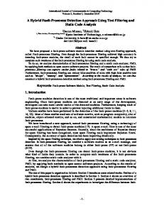
3 Residual generation with H− , H∞ and H− /H∞ optimizations Singular values [dB]

10

0

gain to worst case disturbance

−10

−20 −1 10

0

1

2

10 10 Frequency [rad/sec]

10

Figure 3.1: The singular value plot for the example system Example 3.1. Consider a stable linear system described by x˙ = Ax + Ed d y = Cx + Fd d with

⎛ ⎜ A=⎜ ⎜ ⎝

C =(

(3.1)

−6 −8 0 0 ⎞ ⎛ 1 0 0 0 ⎟ ⎜ ⎟,E = ⎜ 0 0 −6 −4 ⎟ d ⎜ ⎝ 0 0 2 0 ⎠

2 0 0 0

0 0 2 0

⎞ ⎟ ⎟ ⎟ ⎠

1 0 2.5 1 0 0.25 ) ) , Fd = ( 0 0 0 0.5 2.5 1.25

The related transfer function is Gd (s) = C(sI−A)−1 Ed +Fd . The L2 gain from disturbance d to the signal y changes with the direction and frequency of the disturbance vector. Figure 3.1 shows the plot of principal gains (gain to two extreme cases of disturbance vector directions) for the system. It can be seen that for the disturbance vector in certain direction and of specific frequency, the gain ∥y∥2 /∥d∥2 is the maximum, this specific disturbance is called the worst case disturbance (because it has the maximum effects on y) and the corresponding gain is referred to as the H∞ norm, i.e. ∥Gd ∥∞ = sup σ ¯ (Gd (jω)) = sup ω

d≠0

∥y∥2 ∥d∥2

where σ ¯ (Gd (jω)) represents the upper principal gain of Gd (jω) and ∥⋅∥2 represents the L2 norm of a signal. It is clear that if the fault detection filter is so designed to achieve a specific level of attenuation α to the worst case disturbance, surely any disturbance will have attenuation greater than or equal to α. The concept of worst case disturbance and hence H∞ disturbance attenuation can be generalized to nonlinear systems. Consider a nonlinear system described by ⎧ ⎪ ⎪x˙ = a(x) + Ed (x)d ΣD ∶ ⎨ ⎪ ⎪ ⎩y = c(x) + Fd (x)d

32

(3.2)

Singular values [dB]

10

0

−10 gain to worts case fault

−20 −1 10

0

1

2


10

Figure 3.2: The singular value plot for the example system then the H∞ norm for the nonlinear system ΣD is given as ∥ΣD ∥∞ = sup d≠0

∥y∥2 ∥d∥2

To explain the concept of H− fault sensitivity, we examine an example of a linear system. Example 3.2. Consider a linear system described by x˙ = Ax + Ef f y = Cx + Ff f ⎛ ⎜ A=⎜ ⎜ ⎝

C =(

(3.3)

−9 −4 0 0 ⎞ ⎛ 2 2 0 0 0 ⎟ ⎜ 0 ⎟ , Ef = ⎜ ⎜ 0 0 0 −9 −4 ⎟ ⎠ ⎝ 0 0 0 2 0

0 0 4 0

⎞ ⎟ ⎟ ⎟ ⎠

1 0 −2 −0.5 0 0.125 ) ) , Ff = ( 0 2 0 0.25 −4 −1.5

The related transfer function is Gf (s) = C(sI − A)−1 Ef + Ff . The L2 gain from fault f to the signal y changes with the direction and frequency of the fault vector. Figure 3.2 shows the plot of principal gains for the system. It can be seen that for the fault vector in certain direction and specific frequency, the gain ∥y∥2 /∥f ∥2 is the minimum, this specific fault is called the worst case fault (because it has the minimum effects on y and is, therefore difficult to be detected as compared to a fault of same magnitude with different direction) and the corresponding gain is referred to as the H− index, i.e. ∥y∥2 f ≠0 ∥f ∥ 2

∥Gf ∥− = inf σ(Gf (jω)) = inf ω

where σ(Gf (jω)) represents the lower principal gain of Gf (jω).

It is obvious that if the worst fault has an L2 gain ∥y∥2 / ∥f ∥2 greater than or equal to a given positive constant β, then all the faults will have gain greater than or equal to β. The

33

3 Residual generation with H− , H∞ and H− /H∞ optimizations concept of H− can be generalized to nonlinear systems. For a nonlinear system described by ⎧ ⎪ ⎪x˙ = a(x) + Ef (x)f (3.4) ΣF ∶ ⎨ ⎪ y = c(x) + F ⎪ f (x)f ⎩ H− index for the system ΣF can be defined as ∥y∥2 f ≠0 ∥f ∥ 2

∥ΣF ∥− = inf

For a more practical application, it is useful to define H∞ norm and H− index over a finite horizon [0, t1 ] as described in the following definitions. Definition 3.1. Given nonlinear system (3.2), the H∞ norm of the system ΣD in finite horizon case represented by ∥ΣD ∥∞,[0,t1 ] is defined as √ t where ∥y∥2,[0,t1 ] = ∫0 1 y T ydt

∥ΣD ∥∞,[0,t1 ] = sup d≠0

∥y∥2,[0,t1 ] ∥d∥2,[0,t1 ]

Definition 3.2. Given nonlinear system (3.4), the H− index of the system ΣF in finite horizon case represented by ∥ΣF ∥−,[0,t1 ] is defined as ∥ΣF ∥−,[0,t1 ] = inf

f ≠0

∥y∥2,[0,t1 ]

∥f ∥2,[0,t1 ]

H− fault sensitive filter design has received considerable interests for linear systems [53–55]. As far as nonlinear systems are concerned, H− fault sensitivity problem has not been addressed. The H− fault sensitive FDF design problem for nonlinear systems will be formulated in Section 3.1 and a solution will be presented in Section 3.2. There has been an extensive research to design H∞ disturbance attenuation filter, both for linear [50, 128–131] as well as nonlinear systems [114, 117, 120, 132]. However, that research is mainly focused on state estimation rather than output estimation. In Section 3.3, the difference between the two estimation problems will be highlighted. For the purpose of fault detection, output estimation is of importance and state estimation is of little use. To our knowledge, the H∞ disturbance attenuation problem for fault detection in nonlinear systems has not been studied. The problem of H∞ disturbance attenuation FDF will be formulated in Section 3.1 and a solution to this problem will be presented in Section 3.3. The H∞ based fault detection filter attenuates the effects of disturbances on the residual signal, but at the same time, may also result in the attenuation of the effects of faults on the residual signal, which is not desired. Similarly, the H− index based fault detection filter makes the residual more sensitive to faults, but at the same time may also result in amplification of the effect of disturbances on the residual signal, this is also not desired. To attain simultaneous H− fault sensitivity and H∞ disturbance attenuation, the multiobjective H− /H∞ index was proposed in [56]. The multi-objective H− /H∞ index based fault detection filter for linear systems has been widely studied and LMI solutions are presented [13, 55]. This problem for nonlinear systems is formulated in Section 3.1 and the solution is provided in Section 3.4.

34

3.1 Problem formulation

3.1 Problem formulation Consider the affine nonlinear systems described by ⎧ ⎪ ⎪x˙ = a(x) + Ed (x)d + Ef (x)f ⎨ ⎪ ⎪ ⎩y = c(x) + Fd (x)d + Ff (x)f

(3.5)

where x ∈ Rn is the state vector, y ∈ Rm is the measurement vector, d ∈ Rkd is the vector of unknown inputs (which include disturbances and measurement noise) and f ∈ Rkf is the fault vector to be detected, the time argument of these vectors is omitted for notational simplicity. All the elements in the vectors a(x) ∈ Rn , c(x) ∈ Rm and the matrices Ef (x) ∈ Rn×kf , Ed (x) ∈ Rn×kd , Ff (x) ∈ Rm×kf , Fd (x) ∈ Rm×kd are smooth functions of their arguments. For the purpose of fault detection, we apply the following nonlinear FDF ⎧ xˆ˙ = a(ˆ x) + L(ˆ x, t)(y − yˆ) ⎪ ⎪ ⎪ ⎪ ⎨yˆ = c(ˆ x) ⎪ ⎪ ⎪ ⎪ ⎩r = y − yˆ

(3.6)

where xˆ ∈ Rn is the estimate of the state vector, yˆ ∈ Rm is the estimate of the measurement vector, L(ˆ x, t) ∈ Rn×m is the filter gain matrix and r ∈ Rm is residual vector which is used to decide about the occurrence of faults. Combining the the system state vector and the filter state vector, the dynamics of the residual generator become ⎧ ⎪ ˜(˜ x) + E˜d (˜ x)d + E˜f (˜ x)f ⎪x˜˙ = a (3.7) ΣA ∶ ⎨ ⎪ r = c ˜ (˜ x ) + F ⎪ d (x)d + Ff (x)f ⎩ where x˜ = [

E˜f (˜ x) = [

a(x) x ] ],a ˜(˜ x) = [ a(ˆ x) + L(ˆ x, t)˜ c(˜ x) xˆ

Ed (x) Ef (x) ] , c˜(˜ x) = c(x) − c(ˆ x) ] , E˜d (˜ x) = [ L(ˆ x, t)Fd (x) L(ˆ x, t)Ff (x)

To achieve the sensitivity and robustness features of the fault detection filter, the following three filtering problems are formulated. Problem 3.1. H− fault detection filter design Given system (3.7) and a constant β > 0, find a filter gain matrix L(ˆ x, t) such that the L2 gain from fault to the residual is greater than or equal to β, i.e., ∥ΣA ∥−,[0,t1 ] = inf

d=0,f ≠0

∥r∥2,[0,t1 ]

∥f ∥2,[0,t1 ]

≥β

(3.8)

Problem 3.2. H∞ fault detection filter design Given system (3.7) and a constant α > 0, find a filter gain matrix L(ˆ x, t) such that the L2 gain from disturbance to the residual is less than or equal to α, i.e., ∥ΣA ∥∞,[0,t1 ] = sup

f =0,d≠0

∥r∥2,[0,t1 ]

∥d∥2,[0,t1 ]

≤α

(3.9)

35

3 Residual generation with H− , H∞ and H− /H∞ optimizations Problem 3.3. H− /H∞ fault detection filter design Given system (3.7) and two scalars α > 0 and β > 0, find a filter gain matrix L(ˆ x, t) such that 1. The L2 gain from disturbance to the residual is less than or equal to α, i.e., ∥ΣA ∥∞,[0,t1 ] = sup

f =0,d≠0

∥r∥2,[0,t1 ]

∥d∥2,[0,t1 ]

≤α

(3.10)

2. The L2 gain from fault to the residual is greater than or equal β, i.e., ∥ΣA ∥−,[0,t1 ] = inf

d=0,f ≠0

∥r∥2,[0,t1 ]

∥f ∥2,[0,t1 ]

≥β

(3.11)

Remark 3.1. In the above formulation, the effect of known inputs u has not been taken into account. However, in any fault detection system, it is desired that, additional to robustness against unknown inputs, the residual signal should be robust against the known inputs as well. In linear systems, the effect of known inputs on the residual generator dynamics is canceled out, but this is not the situation in nonlinear systems. Thus we should examine the following augmented system ⎧ ˜ x)u + E˜d (˜ ⎪ ˜(˜ x) + B(˜ x)d + E˜f (˜ x)f ⎪x˜˙ = a ⎨ ˜ x)u + Fd (x)d + Ff (x)f ⎪ x) + D(˜ ⎪ ⎩r = c˜(˜ Since it is desired that the residual signal should be robust against known inputs u, we may treat them in the same way as the unknown inputs d, i.e., for the above augmented system, we may write as ⎡ ⎤ ⎧ ⎪ ⎢ u ⎥ ⎪ ⎪ ⎢ ⎥ + E˜f (˜ ˙ ˜ x) E˜d (˜ ⎪ x)f ] x ˜ = a ˜ (˜ x ) + [ B(˜ x ) ⎪ ⎢ ⎥ ⎪ ⎪ ⎢ d ⎥ ⎪ ⎣ ⎦ ⎨ (3.12) ⎡ ⎤ ⎪ ⎥ ⎢ ⎪ u ⎪ ˜ x) Fd (x) ] ⎢⎢ ⎥⎥ + Ff (x)f ⎪ r = c˜(˜ x) + [ D(˜ ⎪ ⎪ ⎪ ⎢ d ⎥ ⎪ ⎩ ⎣ ⎦ defining u ˜ x) E˜d (˜ ˜ x) Fd (x) ] x) = [ B(˜ x) = [ D(˜ w = [ ] , E˜w (˜ x) ] , Fw (˜ d

the system (3.12) is transformed into ⎧ ⎪ ˜(˜ x) + E˜w (˜ x)w + E˜f (˜ x)f ⎪x˜˙ = a (3.13) ⎨ ⎪ r = c ˜ (˜ x ) + F x )w + F ⎪ w (˜ f (x)f ⎩ which is in the same form as (3.7) and we may perform a similar analysis as will be done for (3.7).

The approach to solve the above stated filtering problems will be based on two-players zero-sum differential game theory, a brief description of two-players zero-sum differential games is presented in Appendix A. For a more detailed study, the reader is referred to [133], and to [134] for particular focus to control problems. In next section, a game-theoretic approach to provide a solution of the H− FDF design problem is presented.

36

3.2 H− fault sensitive FDF

3.2 H− fault sensitive FDF

The minimum sensitivity problem defined in Problem 3.1 is satisfied if the functional defined by t1

J (L, f ) ≜ ∫ {rT r − β 2 f T f } dt ; d = 0

(3.14)

0

is greater than or equal to zero for each possible fault. This can be viewed as a two player zero-sum differential game with the cost functional (3.14). The minimizing player tries to minimize the functional through f and the maximizing player maximizes the functional through L. Below we present a theorem which provides a solution to the sensitivity problem. Vx and Vxˆ are row vectors of first partial derivatives of V with respect to x and xˆ, respectively. Theorem 3.1. Given system (3.7), a positive constant β and assume A1. Rf ≜ FfT (x)Ff (x) − β 2 Ikf > 0 A2. Ff (x) is a square matrix If there exists a function V (˜ x, t) with V (˜ x(0), 0) = 0 that satisfies the following HamiltonJacobi-Isaacs (HJI) equation −

∂V (˜ x, t) = Vx (˜ x, t)a(x) + Vxˆ (˜ x, t)a(ˆ x) ∂t + c˜T (˜ x)(Ff (x)Rf−1 FfT (x))−1 c˜(˜ x) − c˜T (˜ x)˜ c(˜ x)

− Vx (˜ x, t)Ef (˜ x)(FfT (x)Ff (x))−1 FfT (x)˜ c(˜ x) (3.15)

then L⋆ (ˆ x, t) satisfying

Vxˆ (˜ x, t)L⋆ (ˆ x, t) = −Vx (˜ x, t)Ef (x)(FfT (x)Ff (x))−1 FfT (x)

solves the sensitivity problem (3.8).

+ 2˜ cT (˜ x)(Ff (x)Rf−1 FfT (x))−1 − 2˜ cT (˜ x) (3.16)

Proof. For the augmented system (3.7) with the cost functional (3.14), utilizing the standard concepts from dynamic game theory we conclude that, if there exists continuously differentiable function V (˜ x, t) on [0, t1 ] × Rn , satisfying the following Hamilton-JacobiIsaacs equation −

∂V (˜ x, t) ∂V (˜ x, t) ˙ = max mink { x˜ + rT r − β 2 f T f } n×m L∈R f ∈R ∂t ∂ x˜

= max mink { Vx (˜ x, t)a(x) + Vx (˜ x, t)Ef (x)f + Vxˆ (˜ x)a(ˆ x) n×m L∈R

f ∈R

+ Vxˆ (˜ x, t)L(ˆ x, t)˜ c(˜ x) + Vxˆ (˜ x, t)L(ˆ x, t)Ff (x)f +rT r − β 2 f T f }

=Vx (˜ x, t)a(x) + Vx (˜ x, t)Ef (x)f ⋆ + Vxˆ (˜ x, t)a(ˆ x) ⋆ ⋆ + Vxˆ (˜ x, t)L (ˆ x, t)˜ c(˜ x) + Vxˆ (˜ x, t)L (ˆ x, t)Ff (x)f ⋆

37

3 Residual generation with H− , H∞ and H− /H∞ optimizations + rT (f ⋆ )r(f ⋆ ) − β 2 f ⋆ T f ⋆

(3.17)

then the pair of strategies (L⋆ , f ⋆ ) provides a saddle-point solution, i.e. J (L, f ⋆ ) ≤ J (L⋆ , f ⋆ ) ≤ J (L⋆ , f ). Furthermore, saddle-point value of the game is J (L⋆ , f ⋆ ) = V (˜ x(0), 0). This ensures J (L⋆ , f ) ≥ V (˜ x(0), 0) = 0, which in turn guarantees that L⋆ solves the sensitivity problem (3.8). Henceforth, for the sake of simplicity of notation, we will not write the arguments of the functions except where it makes ambiguity. Rest of the proof consists of finding f ⋆ and L⋆ and substituting them into (3.17). For that purpose, we define the following Hamiltonian function H (L, f ) ≜Vx˜ x˜˙ + rT r − β 2 f T f =Vx a(x, t) + Vx Ef f + Vxˆ a(ˆ x, t) + Vxˆ L˜ c + Vxˆ LFf f + rT r − β 2 f T f

(3.18)

To find f ⋆ (the fault which has the minimum effect on the residual), we differentiate H with respect to f (standard results from matrix calculus are applied, Appendix B gives a table of these results, details can be found in any reference for matrix calculus). It turns out ∂H (L, f ) ∂r =Vx Ef + Vxˆ LFf + 2rT − 2β 2 f T ∂f ∂f =Vx Ef + Vxˆ LFf + 2rT Ff − 2β 2 f T =Vx Ef + Vxˆ LFf + 2˜ cT Ff + 2f T FfT Ff − 2β 2 f T

For f ⋆ to be the critical point,

⇒

∂H (L,f ) ∣ ⋆ ∂f f =f

= 0. Hence, we get an expression for f ⋆

Vx Ef + Vxˆ LFf + 2˜ cT Ff + 2f ⋆ T FfT Ff − 2β 2 f ⋆ T = 0

Vx Ef + Vxˆ LFf + 2˜ cT Ff + 2f ⋆ T (FfT Ff − β 2 Ikf ) = 0

1 f ⋆ = − Rf−1 (EfT VxT + FfT LT VxˆT + 2FfT c˜) 2 represents the identity matrix of dimensions kf × kf and Rf = (FfT Ff − β 2 Ikf ). ⇒

where Ikf

It follows from Assumption A1 that

∂ 2 H (L,f ) ∣ ⋆ ∂f 2 f =f

= (2FfT Ff −2β 2 Ikf ) > 0, which means

f ⋆ really minimizes the Hamiltonian function. Substitute f = f ⋆ in (3.18), we obtain the following expression H (L, f ⋆ ) = Vx a(x) + Vx Ef f ⋆ + Vxˆ a(ˆ x) + Vxˆ L˜ c + Vxˆ LFf f ⋆

after simplifications,

+ (˜ c + Ff f ⋆ )T (˜ c + Ff f ⋆ ) − β 2 f ⋆ T f ⋆

1 1 H (L, f ⋆ ) = Vx a(x) − Vx Ef Rf−1 EfT VxT − Vx Ef Rf−1 FfT LT VxˆT 4 4 1 −1 T − Vx Ef Rf Ff c˜ + Vxˆ a(ˆ x) + Vxˆ L˜ c − Vxˆ LFf Rf−1 EfT VxT 4 1 −1 T T T − Vxˆ LFf Rf Ff L Vxˆ − Vxˆ LFf Rf−1 FfT c˜ + c˜T c˜ − c˜T Ff Rf−1 FfT c˜ (3.19) 4

38

3.2 H− fault sensitive FDF Since all the terms in above expression are scalars, for the purpose of simplification we may replace some terms by their transpose. As a result: 1 1 H (L, f ⋆ ) = Vx a(x) − Vx Ef Rf−1 EfT VxT − Vx Ef Rf−1 FfT LT VxˆT 4 2 1 −1 T − Vx Ef Rf Ff c˜ + Vxˆ a(ˆ x) + Vxˆ L˜ c − Vxˆ LFf Rf−1 FfT LT VxˆT 4 − Vxˆ LFf Rf−1 FfT c˜ + c˜T c˜ − c˜T Ff Rf−1 FfT c˜ To find L⋆ , set

∂H (L,f ⋆ ) ∣ ⋆ ∂L L=L

= 0 to get:

1 1 VxˆT c˜T − VxˆT Vx Ef Rf−1 FfT − VxˆT Vxˆ L⋆ Ff Rf−1 FfT − VxˆT c˜T Ff Rf−1 FfT = 0 2 2 from which we obtain an expression for L⋆ Vxˆ L⋆ = −Vx Ef (FfT Ff )−1 FfT + 2˜ cT (Ff Rf−1 FfT )−1 − 2˜ cT

It remained to prove by taking the second derivative of Hamiltonian, that L⋆ maximizes the Hamiltonian. So 1 ∂ 2 H (L, f ⋆ ) ∣ = − (Ff Rf−1 FfT ⊗ VxˆT Vxˆ )T 2 ∂L 2 L=L⋆ where ⊗ represents the Kronecker product of matrices. Since Rf is positive definite by 2 (L,f ⋆ ) Assumption A1, ∂ H∂L ∣ ⋆ will be negative definite, meaning that L⋆ will be maxi2 L=L mizing as required. Furthermore, Assumptions A1 and A2 also ensure that (FfT Ff )−1 and (Ff Rf−1 FfT )−1 exist. By substituting f ⋆ and L⋆ into (3.17) and performing some simplifications: −

∂V =Vx a(x) + Vxˆ a(ˆ x) + c˜T (Ff Rf−1 FfT )−1 c˜ − c˜T c˜ − Vx Ef (FfT Ff )−1 FfT c˜ ∂t

This completes the proof. Remark 3.2. The Assumption A1 is not specific to nonlinear systems only. A similar assumption is also made for linear systems when H− index problem is formulated. Since we are only interested in nonzero H− index, this assumption ensures that it is greater than zero. Remark 3.3. It should be noted that Assumption A2 does not cause any loss of generality. In the case that Assumption A2 is not satisfied, some fictitious fault variables can be added to make Ff (x) a square matrix. Remark 3.4. If we look at the expression (3.16) very carefully, we notice that, for a general nonlinear system, it would be quite difficult to find an L which is independent of states of the system. However, if we could somehow transform the equality in (3.15) to inequality, there would be more flexibility in the selection of V (˜ x, t) and, hence, more freedom in selection of L [114]. In that case, it will become more easier to select a state independent filter gain matrix. In this regard, the next remark is useful.

39

3 Residual generation with H− , H∞ and H− /H∞ optimizations Remark 3.5. The minimum sensitivity problem (3.8) is satisfied if t1

t1

T ∫ r rdt − β ∫ f f dt ≥ 0 T

2

0

0

the above inequality is also satisfied if for a negative semidefinite Y (˜ x(t), t) with Y (˜ x(0), 0) = 0, the following inequality holds: t1

t1

T x(t1 ), t1 ) ≥ 0 ∫ r rdt − β ∫ f f dt + Y (˜ T

2

0

0

or t1

t1

t1

d x, t)dt ≥ 0 ∫ r rdt − β ∫ f f dt + ∫ dt Y (˜ T

T

2

0

0

0

which is satisfied if rT r − β 2 f T f + or −

d Y (˜ x, t) ≥ 0 dt

∂Y (˜ x, t) ∂Y (˜ x, t) ˙ ≤ x˜ + rT r − β 2 f T f ∂t ∂ x˜

(3.20)

Note that (3.20) is similar to (3.17) except the inequality sign and that Y (˜ x, t) must be negative semidefinite. On one hand (3.20) would be better because the inequality is easy to deal with ( see Remark 3.4 ), on the other hand, it provides less freedom by restricting Y (˜ x, t) to be negative semidefinite. Here a question arises, “why to use game theory if we can obtain the sufficient conditions for the fault sensitivity, as in (3.20), without applying it?” The answer to this question is that we do not know f , therefore, we have to use its worst-case value. Game theory helps to find the worst-case fault and the corresponding best case filter gain. Combining the result from Theorem 3.1 and Remark 3.5, we have the following corollary.

Corollary 3.1. Given system (3.7), a positive constant β and assume A1. Rf ≜ FfT (x)Ff (x) − β 2 Ikf > 0 A2. Ff (x) is a square matrix If there exists a negative semidefinite function V (˜ x, t) with V (˜ x(0), 0) = 0 that satisfies the following HJI inequality −

∂V (˜ x, t) ≤ Vx (˜ x, t)a(x) + Vxˆ (˜ x, t)a(ˆ x) + c˜T (˜ x)(Ff (x)Rf−1 FfT (x))−1 c˜(˜ x) ∂t − c˜T (˜ x)˜ c(˜ x) − Vx (˜ x, t)Ef (˜ x)(FfT (x)Ff (x))−1 FfT (x)˜ c(˜ x) (3.21)


Vxˆ (˜ x, t)L⋆ (ˆ x, t) = −Vx (˜ x, t)Ef (x)(FfT (x)Ff (x))−1 FfT (x)

solves the sensitivity problem (3.8).

40


3.2 H− fault sensitive FDF Proof. The proof follows directly from Theorem 3.1 and Remark 3.5. In the case of infinite-horizon filtering problem, i.e., when t1 → ∞, and if we are interested in time-invariant gain for the filter, the function V can be selected independent of time. In that case, we can summarize the results in the following corollary. Corollary 3.2. Given system (3.7), a positive constant β and assume A1. Rf ≜ FfT (x)Ff (x) − β 2 Ikf > 0 A2. Ff (x) is a square matrix If there exists a negative semidefinite function V (˜ x) with V (˜ x(0)) = 0 that satisfies the following HJI inequality x) 0 ≤ Vx (˜ x)a(x) + Vxˆ (˜ x)a(ˆ x) + c˜T (˜ x)(Ff (x)Rf−1 FfT (x))−1 c˜(˜ then L⋆ (ˆ x) satisfying

c(˜ x) (3.23) − c˜T (˜ x)˜ c(˜ x) − Vx (˜ x)Ef (˜ x)(FfT (x)Ff (x))−1 FfT (x)˜

Vxˆ (˜ x)L⋆ (ˆ x) = −Vx (˜ x)Ef (x)(FfT (x)Ff (x))−1 FfT (x)


solves the sensitivity problem (3.8) in infinite horizon sense.

Proof. The proof follows from Corollary 3.1 by substituting a time invariant function V (˜ x).

Note that the H− fault sensitivity conditions derived above do not guarantee the stability of the filter. This is different from the H∞ disturbance attenuation problem, as will be discussed in the next section, where the disturbance attenuation condition also pledges the stability of the filter. Therefore, in designing the H− fault sensitive filter, the stability issue should be separately addressed. This can be done by selecting a positive definite Lyapunov function and showing the negative definiteness of its time derivative along the augmented system trajectories. Another common approach is to design using multi-objective H− /H∞ optimization, as will be described in Section 3.4. In this situation, the H− index gives the required level of fault sensitivity, and the stability is guaranteed by the H∞ optimization. Remark 3.6. Our solution to H− fault detection filter design involves solving an HJI inequality. We come across such HJI inequalities (equations) mostly in dealing with nonlinear systems. The analytical solution of such (inequalities) equations is, in general, hard to obtain and some numerical approach should be utilized. In case of linear systems, i.e. x˙ = Ax + Ef f + Ed d y = Cx + Ff f + Fd d

(3.25)

xˆ˙ = Aˆ x + L(ˆ x)(y − yˆ) yˆ = C xˆ

(3.26)

with a linear fault detection filter

41

3 Residual generation with H− , H∞ and H− /H∞ optimizations The simplest negative definite function to choose is V (˜ x) = (x − xˆ)T P (x − xˆ) with P ≤ 0. In this case Vx (˜ x) = 2(x − xˆ)T P = −Vxˆ (˜ x) and (3.23) is simplified as:

2(x − xˆ)T P Ax − 2(x − xˆ)T P Aˆ x + (x − xˆ)C T (Ff Rf−1 FfT )−1 C(x − xˆ)

− (x − xˆ)C T C(x − xˆ) − 2(x − xˆ)T P Ef (FfT Ff )−1 Ff C(x − xˆ) ≥ 0

(x − xˆ)T P A(x − xˆ) + (x − xˆ)T AT P (x − xˆ) + (x − xˆ)C T (Ff Rf−1 FfT )−1 C(x − xˆ)

− (x − xˆ)C T C(x − xˆ) − 2(x − xˆ)T P Ef (FfT Ff )−1 Ff C(x − xˆ) ≥ 0

P A + AT P + C T (Ff Rf−1 FfT )−1 C − C T C − 2P Ef (FfT Ff )−1 Ff C ≥ 0

(3.27)

and (3.24) simplifies to

− 2(x − xˆ)T P L⋆ = −2(x − xˆ)T P Ef (FfT Ff )−1 FfT

+ 2(x − xˆ)T C T (Ff Rf−1 FfT )−1 − 2(x − xˆ)T C T

P L⋆ = P Ef (FfT Ff )−1 FfT − C T (Ff Rf−1 FfT )−1 + C T

(3.28)

The design of H− fault sensitive FDF is an iterative procedure. One can begin with the highest possible value of β permitted by assumption A1, and check for possible existence of sufficient conditions (3.21),(3.22) ( (3.23), (3.24) for infinite horizon case). If these are not satisfied then reduce β until the sufficient conditions are fulfilled. For linear systems, these sufficient conditions are usually formulated into LMIs and the iterations are performed with efficient algorithms in MATLAB R LMI toolbox.

3.3 H∞ disturbance attenuating FDF

The H∞ nonlinear filtering has been extensively studied in literature, some references are mentioned at the beginning of this chapter. It should be explicated here that there is a delicate difference in the H∞ filtering problem and the H∞ FDF. In the former situation, the objective is to minimize ∥c(x) − c(ˆ x)∥2 ∥d∥2

(3.29)

∥c(x) − c(ˆ x) + Fd (x)d∥2 ∥y − c(ˆ x)∥2 = sup ∥d∥2 ∥d∥2 d≠0

(3.30)

sup d≠0

while in the later case, it is desired to minimize sup d≠0

For fault detection purpose, the later optimization is of more interests. To demonstrate the difference between the two optimization problems and to illustrate that satisfying (3.29) does not imply that (3.30) is also fulfilled, we give an example from linear systems.

42

3.3 H∞ disturbance attenuating FDF Example 3.3. Consider a linear system described by x˙ = Ax + Ed d y = Cx + Fd d with

A=[

0 1 ] , Ed = Fd = C = I2 −1 −1

we apply the following filter for the above system xˆ˙ = Aˆ x + L(y − yˆ) yˆ = C xˆ the error dynamics are e˙ = (A − LC)e + (Ed − LFd )d z = Ce r = Ce + Fd d

(3.31) (3.32) (3.33)

The disturbance attenuation filtering problem (3.29) is satisfied if an L satisfies the following inequality for a positive definite P P (A − LC) + (A − LC)T P +

1 P (E − LF )(E − LF )T P + C T C ≤ 0 α2

Note that the above inequality is satisfied for α = 1 and L=[

1.1454 0 1.2011 0 ] ], P = [ 0 1.1454 0 0.5344

Figure 3.3 shows the singular value plot of the system defined by (3.31) and (3.32). It ∥z∥ ¯ (w) is less than can be seen, as guaranteed by H∞ filtering problem, that supd ∥d∥2 = supw σ 2 the predefined value of α. However, as illustrated by Figure 3.4 which shows the singular ∥r∥ value plot for the system (3.31) and (3.33), the same is not guaranteed for supd ∥d∥2 . This 2 demonstrates the difference between the two filtering problems. The above example demonstrates that there is a difference between the H∞ filtering problems and H∞ fault detection filtering problems. The former have been extensively studied and some references were provided in the introduction of this chapter, while to our knowledge, the later case have not been discussed for nonlinear systems. This section is dedicated to the study of H∞ fault detection filtering problem. Similar to the H− fault sensitivity problem, we can also formulate the H∞ disturbance attenuation problem as a two-players zero-sum differential game with disturbance d and filter gain L as two players. Thus defining the cost functional t1

J (L, d) ≜ ∫ (rT r − α2 dT d)dt (f = 0)

(3.34)

0

43

3 Residual generation with H− , H∞ and H− /H∞ optimizations


−10

−20

−30 −1 10

0

1


2

10


Figure 3.3: Singular value plot for the system defined by (3.31) and (3.32)

2

0

−1.5 −1 10

0

1


2

10

Figure 3.4: Singular value plot for the system defined by (3.31) and (3.33)

44

3.3 H∞ disturbance attenuating FDF the disturbance attenuation problem (3.10) is satisfied if inf sup J (L, d) ≤ 0 L

d≠0

The following theorem gives a solution to the disturbance attenuation problem using the results from game theory. Theorem 3.2. Given system (3.7), a positive constant α and assume A1. Rd ≜ FdT (x)Fd (x) − α2 Ikd < 0 A2. Fd (x) is a square matrix If there exists a function Y (˜ x, t) with Y (˜ x(0), 0) = 0 that satisfies the following HJI equation −

∂Y (˜ x, t) = Yx (˜ x, t)a(x) + Yxˆ (˜ x, t)a(ˆ x) ∂t + c˜T (˜ x)(Fd (x)Rd−1 FdT (x))−1 c˜(˜ x) − c˜T (˜ x)˜ c(˜ x) T c(˜ x) (3.35) − Yx (˜ x, t)Ed (˜ x)(Fd (x)Fd (x))−1 FdT (x)˜


Yxˆ (˜ x, t)L⋆ (ˆ x, t) = −Yx (˜ x, t)Ed (x)(FdT (x)Fd (x))−1 FdT (x) + 2˜ cT (˜ x)(Fd (x)Rd−1 FdT (x))−1 − 2˜ cT (˜ x) (3.36)

solves the disturbance attenuation problem (3.10).

Proof. (sketch: details which are similar to the proof of Theorem 3.1 are omitted) For the system (3.7) with no fault and the cost functional (3.34), if there exists a function Y (˜ x, t) n on [0, t1 ] × R satisfying the following HJI equation −

∂Y (˜ x, t) ∂Y (˜ x, t) ˙ { = min max x˜ + rT r − α2 dT d} n×m k L∈R ∂t ∂ x˜ d∈R d

{ Yx (˜ x, t)a(x) + Yx (˜ x, t)Ed (x)d + Yxˆ (˜ x)a(ˆ x) = min max n×m k L∈R

d∈R

d

+ Yxˆ (˜ x, t)L(ˆ x, t)˜ c(˜ x) + Yxˆ (˜ x, t)L(ˆ x, t)Fd (x)d +rT r − α2 dT d }

=Yx (˜ x, t)a(x) + Yx (˜ x, t)Ed (x)d⋆ + Yxˆ (˜ x, t)a(ˆ x) ⋆ ⋆ + Yxˆ (˜ x, t)L (ˆ x, t)˜ c(˜ x) + Yxˆ (˜ x, t)L (ˆ x, t)Fd (x)d⋆

+ rT (d⋆ )r(d⋆ ) − α2 d⋆ T d⋆

(3.37)

then the pair of strategies (L⋆ , d⋆ ) provides a saddle-point solution, i.e. J (L⋆ , d) ≤ J (L⋆ , d⋆ ) ≤ J (L, d⋆ ). Furthermore, saddle-point value of the game is J (L⋆ , d⋆ ) = Y (˜ x(0), 0). This ensures J (L⋆ , d) ≤ V (˜ x(0), 0) = 0, which in turn guarantees that L⋆ solves the disturbance attenuation problem (3.10). Rest of the proof consists of finding d⋆ and L⋆ and substituting them into (3.37). For that purpose, we define the following Hamiltonian function H (L, f ) ≜Vx˜ x˜˙ + rT r − α2 dT d =Vx a(x) + Vx Ed d + Vxˆ a(ˆ x) + Vxˆ L˜ c + Vxˆ LFd d + rT r − α2 dT d

(3.38)

45

3 Residual generation with H− , H∞ and H− /H∞ optimizations Similar to the case of fault sensitivity problem, differentiate the Hamiltonian with respect to d, set the derivative equal to zero to find the worst case disturbance d⋆ = Rd−1 (EdT YxT + FdT LT YxˆT + 2FdT c˜)

Substitute the worst case disturbance in the defined Hamiltonian, differentiate it with respect to L and set the derivative equal to zero to obtain an expression for L⋆ as given in (3.36). By similar arguments as in the proof of fault sensitivity condition, it can be shown that d⋆ maximizes the Hamiltonian and L⋆ minimizes the Hamiltonian, as required. Substitute d⋆ and L⋆ in (3.37) to get (3.35). As it has been discussed, an inequality version of HJI in (3.35) would be easier to solve, therefore, it is desired to convert it into HJI inequality. This can be done by using similar arguments as used in H− sensitivity condition. These arguments are analogous to the dissipativity approach and can be stated as under: The system (3.7) is said to be dissipative with respect to supply rate of α2 ∥d∥2 + ∥r∥2

(3.39)

∂Y + Yx˜ x˜˙ − α2 dT d + rT r ≤ 0 ∂t

(3.40)

2

2

if there exists a positive function Y (˜ x, t) that satisfies

and from the definition of dissipativity, it follows that ∥r∥2 ≤ α2 ∥d∥2 2

2

Furthermore, we known that if a system is dissipative with respect to supply rate given in (3.39), then it is finite gain L2 stable [135, 136]. Thus, we can summarize the results in the form of following corollary. Corollary 3.3. Given system (3.7) with f = 0, a positive constant α and assume A1. Rd ≜ FdT (x)Fd (x) − α2 Ikd < 0 A2. Fd (x) is a square matrix If there exists a positive definite function Y (˜ x, t) with Y (˜ x(0), 0) = 0 that satisfies the following HJI inequality −

∂Y (˜ x, t) ≥ Yx (˜ x, t)a(x) + Yxˆ (˜ x, t)a(ˆ x) + c˜T (˜ x)(Fd (x)Rd−1 FdT (x))−1 c˜(˜ x) ∂t − c˜T (˜ x)˜ c(˜ x) − Yx (˜ x, t)Ed (˜ x)(FdT (x)Fd (x))−1 FdT (x)˜ c(˜ x) (3.41)

and L⋆ (ˆ x, t) satisfying

Yxˆ (˜ x, t)L⋆ (ˆ x, t) = −Yx (˜ x, t)Ed (x)(FdT (x)Fd (x))−1 FdT (x) + 2˜ cT (˜ x)(Fd (x)Rd−1 FdT (x))−1 − 2˜ cT (˜ x) (3.42)

then the system (3.7) is dissipative with respect to supply rate of (3.39) and, therefore, solves the disturbance attenuation problem (3.10).

46

3.3 H∞ disturbance attenuating FDF Note that with the dissipativity theory, we have obtained an inequality version of equation (3.35) which is easier to solve (see Remark 3.4). Furthermore, the dissipativity property also guarantees the stability of the filter. Now question arises why do we use the game theory? The answer is that with the game theoretic approach, the worst case disturbance and the corresponding optimal filter gain can be found. In the case when t1 → ∞, and we are interested in time invariant solutions, we can take a time independent function Y (˜ x). In this situation, we have the following results.

Corollary 3.4. Given system (3.7) with f = 0, a positive constant α and assume A1. Rd ≜ FdT (x)Fd (x) − α2 Ikd < 0 A2. Fd (x) is a square matrix If there exists a positive definite function Y (˜ x) with Y (˜ x(0)) = 0 that satisfies the following HJI inequality

0 ≥ Yx (˜ x)a(x) + Yxˆ (˜ x)a(ˆ x) + c˜T (˜ x)(Fd (x)Rd−1 FdT (x))−1 c˜(˜ x) − c˜T (˜ x)˜ c(˜ x) c(˜ x) (3.43) − Yx (˜ x)Ed (˜ x)(FdT (x)Fd (x))−1 FdT (x)˜

and L⋆ (ˆ x) satisfying

Yxˆ (˜ x)L⋆ (ˆ x) = −Yx (˜ x)Ed (x)(FdT (x)Fd (x))−1 FdT (x) + 2˜ cT (˜ x)(Fd (x)Rd−1 FdT (x))−1 − 2˜ cT (˜ x) (3.44)

then the systems (3.7) is dissipative with respect to supply rate of (3.39) and, therefore, solves the disturbance attenuation problem (3.10) in infinite horizon sense. Proof. The proof follows by substituting a time independent function Y (˜ x) in the results of Corollary 3.3. For the case of linear systems defined in (3.25) and the corresponding linear fault detection filter (3.26), we can select Y (˜ x) = (x − xˆ)T Q(x − xˆ) with Q ≥ 0. In this case (3.43) and (3.44) are simplified to QA + AT Q + C T (Fd Rd−1 FdT )−1 C − C T C − 2QEd (FdT Fd )−1 Fd C ≤ 0 QL⋆ (ˆ x) = QEd (FdT Fd )−1 FdT − C T (Fd Rd−1 FdT )−1 + C T

(3.45) (3.46)

Similar to the case of H− fault sensitive FDF, the H∞ disturbance attenuation FDF design is also an iterative procedure. Starting with the smallest possible value of α permitted by A1, one can successively increase α until (3.41),(3.42) are satisfied ((3.43), (3.44) in infinite horizon case are satisfied). As compared to H− fault sensitive FDF which guarantees a required level of sensitivity of residual to the faults, the H∞ disturbance attenuating FDF ensures that residual is robust against disturbances. In addition to the disturbance attenuation property, H∞ disturbance attenuating FDF also helps to set up the threshold. Thus, if L2 norm of residual signal is used as evaluation function, the maximum possible effect of disturbances on the evaluated residual is not greater than αδd , where ∥d∥2 ≤ δd . One can set threshold equal to αδd to avoid any possible false alarms. Further discussions on residual evaluation and threshold settings will be provided in Chapters 4 and 5.

47

3 Residual generation with H− , H∞ and H− /H∞ optimizations

3.4 H−/H∞ multi-objective FDF

In the last two sections, two fault detection filtering problems were discussed. In the first case, H− fault detection filter was presented which guaranteed a fault sensitivity greater than a given constant. However, this filter does not give any indication of the disturbance attenuation property of the filter. It is possible that, in addition to making residual sensitive to faults, the filter also makes residual sensitive to disturbances. This is certainly not a desired feature of H− filter. Similar is the situation for the second FDF, the H∞ fault detection filter guarantees the disturbance attenuation greater than a given constant but does not give any indication of fault sensitivity. In addition to disturbance attenuation, the filter may also result in attenuating the effect of faults. A better fault detection filter should be simultaneously robust against disturbance and sensitive to faults. For that purpose, multi-objective H− /H∞ index can be used. The multi-objective index was first proposed in [56] and later several techniques were proposed for linear systems. This section presents H− /H∞ filtering problem for nonlinear systems. In H− /H∞ based design, the objective is to maximize the ratio β/α, rather than individually maximizing β or minimizing α. Thus an H− /H∞ based filter may not be the optimal in the sense of H− index, i.e., another filter gain may exist which gives a higher fault to residual gain than that delivered by the H− /H∞ based designed filter gain. A similar comparison of H∞ based FDF and multi-objective index based FDF can be presented, i.e., the disturbance to residual gain for the former FDF may be smaller than that for the later FDF. The H− /H∞ multi-objective FDF problem can be formulated as two two-players nonzerosum differential games with following two cost functionals: t1

J1 (L, f ) = ∫ (rT r − βf T f ) dt ; d = 0

(3.47)

0

t1

J2 (L, d) = ∫ (rT r − αdT d) dt ; f = 0

(3.48)

0

The first functional is associated with H− fault sensitivity and the second cost functional is associated with the H∞ disturbance attenuation. Making J1 ≥ 0 guarantees ∥ΣA ∥−,[0,t1 ] =

inf f ≠0 ∥f ∥2,[0,t1 ] ≥ β and making J2 ≤ 0 guarantees ∥ΣA ∥∞,[0,t1 ] = supd≠0 ∥d∥2,[0,t1 ] ≤ α. The 2,[0,t1 ] 2,[0,t1 ] following theorem now gives the sufficient conditions for the solvability of the problem. ∥r∥

∥r∥

Theorem 3.3. Consider the nonlinear system (3.7), positive constants α and β and assume A1. Rf ≜ FfT (x)Ff (x) − β 2 Ikf > 0 A2. Rd ≜ FdT (x)Fd (x) − α2 Ikd < 0 A2. Ff (x), Fd (x) are square matrices Suppose that there exists a pair of functions V (˜ x, t) with V (˜ x(0), 0) = 0 and Y (˜ x, t) with V (˜ x(0), 0) = 0 and the filter gain L(ˆ x, t) satisfying the following partial differential equa48

3.4 H− /H∞ multi-objective FDF tions, 1 1 Vx a(x) − Vx Ef Rf−1 EfT VxT − Vx Ef Rf−1 FfT LT VxˆT 4 2

1 − Vx Ef Rf−1 FfT c˜ + Vxˆ a(ˆ x) + Vxˆ L˜ c − Vxˆ LFf Rf−1 FfT LT VxˆT 4

− Vxˆ LFf Rf−1 FfT c˜ + c˜T c˜ − c˜T Ff Rf−1 FfT c˜ = −

∂V ∂t

(3.49)

∂Y ∂t

(3.50)

1 1 Yx a(x) − Yx Ed Rd−1 EdT YxT − Yx Ed Rd−1 FdT LT YxˆT 4 2

1 − Yx Ed Rd−1 FdT c˜ + Yxˆ a(ˆ x) + Yxˆ L˜ c − Yxˆ LFd Rd−1 FdT LT YxˆT 4

− Yxˆ LFd Rd−1 FdT c˜ + c˜T c˜ − c˜T Fd Rd−1 FdT c˜ = −

then L(ˆ x, t) solves the multi-objective filtering problem defined in Problem 3.3. Proof. (sketch: details which are similar to the proof of Theorems 3.1, 3.2 are omitted) The proof follows by defining Hamiltonian functions H1 and H2 as in (3.18) and (3.38), respectively. Find f ⋆ and d⋆ by setting ∂H1 ∣ = 0, ∂f f ⋆

∂H2 ∣ =0 ∂d d⋆

and substitute in the Hamiltonians H1 and H2 to reach at the results. Then L which simultaneously satisfies (3.49) and (3.49) will satisfy both the sensitivity and robustness conditions. In previous sections, we derived sufficient conditions for H− fault sensitivity and H∞ disturbance attenuation fault detection filtering problems. These conditions were in form of an HJI and and explicit expression for the filter gain L. However, in H− /H∞ based multi-objective filtering problems, we can not derive an explicit expression for L, because the same L has to satisfy both the sensitivity and robustness conditions. That is, if we derive an explicit expression for L based on (3.49), it may not satisfy (3.50), and vice versa. It should be noted that the H∞ disturbance robustness condition also ensures the finite gain L2 stability of the filter (see [135, 136] for finite-gain L2 stability). Although the H− /H∞ optimization based FDF is better in the sense that it provides simultaneous disturbance attenuation and fault sensitivity, but the disadvantage is that it involves solving two coupled partial differential equations. It can be shown (as in Section 3.2 and Section 3.3) that for negative semidefinite V and positive semidefinite Y , the ‘=’ in (3.49) and (3.49) can be respectively changed to ≥ and ≤. In the case when t1 → ∞, and we are interested in time invariant filter gain L(ˆ x), the functions V and Y can be taken independent of time. Hence we have the following corollary Corollary 3.5. Consider the nonlinear system (3.7), positive constants α and β and assume A1. Rf ≜ FfT (x)Ff (x) − β 2 Ikf > 0 49

3 Residual generation with H− , H∞ and H− /H∞ optimizations A2. Rd ≜ FdT (x)Fd (x) − α2 Ikd < 0 A2. Ff (x), Fd (x) are square matrices Suppose that there exists a pair of negative definite function V (˜ x) with V (˜ x(0)) = 0 and a positive definite function Y (˜ x) with Y (˜ x(0)) = 0 and the filter gain L(ˆ x) satisfying the following partial differential equations, 1 1 Vx a(x) − Vx Ef Rf−1 EfT VxT − Vx Ef Rf−1 FfT LT VxˆT 4 2 1 −1 T ˜ − Vx Ef Rf Ff C + Vxˆ a(ˆ x) + Vxˆ L˜ c − Vxˆ LFf Rf−1 FfT LT VxˆT 4 − Vxˆ LFf Rf−1 FfT c˜ + c˜T c˜ − c˜T Ff Rf−1 FfT c˜ ≥ 0 (3.51) 1 1 Yx a(x) − Yx Ed Rd−1 EdT YxT − Yx Ed Rd−1 FdT LT YxˆT 4 2

1 x) + Yxˆ L˜ c − Yxˆ LFd Rd−1 FdT LT YxˆT − Yx Ed Rd−1 FdT c˜ + Yxˆ a(ˆ 4 − Yxˆ LFd Rd−1 FdT c˜ + c˜T c˜ − c˜T Fd Rd−1 FdT c˜ ≤ 0 (3.52)

then L(ˆ x) solves the multi-objective filtering problem defined in Problem 3.3 in infinite horizon sense. Proof. The proof follows by substituting time invariant functions V (˜ x) and Y (˜ x) in the results of Theorem 3.3.

For linear system defined in (3.25) and corresponding fault detection filter (3.26), the negative semidefinite function V (˜ x) can be selected as V (˜ x) = (x − xˆ)T P (x − xˆ) with P ≤ 0 and the positive definite function Y (˜ x) = (x − xˆ)T Q(x − xˆ) with Q ≥ 0. In this case (3.51) is simplified as under: (x − xˆ)T P A(x − xˆ) + (x − xˆ)T AT P (x − xˆ) − (x − xˆ)T P Ef Rf−1 EfT P (x − xˆ)

+ (x − xˆ)T P Ef Rf−1 FfT LT P (x − xˆ) − (x − xˆ)T P Ef Rf−1 FfT C(x − xˆ) − 2(x − xˆ)T P LC(x − xˆ) + (x − xˆ)T P LFf Rf−1 EfT P (x − xˆ)

− (x − xˆ)T P LFf Rf−1 FfT LT P (x − xˆ) + (x − xˆ)T P LFf Rf−1 FfT C(x − xˆ) + C T (x − xˆ)T C(x − xˆ) − (x − xˆ)T P Ef Rf−1 FfT C(x − xˆ)

+ (x − xˆ)T P LFf Rf−1 FfT C(x − xˆ) − C T (x − xˆ)T Ff Rf−1 FfT C(x − xˆ) ≥ 0

Since all terms in above equation are scalars which may be transposed, the above expression becomes P A + AT P − P Ef Rf−1 EfT P + P Ef Rf−1 FfT LT P − P Ef Rf−1 FfT C − P LC − C T LT P + P LFf Rf−1 EfT P − P LFf Rf−1 FfT LT P + P LFf Rf−1 FfT C

+ C T C − C T Ff Rf−1 EfT P + C T Ff Rf−1 FfT LT P − C T Ff Rf−1 FfT C ≥ 0

After a few further simplifications P (A − LC − (Ef − LFf )Rf−1 FfT C) + (A − LC − (Ef − LFf )Rf−1 FfT C)T P

− P (Ef − LFf )Rf−1 (Ef − LFf )T P + C T (Ikf − Ff Rf−1 FfT )C ≥ 0

50

3.5 An example Likewise, after similar simplifications, (3.52) is reduced to Q(A − LC − (Ed − LFd )Rd−1 FdT C) + (A − LC − (Ed − LFd )Rd−1 FdT C)T Q − Q(Ed − LFd )Rd−1 (Ed − LFd )T Q + C T (Ikd − Fd Rd−1 FdT )C ≥ 0

These are the well known result for case of linear systems (see e.g. [13, Chapter 7]). The above nonlinear matrix inequalities (NMI) can be reduced to linear matrix inequalities (LMI) and powerful tools are available to solve such LMIs.

3.5 An example To illustrate our results for nonlinear systems, we consider an example of a simple second order system. The dynamics of the system are given by x˙ 1 = x2 x˙ 2 = −bx2 − cx1 − kn sin(x2 ) + kg u + d y = x1 + f + 0.5d

(3.53)

x1 , x2 are respectively the angular position and the angular velocity of the positioning system, y is the measurement, u is the input, d is the measurement noise and f is the sensor fault to be detected. The numerical values of the system parameters are: b = 1, c = 0.4, k1 = 0.1 and kg = 1. Note that in this example, reference input u(t) is also present. Since the input matrix is independent of states, the influence of u(t) on state estimation error is removed after using an FDF. We have the following system matrices: a(x) = [

0 0 x2 ] , Ef = [ ] , Ed = [ ] , 1 0 −bx2 − cx1 − kn sin(x2 )

C = [ 1 0 ] , Ff = [ 1 ] , Fd = [ 0.5 ]

H− fault sensitive FDF It follows from Corollary 3.2 that the fault sensitivity problem (3.8) with infinite horizon case is solved for the example system if we find an L(ˆ x) and a negative definite function V (˜ x) with V (˜ x(0)) which satisfy (3.23) and (3.24). With A1 = [

equation (3.23) becomes

0 0 1 ] ] , A2 (x) = [ −kn sin(x2 ) −c −b

Vx A1 x + Vx A2 (x) + Vxˆ A1 xˆ + Vxˆ A2 (ˆ x) ˜ x) ≥ 0 (3.54) ˜ x) − C˜ T (˜ ˜ x) − Vx E(F T F )−1 F T C(˜ x)C(˜ + C˜ T (˜ x)(Ff Rf−1 FfT )−1 C(˜

We treat the stationary case (t1 → ∞) and select V = (x − xˆ)T P (x − xˆ), where P is a symmetric negative definite matrix, (3.54) becomes, (x − xˆ)T P A1 (x − xˆ) + (x − xˆ)T AT1 P (x − xˆ) + (x − xˆ)T C T (Ff Rf−1 FfT )−1 C(x − xˆ) − (x − xˆ)T C T C(x − xˆ)

− 2(x − xˆ)T P E(F T F )−1 F T C(x − xˆ) + J1 ≥ 0 (3.55) 51

3 Residual generation with H− , H∞ and H− /H∞ optimizations where J1 = 2(x − xˆ)T P A2 (x) − 2(x − xˆ)T P A2 (ˆ x) = −2kn (x − xˆ)T P [

= −2kn (x − xˆ)T P [

= −2kn (x − xˆ)T P [

= −2kn (x − xˆ)T P [ ≥ 2kn (x − xˆ)T P [

0 ] sin(x2 ) − sin(ˆ x2 )

x2 x2 +ˆ x2 ] 2 sin( x2 −ˆ 2 ) cos( 2 ) x −ˆ x x2 + xˆ2 0 sin( 2 2 2 ) ] (x2 −ˆx2 ) cos( )[ 1 2 2

0

0 1 ] (x − xˆ)

x2 + xˆ2 x2 − xˆ2 0 ) cos( ) [ 0 1 ] (x − xˆ) ] sinc( 1 2 2

0 ] [ 0 1 ] (x − xˆ) 1

x1 x1 +ˆ x1 The last inequality follows from the fact that the minimum value of sinc( x1 −ˆ 2 ) cos( 2 ) is −1 and P < 0. Hence, a sufficient condition for (3.55) becomes,

(x − xˆ)T P A1 (x − xˆ) + (x − xˆ)T AT1 P (x − xˆ) + (x − xˆ)T C T (Ff Rf−1 FfT )−1 C(x − xˆ) − 2(x − xˆ)T P Ef (FfT FF )−1 FFT C(x − xˆ) − (x − xˆ)T C T C(x − xˆ) + 2kn (x − xˆ)T P [

0 ] [ 0 1 ] (x − xˆ) ≥ 0 1

or P A1 + AT1 P + C T (Ff Rf−1 FfT )−1 C − C T C − 2P Ef (FfT Ff )−1 FfT C

+ 2kn P [

0 ][ 0 1 ] ≥ 0 1

a sufficient condition for the above inequality is P A1 + AT1 P − C T C − 2P Ef (FfT Ff )−1 FfT C + 2kn P [

0 ][ 0 1 ] ≥ 0 1

(3.56)

and the filter gain L is given by − 2(x − xˆ)T P L = −2(x − xˆ)T P Ef (FfT Ff )−1 FfT

+ 2(x − xˆ)T C T (F R−1 F T )−1 − 2(x − xˆ)T C T

or

L = Ef (FfT Ff )−1 FfT − P −1 C T (F R−1 F T )−1 + P −1 C T

The inequality (3.56) is satisfied for

P =[

52

−4.2363 −2.7369 ] −2.7369 −4.4638

(3.57)

3.5 An example

Figure 3.5: Residual signal for a unit step sensor fault which occurs at 30 s Note that F T F = 1, so according to Assumption A1, the maximum possible value of β is 1. We calculate the filter gain L for β = 0.9 to get: L=[

−0.3166 ] 0.1941

(3.58)

The example was simulated in Simulink R for a unit step fault which occurs at 30 seconds in the sensor measuring the angular position of the system. The initial conditions of the positioning system were set as [0.2 0] in simulation. The simulation results are shown in the Figure 3.5. It can be observed that the residual signal is sufficiently sensitive to the fault. Some further discussion on this figure will be made in H∞ based FDF design. H∞ disturbance attenuating FDF Now we design an H∞ disturbance attenuating FDF for the example system. It follows Corollary 3.4 that the H∞ disturbance attenuation problem with infinite horizon case is achieved if there exits a positive definite function Y (˜ x) with Y (˜ x(0)) which satisfies (3.43), the filter gain L(ˆ x) is then given by (3.44). With the matrices A1 and A2 (x) defined above, (3.43) becomes ˜ x) Yx A1 x + Yx A2 (x) + Yxˆ A1 xˆ + Yxˆ A2 (ˆ x) + C˜ T (˜ x)(Fd Rd−1 FdT )−1 C(˜ ˜ x) − Yx Ed (F T Fd )−1 F T C(˜ ˜ x) ≤ 0 (3.59) − C˜ T (˜ x)C(˜ d d

Select Y (˜ x) = (x − xˆ)T Q(x − xˆ), with Q ≥ 0, (3.59) reduces to

(x − xˆ)T QA1 (x − xˆ) + (x − xˆ)T AT1 Q(x − xˆ) + (x − xˆ)T C T (Fd Rd−1 FdT )−1 C(x − xˆ) − (x − xˆ)T CC(x − xˆ) − 2(x − xˆ)T QEd (FdT Fd )−1 FdT C(x − xˆ) + J2 ≤ 0 (3.60)

where

J2 = 2(x − xˆ)T P A2 (x) − 2(x − xˆ)T P A2 (ˆ x)

with similar simplifications as for J1 , we reach at J2 = −2kn (x − xˆ)T Q [

x2 − xˆ2 x2 + xˆ2 0 ] sinc( ) cos( ) [ 0 1 ] (x − xˆ) 1 2 2 53

3 Residual generation with H− , H∞ and H− /H∞ optimizations x2 x2 +ˆ x2 Noting that Q ≥ 0 and that sinc( x2 −ˆ 2 ) cos( 2 ) can have values in between −1 and 1, we conclude

−2kn (x − xˆ)T Q [

0 0 ] [ 0 1 ] (x − xˆ) ≤ J2 ≤ 2kn (x − xˆ)T Q [ ] [ 0 1 ] (x − xˆ) 1 1

Thus sufficient condition for (3.60) is (x − xˆ)T QA1 (x − xˆ) + (x − xˆ)T AT1 Q(x − xˆ) + (x − xˆ)T C T (Fd Rd−1 FdT )−1 C(x − xˆ) − (x − xˆ)T CC(x − xˆ) − 2(x − xˆ)T QEd (FdT Fd )−1 FdT C(x − xˆ) + 2kn (x − xˆ)T Q [

0 ] [ 0 1 ] (x − xˆ) ≤ 0 1

which simplifies to QA1 + AT1 Q + C T (Fd Rd−1 FdT )−1 C − CC

− 2QEd (FdT Fd )−1 FdT C + 2kn Q [

0 ] [ 0 1 ] ≤ 0 (3.61) 1

and the expression for L(ˆ x) is obtained from (3.44)

L = Ed (FdT Fd )−1 FdT − 2Q−1 C T (Fd Rd−1 FdT )−1 − 2Q−1 C T

(3.62)

The following positive definite Q solves (3.61) for α = 0.5 (the minimum possible value of α), Q=[

2.8407 0.8441 ] 0.8441 4.6377

and from (3.62), the filter gain L is L=[

0.3024 ] 0.9450

Figure 3.6 shows the simulation results for a unit step sensor fault which occurs at 50 seconds. It can be seen that the effect of disturbances on the residual signal is considerably reduced. The disturbance and the sensor noise is bounded by d ∈ [−0.2, 0.2]. Discussions In this example, we have designed two filters for the example system: an H− fault sensitive FDF and an H∞ disturbance attenuation FDF. The inset figures in Figure 3.5 and Figure 3.6 show that the H∞ disturbance attenuating filter has a better disturbance attenuation property. But at the same time we can notice that the H− fault sensitive filter provides better sensitivity to the faults.

54

3.6 Summary

Figure 3.6: Residual signal for a unit step sensor fault which occurs at 30 s

3.6 Summary Residual generation is an important step in observer-based fault detection of dynamic systems. The residual signal is obtained by comparing the measurements with their estimates generated by the observer (filter). For a better performance of the fault detection system, it is desired that the designed observer (filter) should have the properties such that the residual signal is sensitive to faults and robust against disturbances. To measure sensitivity to faults and robustness against disturbances, the worst case scenario is usually examined. For that purpose H− index and H∞ norm are widely used in literature. This chapter explained the basic idea of H− index and H∞ norm and their application in fault detection. To achieve fault sensitivity, H− fault sensitive FDF was presented for nonlinear systems. The H− fault sensitive FDF ensures that the L2 gain from worst case fault (the fault for which the residual is minimally sensitive) to the residual is greater than a known constant. To deal with the disturbance attenuation, H∞ disturbance attenuating FDF was proposed. The difference between extensively studied H∞ filtering problem and the H∞ fault detection filtering problem was emphasized with an example. The later is of more interest for fault detection but has not been discussed for nonlinear systems. The proposed H∞ disturbance attenuating filter guarantees that the L2 gain from worst case disturbance to the residual is less than a known constant. It was highlighted that, additional to fault sensitivity, the H− fault sensitive FDF may also result in sensitivity to disturbances. Likewise, the H∞ disturbance attenuating FDF may result in attenuation of faults additional to attenuation of disturbances. This is, off course, not desired. The simultaneous attenuation of disturbances and amplification of faults should be attained. To achieve this objective, the H− /H∞ multi-objective FDF was proposed. In all the three proposed fault detection filters, both finite horizon and infinite horizon cases were addressed. It was shown that for linear systems, our results reduce to well known results for linear systems. The proposed FDF methods were illustrated with simulation example of a simple second order system.

55

Chapter

4

Dynamic threshold computation The main contribution of this chapter includes the presentation of a method for generating dynamic threshold for a class of nonlinear systems. For systems with Lipschitz nonlinearities and unstructured uncertainties, an inequality for the upper bound on the modulus of error dynamics is derived. This upper bound is utilized for designing a dynamic threshold. The effectiveness of the proposed technique is demonstrated by simulation results of an simple Lipschitz nonlinear system. As discussed in Chapter 2, the process of model-based fault detection consists of two steps, residual generation and residual evaluation. In observer-based residual generation techniques, estimations of the measurements are generated using observers and the residual is the difference of the two. In ideal case, when there are no disturbances and modeling uncertainties, residual becomes zero in the absence of faults. A deviation from zero gives the indication of presence of fault. In reality, such ideal conditions never exist and there are always disturbances and uncertainties. This results in the residual signal being nonzero even in the absence of faults. The aim of residual evaluation is to decide whether a fault has occurred or not even in the presence of modeling uncertainties and disturbances. For that purpose, residual is evaluated and then compared to some threshold to decide about the presence of faults. Selection of threshold plays an important role in the performance of a fault detection system. If a constant threshold is used and is selected too high, it may result in mis-detection of faults, whereas if it is selected too low, some of disturbances may

Figure 4.1: Comparison of a constant and a variable thresholds for fault detection

57

4 Dynamic threshold computation

(a) Classical method for variable threshold generation: threshold is generated by multiplying the input with norm of uncertainties

(b) Dynamic threshold generation: the threshold generator is a dynamic system

Figure 4.2: Classical method for variable threshold generation vs dynamic threshold generation cause the residual to cross the threshold and result in false-alarm. To avoid this difficulty, as proposed by [137], one can use variable or adaptive threshold which varies according to the control activity and uncertainties in the plant. Figure 4.1 compares a constant threshold to a variable threshold . It can be noticed that a constant threshold either results in miss-detection of faults (if selected too high) or some of the uncertainties appear as faults (if threshold is selected too low). Whereas, the variable threshold can successfully avoid false alarms generated by uncertainties and, thus improves the fault detectability. Several techniques have been presented in the literature for designing adaptive threshold for linear systems. For example, [43] proposed frequency domain approach to design an adaptive threshold, [138] used the statistical approach to design adaptive threshold. Recently, [122], [139], [140] proposed the idea of dynamic threshold generation which not only varies according to control activity, but also possesses dynamic properties and hence, is more tighter to the fault-free residual signal resulting in better fault detection system. Figure 4.2 show the difference of a classical adaptive threshold generator and a dynamic threshold generator. In the domain of nonlinear systems, only a few articles address the problem of threshold generation[141], [126], [127]. In this chapter, a the time domain approach for dynamic threshold generation for Lipschitz nonlinear systems is proposed. The threshold generated is adaptive in nature and the on-line implementation does not involve complex mathematical computation.

4.1 Problem formulation Consider Lipschitz nonlinear systems described by x˙ = Ax + φ(x, u) + η(x, u, t) + Ef f y = Cx + Ff f

(4.1) (4.2)

where x ∈ Rn is the system state vector, u ∈ Rm is the input vector, y ∈ Rp is the measurable output vector, φ ∶ Rn × Rm ↦ Rn and η ∶ Rn × Rm × R+ ↦ Rn are smooth vector fields. Ef ,

58

4.1 Problem formulation Ff are the fault input and output matrices, respectively, and C is the output matrix of appropriate dimensions. It is assumed that the modeling uncertainty η, which may also include external disturbances, is unstructured and is an unknown nonlinear function of u and t, but it is bounded by some known functional, i.e., ∣η(x, u, t)∣ ≤ η¯(u, t)

φ(x, u) is nonlinearity with a Lipschitz constant γ, i.e., ∣φ(x, u) − φ(x − e, u)∣ ≤ γ∣e∣

As discussed in [142], the class of systems covered by (4.1) is fairly general and any nonlinear system of the form x˙ = f (x, u) can be expressed in form (4.1) as long as f (x, u) is differentiable with respect to x. In addition, most of the nonlinearities may be considered as Lipschitz at least locally. For the purpose of fault detection, we need to generate a residual signal which carries the information about faults. To generate such a residual for system (4.1)-(4.2), we take the observer of the form xˆ˙ = Aˆ x + φ(ˆ x, u) + L[y − C xˆ] yˆ = C xˆ

(4.3)

Several techniques for observer design for Lipschitz nonlinear systems exist in the literature. Some of the most commonly applied to fault detection have been described in Chapter 2. These include the Thau’s observers, high gain observers [94], [98], [95], sliding mode observers, etc. The approach developed in Chapter 3 for fault sensitive detection filter design can also be utilized. Other important observer design approaches for Lipshcitz nonlinear systems are the distance to unobservability based observer [142, 143] and observer design for systems with large Lipschitz constant [144]. Here, we assume that such an observer is already designed. The residual is simply defined as r = y − yˆ

Introducing the variable e = x − xˆ, the dynamics of residual generator can be written as x˙ = Ax + φ(x, u) + η(x, u, t) + Ef f e˙ = (A − LC)e + φ(x, u) − φ(x − e, u) + η(x, u, t) + Ef f r = Ce + Ff f

Using the simplified notation A¯ = A−LC and Φ(x, e, u) = φ(x, u)−φ(x−e, u), the dynamics of the residual generator can be written as x˙ = Ax + φ(x, u) + η(x, u, t) + Ef f ¯ + Φ(x, e, u) + η(x, u, t) + Ef f e˙ = Ae r = Ce + Ff f Due to the presence of disturbances and modeling uncertainties, the residual signal will not be zero even in the absence of faults. Residual evaluation and threshold setting serves to

59

4 Dynamic threshold computation avoid the effect of uncertainties and disturbances. A decision on the occurrence of a fault is then made by comparing the evaluated residual to the threshold. Some standard evaluation functions are described in Chapter 2. As proposed in [122], the following evaluation function is used, t

J = ∥r∥v ≜ ∫ v(t − τ ) ∣r(τ )∣ dτ = (v ∗ ∣r∣)(t) 0

Where v is the weighting function which increases the influence of the most recent data. A simple choice of v could be an exponential function µe−µt which has the advantage that the convolution with v can be implemented by a simple first order transfer function. Two major advantages of using the above evaluation function are mentioned in [122]. Firstly, the absolute value of the residual is likely to be less sensitive to outliers than the square and secondly, it provides efficient ways of calculating the robust threshold. Threshold is then selected as Jth = sup ∥r∥v

(4.4)

fault-free

and the following decision logic is used to detect the occurrence of faults: J > Jth ⇒ fault alarm J ≤ Jth ⇒ no alarm Designing an optimum threshold, which avoids false alarm with maximum probability of fault detection is the design problem. The main task is to develop a method for generating dynamic threshold for fault detection for the system (4.1) - (4.2).

4.2 Preliminaries and notations Before we are able to proceed for further discussion, it will be useful to present some preliminary material. The convolution between two functions F and G will be represented as FG, i.e., FG ≜ F ∗ G

The element-wise inequalities between matrices and vectors will be represented by t and u, for example, with ⎡ x11 ⋯ x1m ⎢ ⎢ ⋮ X ≜⎢ ⋮ ⋱ ⎢ ⎢ xn1 ⋯ xnm ⎣

⎤ ⎡ y11 ⋯ y1m ⎥ ⎢ ⎥ ⎢ ⋮ ⎥, Y ≜ ⎢ ⋮ ⋱ ⎥ ⎢ ⎥ ⎢ yn1 ⋯ ynm ⎦ ⎣

⎤ ⎥ ⎥ ⎥ ⎥ ⎥ ⎦

then X t Y means that xij ≤ yij for all i ∈ 1⋯n and all j ∈ 1⋯m. ∣ ⋅ ∣ will represent the matrix modulus function, i.e. element-wise absolute value. Thus ⎡ ∣x11 ∣ ⋯ ∣x1m ∣ ⎢ ⎢ ⋱ ⋮ ∣X∣ = ⎢ ⋮ ⎢ ⎢ ∣xn1 ∣ ⋯ ∣xnm ∣ ⎣

60

⎤ ⎥ ⎥ ⎥ ⎥ ⎥ ⎦

4.3 Dynamic threshold generation For functions, ∣ ⋅ ∣ will be interpreted point-wise, so that ∣F ∣(t) ≜ ∣F (t)∣. Inequalities between functions are also intended point-wise, i.e. F t G means F (t) t G(t) for all t ∈ R+ . Next, a property and lemmas are presented that will be used for the derivation of the results. Property 4.1. [122] Let c be an arbitrary scalar and let A, B and C be matrices of compatible dimensions. Then a. ∣A + B∣ t ∣A∣ + ∣B∣

b. ∣AC∣ t ∣A∣∣C∣ c. ∣cA∣ = ∣c∣∣A∣

n×m and G, H ∈ Lm×r , 1 ≤ p ≤ ∞ and 1/p + 1/q = 1. Lemma 4.1 ([122]). Let F ∈ Lpe qe r×s Furthermore, let J ∈ L∞e and define

¯ ≜ sup ∣J(τ )∣ J(t) τ ∈[0,t]

Then

a. If F (t) u 0 for all t and H u G then F ∗ H u F ∗ G

b. ∣F ∗ G∣ t ∣F ∣ ∗ ∣G∣

c. If F (t) u 0 for all t then F ∗ ∣GJ∣ t (F ∗ ∣G∣)J¯

and all the convolutions above are finite for all t ≥ 0

n×n , 1 ≤ p ≤ ∞ and define the linear operator G by GF ≜ Lemma 4.2 ([122]). Let G ∈ Lpe −1 G∗F . Let T ≜ (I − G) −I and define T as the function such that TF ≜ T ∗F . If ∥G∥p ≤ 1 and G(t) u 0 for all t ≥ 0 then ∥T∥p < ∞ and T (t) u 0 for all t ≥ 0.

n×m , for example, represents the set of functions from In the above Lemmas, the space Lpe R+ to Rn×m such that ∥Pτ x∥p < ∞ for all τ > 0, where ∥⋅∥ is some matrix norm and the truncation operator Pτ is defined as ⎧ ⎪ ⎪x(t) t ≤ τ (Pτ x)(t) = ⎨ ⎪ otherwise ⎪ ⎩0

4.3 Dynamic threshold generation

Below, a theorem is presented which gives an upper bound on the modulus of the error dynamics and will be applied to derive an expression for dynamic threshold generator. Theorem 4.1. Consider the Lipschitz nonlinear system described by ¯ + Φ(x, e, u) + η(x, u, t) e˙ = Ae

(4.5)

where A¯ is Hurwitz. Assume that the nonlinear term Φ(x, e, u) = φ(x, u) − φ(x − e, u) is Lipschitz with the Lipschitz constant γ, i.e.,∣Φ(x, e, u)∣ t γ∣e∣, and η(x, u, t) is bounded by ¯ and H(t) be a function a known functional, i.e., ∣η(x, u, t)∣ t η¯(u, t). Let G(t) ≜ exp(At) that satisfies H(t) u ∣G(t)∣. If ∥γH∥p < 1, then ∣∣(I − γH)−1 ∣∣p < ∞ and ∣e∣ t (I − γH)−1 H¯ η (u, t)

61

4 Dynamic threshold computation Proof. The solution to the error dynamics (4.5) can be expressed by t

¯ − τ )) {Φ(x(τ ), xˆ(τ ), u(τ )) + η(x(τ ), u(τ ), τ )} dτ e = ∫ exp(A(t 0

t

t

¯ − τ ))Φ(x(τ ), xˆ(τ ), u(τ ))dτ + ∫ exp(A(t ¯ − τ ))η(x(τ ), u(τ ), τ )dτ = ∫ exp(A(t 0

0

The upper bound on the modulus of e can be derived as RRR RRR t t R RRR ¯ ¯ ∣e∣ = RR∫ exp(A(t − τ ))Φ(x(τ ), xˆ(τ ), u(τ ))dτ + ∫ exp(A(t − τ ))η(x(τ ), u(τ ), τ )dτ RRRR RRR RRR 0 R R0 RRR RRR RRR t RRR t R R RRR R R ¯ − τ ))η(x(τ ), u(τ ), τ )dτ RRRR ¯ − τ ))Φ(x(τ ), xˆ(τ ), u(τ ))dτ RR + RR∫ exp(A(t t RR∫ exp(A(t RRR RRR RRR RRR RR RR RR 0 R0

where the inequality follows Property 1(a). The above expression may be represented in a simplified manner using convolution operator, ∣e∣ t ∣G(t) ∗ Φ(x, xˆ, u)∣ + ∣G(t) ∗ η(x, u, t)∣ t ∣G(t)∣ ∗ ∣Φ(x, xˆ, u)∣ + ∣G(t)∣ ∗ ∣η(x, u, t)∣ t γ ∣G(t)∣ ∗ ∣e∣ + ∣G(t)∣ ∗ ∣η(x, u, t)∣ t γ ∣G(t)∣ ∗ ∣e∣ + ∣G(t)∣ ∗ η¯(u, t)

where the first inequality follows Lemma 4.1(b) and the second inequality follows using the Lipschitz condition. Using the assumption H(t) u ∣G(t)∣, we have ∣e∣ t γH ∣e∣ + H¯ η (u, t)

From the above equation, it is obvious that

(I − γH) ∣e∣ ≜ ζ t H¯ η (u, t)

By defining the linear operator T ≜ (I − γH)

−1

− I, ∣e∣ can be expressed as

∣e∣ = (I − γH) ζ = Tζ + ζ −1

It is clear from Lemma 4.2 that T is bounded and T (t) u 0 for all t ≥ 0. From Lemma 4.1, it follows that ∣e∣ = Tζ + ζ t TH¯ η (u, t) + H¯ η (u, t) = ((I − γH)

−1

− I) H¯ η (u, t) + H¯ η (u, t)

= (I − γH) H¯ η (u, t) −1

62

4.3 Dynamic threshold generation Remark 4.1. It should be noted that we have not considered the effect of initial conditions e(0) in the above results. This may be included without any difficulty. However, for the purpose of fault detection, since we assume that the observer has already converged before the occurrence of fault, we may ignore the effect of initial conditions. To this point, it has not been said how to find an H with impulse response H(t) u ∣G(t)∣. The following lemma provides a solution to find such an H for the case when A¯ has n linearly independent eigenvectors and only real eigenvalues. ¯ Lemma 4.3 ([122]). Let T (t) = CeAt B where A¯ has only real eigenvalues and is diago−1 ¯ nalizable as A = SDS where D is a diagonal matrix with the eigenvalues of A¯ on the ¯ Then diagonal and the columns of S consists of n linearly independent eigenvectors of A.

∣T (t)∣ t U (t) = ∣CS∣eDt ∣S −1 B∣

The above lemma provides a solution to find H, only when A¯ has real eigenvalues. The above lemma is extended to a generalized case where the eigenvalues of A¯ could also be complex. ¯ Theorem 4.2. Let T (t) = CeAt B where A¯ is diagonalizable as A¯ = SDS −1 , D is a diagonal matrix with the eigenvalues of A¯ on the diagonal and the columns of S consists of n ¯ Furthermore, let Dreal and Dimag be, respectively linearly independent eigenvectors of A. the diagonal matrices with the real and imaginary part of the eigenvalues of A¯ on the diagonal. Then

Proof.

∣T (t)∣ ≤ U (t) = ∣CS∣eDreal t ∣S −1 B∣ ∣CeAt B∣ = ∣CSeDt S −1 B∣ t ∣CS∣∣eDt ∣∣S −1 B∣ = ∣CS∣∣eDreal t eDimag t ∣∣S −1 B∣ t ∣CS∣∣eDreal t ∣∣eDimag t ∣∣S −1 B∣ t ∣CS∣eDreal t ∣S −1 B∣ ¯

With the upper bound on the modulus of the error dynamics determined in Theorem 4.1, the dynamic upper bound on the residual signal r is given as ∣r∣ = ∣Ce∣ t ∣C∣ ∣e∣ t ∣C∣ (I − γH)−1 H¯ η (u, t)

Hence, the expression for threshold defined in (4.4) becomes Jth = v ∗ ∣C∣ (I − γH)−1 H¯ η (u, t)

(4.6)

It should be noted that in comparison to the fixed threshold, Jth in (4.6) is generated by a dynamic system with u as input. This nature of adaptiveness in threshold will reduce the false alarm rate and will increase the fault detection rate. In the next section, an example is presented to illustrate the proposed technique.

63


4.4 An example To illustrate the proposed method for threshold selection, the nonlinear system described in Example 3.5 is considered: x˙ 1 = x2 x˙ 2 = −bx2 − cx1 − kn sin(x2 ) + (kg + ∆kg )u + d y = x1

(4.7)

We assume that the parameter kg is uncertain which results in modeling uncertainty. d(t) is uniformly distributed external disturbance to the system with the interval [−δd , δd ]. The system dynamics are of the form (4.1) with A=[

φ(x) = [

0 0 1 ], C = [ 1 0 ] ], B = [ kg −c −b

0 0 ] ], η = [ ∆kg u + d(t) −kn sin(x1 )

Numerical values of the parameters are b = 1, c = 0.4, kn = 0.1, kg = 1. It is assumed that the uncertainty in kg is at most 10%, which gives an upper bound on uncertainty as η¯ = ∣0.1kg u∣ + δd . We take δd = 0.3 in this example. The Lipschitz constant for the nonlinear term φ, is γ = 0.1. For the purpose of residual generation, the observer structure of (4.3) is utilized, where A, B, C, φ are as defined above, and the filter gain L as computed in Example 3.5 L=[

0.3024 ] 0.9450

Then A − LC = [

−0.30 1.00 ] −1.34 −1.00

The eigenvalues of A − LC are complex and lie at −0.65 ± 1.10i. Using Theorem 4.2, H(t) is found as follows: D=[ S=[

−0.65 + 1.10i 0 ], 0 −0.65 − 1.10i

−0.20 − 0.62i −0.20 + 0.62i ] 0.76 0.76

H(t) = ∣S∣eDreal t ∣S −1 ∣ = [

1.04e−0.65t 0.90e−0.65t ] 1.22e−0.65t 1.05e−0.65t

and H(s) = [

64

1.04 s+0.65 1.22 s+0.65

0.90 s+0.65 1.05 s+0.65

]

4.5 Summary


0 −20 −40 −60 −80 −2 10

−1

10

0

1


2

10

Figure 4.3: Singular value plot for H(s) Before using H(t) for computation of threshold using (4.6), we need to show that ∥γH∥p < 1, as required by the Theorem 4.1. The easiest to find is for p = ∞, ∥γH∥∞ ≤ σ ¯ (γH) because R efficient algorithms exist in MATLAB for the computation of singular values of a transfer function matrix. Figure 4.3 shows the singular value plot for γH using MATLAB R . We notice that σ ¯ (γH) < 1 and hence, ∥γH∥∞ < 1. After a few algebraic simplifications, we get (I − γH)−1 H =

s2

1 1.04s + 0.69 0.90s + 0.60 ] [ + 1.12s + 0.30 1.22s + 0.81 1.05s + 0.70

and ∣C∣ (I − γH)−1 H (

0.9s + 0.60 0 )= 2 1 s + 1.12s + 0.30

We choose µ = 0.5 so that v(t) = 0.5e−0.5t . The choice of µ is arbitrary, smaller value of µ will result in more smoothened evaluated signal, and vice versa. Thus, the dynamic threshold defined in (4.6) for this example is: Jth = L −1 {

0.5 0.9s + 0.60 } ∗ η¯(u, t) 2 s + 0.5 s + 1.12s + 0.30

which can be implemented by a third order transfer function. The above example was simulated in Simulink R with an input signal shown in Figure 4.4a. A constant fault of magnitude 1 V occurs at 50s due to malfunctioning of the power electronics driving the positioning system. Figure 4.4c shows the residual and the corresponding threshold, it is seen that the variation in residual signal due to changes in control input are mimicked in dynamic threshold whereas the fault is timely detected.

4.5 Summary In this chapter, a method for dynamic threshold selection for Lipschitz nonlinear systems with unstructured modeling uncertainty and external disturbances bounded by some known functional was presented. An upper bound on the modulus of error dynamics was derived.

65


6

input

4 2 0 40

60

80 100 Time [s]

120

140

120

140

(a) 6

fault

4 2 0 40

60

80 100 Time [s]

(b)

Evaluated Residual Threshold

6 4 2 0 40

60

80 100 Time [s]

120

140

(c)

Figure 4.4: Simulation results for fault detection of the example system (a) input to the system (b) fault in the system occurring at 5s (c) residual and the corresponding dynamic threshold.

66

4.5 Summary This upper bound was utilized to compute a threshold. Thus, threshold generator is itself a dynamic system which results in more tighter threshold, and hence, a better performance of the fault detection system. The proposed method was demonstrated by an example that demonstrated the effectiveness of the proposed method.

67

Chapter

5

Optimal trade-off design using post-filter and threshold The problem of optimal trade-off design for fault detection in nonlinear systems is addressed in this chapter. Using the factorization approach, a post-filter is designed and a threshold is computed to achieve an optimal trade-off between fault detectability and number of false alarms. Furthermore, it is shown that the proposed post-filter also provides the H− /H∞ multi-objective optimization. The effectiveness of the proposed method is demonstrated by an academic example. As discussed earlier, an observer-based fault detection system consists of residual generation and residual evaluation. In residual generation step, objective is to make the residual signal sensitive to faults and robust against disturbances. In Chapter 2, some state of the art methods for observer-based residual generation in nonlinear systems were presented. In Chapter 3, three types of fault detection filters were proposed to achieve the fault sensitivity and disturbance robustness properties of the residual signal. Despite disturbance attenuation properties of these residual generation techniques, complete rejection of the effect of disturbances and uncertainties on the residual signal is not possible. Therefore, residual evaluation is performed to decide about the presence of faults. Conventionally, a residual evaluation process consists of taking some norm of the residual signal to obtain the so called evaluated residual signal and comparing it with a threshold. If the evaluated residual signal exceeds the threshold, a fault alarm is released. Selection of threshold plays a very important role in the performance of a fault detection system. If threshold is selected too low, disturbances and uncertainties will be able to cause the evaluated residual signal cross the threshold resulting in false alarms. If it is selected too high, some of the faults will not be detected. One approach for threshold selection is to take the maximum possible effect of disturbances on the evaluated residual signal. If L2 norm is used as evaluation function, then this maximum effect is equal to L2 norm of disturbance multiplied by H∞ norm of the system describing the dynamics of residual generator. However, this will result in a very conservative threshold and most of the small faults will not be detected. To avoid this conservativeness, an approach to select a variable threshold was presented in Chapter 4 for a class of nonlinear systems. This chapter presents another approach for selecting a threshold to reduce the conservativeness of threshold and to make an optimal trade-off between fault detectability and the reduced number of false alarms.

69

5 Optimal trade-off design using post-filter and threshold

Figure 5.1: Schematic diagram of an observer-based fault detection scheme

Additional to taking norm of the residual signal, generating threshold and selecting a decision logic, this chapter also introduces a post-filter in the step of residual evaluation as shown in Figure 5.1. Utilizing the factorization approach, we propose a method to design this post-filter. The proposed post-filter servers two purposes, firstly, it operates on the residual signal to generate modified residual signal. The modified residual signal has increased sensitivity to faults and robustness against disturbances, i.e., the multi-objective H− /H∞ optimization is achieved. Thus one can use any arbitrary stable fault detection filter and the H− /H∞ optimization will be guaranteed by the post-filter. Secondly, the post-filter together with the designed threshold makes an optimal trade-off between fault detectability and reduced number of false alarms. There can be two situations of the optimal trade-off between the fault detectability and the false alarm rate. These are: i) Minimization of false alarms for a required fault detection rate(FDR) ii) Maximization of fault detectability for an allowed false alarm rate (FAR) . We propose two solutions for the above mentioned optimal trade-off design problems. For the first situation, based on the required fault detection rate, a threshold is determined which ensures the required FDR, and the false alarm rate is minimized by designing the post-filter. The second situation is more realistic, in many practical situations allowable FAR is provided and it is desired to maximize the fault detectability. A threshold is selected to guarantee that the FAR is lower than the allowed one, and fault detectability is maximized by using the post-filter. Factorization approach is utilized to obtain solution to these optimization problems. Section 5.1 presents some preliminary material which will be helpful for further discussions. The problem of finding a trade-off between high fault detectability and reduced number of false alarms is formulated in Section 5.2. Section 5.3 provides a solution to the formulated problems. The threshold selection is presented in Section 5.4. In Section 5.5, we compare our results to the existing optimization problems. An example is presented in Section 5.6 to demonstrate the effectiveness of the proposed approach. Conclusion is presented in the last section.

70

5.1 Preliminaries

5.1 Preliminaries To impart some useful concepts for our further discussion, we consider the affine nonlinear system described by ⎧ ⎪ ⎪x˙ = a(x) + B(x)u Σ∶⎨ ⎪ ⎪ ⎩y = c(x) + D(x)u

(5.1)

where x ∈ Rn is the state vector, u ∈ Rm is input vector and y ∈ Rp is the output vector. a(x), B(x), c(x) and D(x) are smooth functions of appropriate dimensions. We will use Σ(u) to represent the output of system Σ with input u, i.e., y = Σ(u). The series interconnection of two systems will be represented by the operator ○, i.e., Σ2 ○ Σ1 means the output of system Σ1 appears as input to system Σ2 . DΣ represents the Fréchet derivative of the system Σ (see [145] for details about Fréchet derivative). Σ−1 is obtained by interchanging the roles of inputs and outputs of Σ, i.e., with the assumption that D(x) is invertible, Σ−1 is given by: −1

Σ

⎧ ⎪ ⎪x˙ = a(x) − B(x)D−1 (x)c(x) + B(x)D−1 (x)y ∶⎨ −1 −1 ⎪ ⎪ ⎩u = −D (x)c(x) + D (x)y

Definition 5.1. [146] The nonlinear system Σ defined in (5.1) is called weakly minimum phase if xeq is a Lyapunov stable equilibrium point of a(x) − B(x)D−1 (x)c(x) and is called strictly minimum phase if xeq is an asymptotically stable equilibrium point of a(x) − B(x)D−1 (x)c(x) Definition 5.2. [147] The nonlinear system Σ as in (5.1) is called inner if there exists a non-negative valued storage function P (x) with P (0) = 0 such that t2

1 P (x(t2 )) − P (x(t1 )) = ∫ [uT u − y T y] dt 2 t1

over all trajectories (y, x, u) of the system.

Definition 5.3. [147] The nonlinear system Σ is called outer if it is an asymptotically stable, weakly minimum phase system. Lemma 5.1. For nonlinear system Σ ∶ u → y, we have

a) ∥y∥2 ≤ ∥Σ∥∞ ∥u∥2 b) ∥y∥2 ≥ ∥Σ∥− ∥u∥2

Proof. Following the definitions ∥y∥2 = ∥y∥2 =

∥y∥2 ∥y∥2 ∥u∥2 ≤ sup ∥u∥2 = ∥Σ∥∞ ∥u∥2 ∥u∥2 u≠0 ∥u∥2 ∥y∥2 ∥y∥2 ∥u∥2 ≥ inf ∥u∥2 = ∥Σ∥− ∥u∥2 u≠0 ∥u∥ ∥u∥2 2

71

5 Optimal trade-off design using post-filter and threshold Lemma 5.2. For two nonlinear systems ΣA : y ↦ z and ΣB ∶ u ↦ y, and the assumption that for u ≠ 0, y = ΣB (u) ≠ 0, we have

a) ∥ΣA ○ ΣB ∥∞ ≤ ∥ΣA ∥∞ ∥ΣB ∥∞ b) ∥ΣA ○ ΣB ∥− ≤ ∥ΣA ∥∞ ∥ΣB ∥−

c) ∥ΣA ○ ΣB ∥∞ ≥ ∥ΣA ∥− ∥ΣB ∥∞

Proof. a)

∥ΣA ○ ΣB (u)∥2 ∥u∥2 u≠0 ∥ΣA ○ ΣB (u)∥2 ∥ΣB (u)∥2 = sup( ) ∥ΣB (u)∥2 ∥u∥2 u≠0 ∥ΣA (y)∥2 ∥ΣB (u)∥2 ≤ sup sup ∥y∥2 ∥u∥2 y≠0 u≠0 ≤ ∥ΣA ∥∞ ∥ΣB ∥∞

∥ΣA ○ ΣB ∥∞ = sup

b) ∥ΣA ○ ΣB (u)∥2 u≠0 ∥u∥2 ∥ΣA ○ ΣB (u)∥2 ∥ΣB (u)∥2 } = inf { u≠0 ∥ΣB (u)∥2 ∥u∥2

∥ΣA ○ ΣB ∥− = inf

∥ΣA (y)∥2 ∥ΣB (u)∥2 } u≠0 ∥y∥2 ∥u∥2 ∥ΣA (y)∥2 ∥ΣB (u)∥2 ≤ sup inf ∥y∥2 u≠0 ∥u∥2 y≠0 ≤ ∥ΣA ∥∞ ∥ΣB ∥−

= inf {

c) ∥ΣA ○ ΣB (u)∥2 ∥u∥2 u≠0 ∥ΣA ○ ΣB (u)∥2 ∥ΣB (u)∥2 } = sup { ∥ΣB (u)∥2 ∥u∥2 u≠0

∥ΣA ○ ΣB ∥∞ = sup

∥ΣA (y)∥2 ∥ΣB (u)∥2 } ∥y∥2 ∥u∥2 u≠0 ∥ΣA (y)∥2 ∥ΣB (u)∥2 ≥ inf sup y≠0 ∥y∥2 ∥u∥2 u≠0 ≥ ∥ΣA ∥− ∥ΣB ∥∞

= sup {

72

5.1 Preliminaries The inner-outer factorization of a nonlinear systems Σ is represented as Σ = Σi ○ Σo The lossless system Σi is inner factor and stable minimum phase system Σo is the outer factor. The problem of inner-outer factorization (more precisely (j,J)-inner-outer factorization) has been widely discussed in literature (mainly by Ball and coworkers, see e.g., [146, 147]). On the assumption that xeq = 0 is asymptotically stable equilibrium point of x˙ = a(x), the outer factor for the system Σ defined in (5.1) is given by [147] ⎧ ⎪ ⎪ξ˙ = a(ξ) + B(ξ)u Σo ∶ ⎨ ¯ ⎪ ⎪ ⎩y¯ = c¯(ξ) + D(ξ)u

¯ where m×m smooth function D(ξ) with invertible values for all ξ is given by DT (ξ)D(ξ) = T ¯ ¯ ¯ D (ξ)D(ξ) = E(ξ) and c¯(ξ) = D(ξ)E −1 (ξ) {DT (ξ)c(ξ) + B T (ξ)PxT (ξ)}. P (ξ) ≥ 0 with P (0) = 0 is a smooth function which satisfies the following Hamilton-Jacobi equation Pξ (ξ) [a(ξ) − B(ξ)E −1 (ξ)DT (ξ)c(ξ)] 1 1 + cT (ξ) [I − D(ξ)E −1 (ξ)DT (ξ)] c(ξ) − Pξ (ξ)B(ξ)E −1 (ξ)B T (ξ)PξT (ξ) = 0 2 2

Furthermore, the inner is conservative, i.e.,

[DΣi ]T ○ [Σi (¯ y )] = y¯

(5.2)

It has been shown in [148] that if Σi satisfies (5.2), then Σi is norm preserving, i.e. ∥y∥2 = ∥¯ y ∥2 . In other words, we can say ∥Σi ∥∞ = ∥Σi ∥− = 1

For the purpose of FDI, the problem of co-inner-outer factorization is of more interest and is represented as: Σ = Σco ○ Σci

where Σco is an outer system and Σci is an inner system. The co-inner-outer factorization is a dual problem to the inner-outer factorization. By proceeding in a parallel way to inner-outer factorization in [147], we have the following theorem for the co-inner-outer factorization. Theorem 5.1. Suppose that for the system Σ defined in (5.1), xeq = 0 is asymptotically stable equilibrium point of x˙ = a(x) and there exists a solution P (ξ) ≥ 0 with P (0) = 0 to the following Hamilton-Jacobi equation Pξ (ξ) [a(ξ) − B(ξ)DT (ξ)E −1 (ξ)c(ξ)] 1 + Pξ (ξ)B(ξ) [I − DT (ξ)E −1 (ξ)D(ξ)] B T (ξ)PξT (ξ) − cT (ξ)E −1 (ξ)c(ξ) = 0 (5.3) 4

Then the co-outer factor Σco for Σ is given by

⎧ ¯ y ⎪ ⎪ξ˙ = a(ξ) + B(ξ)¯ Σco ∶ ⎨ ¯ y ⎪ ⎪ ⎩y = c(ξ) + D(ξ)¯

(5.4)

73

5 Optimal trade-off design using post-filter and threshold ¯ where p × p smooth function d(ξ) with invertible values for all ξ is given by d(ξ)dT (ξ) = T ¯ ¯ d(ξ)d (ξ) = E(ξ) and ¯ ¯ Pξ (ξ)B(ξ) = [Pξ (ξ)B(ξ)DT (ξ) + 2cT (ξ)] E −1 (ξ)D(ξ)

(5.5)

Proof. The proof follows in same lines as for inner-outer factorization in [147]. The factorization of nonlinear systems involves solving a Hamilton-Jacobi equations (5.3). Analytical solution of such equation is difficult to obtain, however, there exist some methods to obtain the approximate solution for the Hamilton-Jacobi equations, see e.g. [149–152] and references therein for approximate solutions of Hamilton-Jacobi equations. Two of these methods are outlined in Appendix C.

5.2 Problem formulation If we put bird’s eye view on a fault detection system, it appears as a box with measurements as inputs and the ‘fault alarm’ as output. It is desired that the fault detection system should release a fault alarm as soon as fault occurs in the system. The presence of uncertainties and disturbances can also appear to the fault detection system as faults and may cause to release alarm, this is called a false alarm. Definitely, the presence of false alarms is not desired in any fault detection system. To measure how frequently a false alarm occurs in a fault detection system, false alarm rate (FAR) was defined in statistical settings [123]. Similarly, to measure the fault detectability, fault detection rate (FDR) was defined [123]. Later, these concepts were generalized to the norm based context [13, 31]. We know that high FDR and low FAR are the design objectives of fault detection systems. But these are the conflicting requirements and therefore, to find an optimal trade-off between high FDR and low FAR is the challenge in designing fault detection systems. Note that, residual sensitivity to faults and robustness to disturbances are only tools to achieve the objective of the optimal trade-off between high FDR and low FAR. In this section, first we give the norm based definitions of FDR and FAR, and then based on norm based definitions, we formulate the optimal trade-off design problem into finding a post-filter and a threshold. We consider again the affine nonlinear system described by (3.5) and the corresponding fault detection filter structure defined in (3.6). We assume that a stable fault detection filter is already designed. The dynamics of augmented system are then described by (3.7). For easy reference, the dynamics of the augmented systems are again described here ⎧ ⎪ ˜(˜ x) + E˜f (˜ x)f + E˜d (˜ x)d ⎪x˜˙ = a ΣA ∶ ⎨ ⎪ x) + F˜f (˜ x)f + F˜d (˜ x)d ⎪ ⎩r = c˜(˜

(5.6)

where f ∈ Rkf is the fault vector that has to be detected, d ∈ Rkd is vector of disturbances, the vectors x˜, a ˜(˜ x), c˜(˜ x) and the matrices E˜f (˜ x), E˜f (˜ x), F˜f (˜ x), F˜d (˜ x) are as defined in Section 3.1. As shown in Figure 5.1, the residual signal r acts as input to the post-filter to generate a signal, we call the modified residual signal r˜, i.e. r˜ = ΣR (r) 74

5.2 Problem formulation ΣR is a dynamic nonlinear system which is to be designed to achieve the optimal trade-off design problems (to be stated in this Section). Note that in the above formulation, we have not taken into account the effect of known inputs u. The known inputs can be treated in similar way as the disturbances d (please see Remark 3.1 for more details). For the purpose of analysis, we define ΣD to represent the fault-free residual generator dynamics, i.e., ⎧ ⎪ ˜(˜ x) + E˜d (˜ x)d ⎪x˜˙ = a ΣD ∶ ⎨ ˜ ⎪ x) + Fd (˜ x)d ⎪ ⎩r = c˜(˜

(5.7)

⎧ ⎪ ˜(˜ x) + E˜f (˜ x)f ⎪x˜˙ = a ΣF ∶ ⎨ ⎪ x) + F˜f (˜ x)f ⎪ ⎩r = c˜(˜

(5.8)

J = ∥˜ r∥2 = ∥ΣR ○ ΣA (f, d)∥2

(5.9)

J − Jth > 0 ⇒ fault J − Jth ≤ 0 ⇒ fault-free

(5.10)

Similarly, we define ΣF to represent the residual generator dynamics with d = 0, i.e.,

L2 norm is commonly used as evaluation function, we will also use L2 norm of the modified residual signal r˜ for the purpose of residual evaluation, i.e.,

The corresponding threshold is denoted by Jth and the following simple decision logic is used to decide about the occurrence of faults

Note that a false-alarm will be created if in a fault-free case ∥˜ r∥2 = ∥ΣR ○ ΣA (d)∥2 > Jth

false-alarm condition

(5.11)

Likewise, a fault will be detected if

∥˜ r∥2 = ∥ΣR ○ ΣA (f, d)∥2 > Jth

fault detection condition

(5.12)

To measure how frequently a false alarm is released and how frequently a fault is detected, false alarm rate (FAR) and fault detection rate (FDR) were originally defined in stochastic settings [123]. Later, the concept was generalized to deterministic context in [13]. Below we explain the deterministic definition of FAR and FDR. In fault free case, sup ∥˜ r∥2 = ∥ΣR ○ ΣD ∥∞ δd = αδd d≠0,f =0

It can be noticed that setting the threshold equal to αδd will guarantee a zero false alarm. With this observation, [13] defined FAR in norm based framework as F AR = 1 −

Jth αδd

(5.13)

The set of disturbances that cause false alarms (SDFA) is denoted by ΩF A (ΣR , Jth ), i.e., ΩF A (ΣR , Jth ) = {d∣(5.11) is satisfied}

(5.14)

75

5 Optimal trade-off design using post-filter and threshold The size of SDFA gives an indication of the number of possible false alarms - smaller the set ΩF A , lower is the false alarm number and vice versa. Likewise, for no disturbance, inf ∥˜ r∥2 = ∥ΣR ○ ΣF ∥− δf,min = βδf,min

f ≠0,d=0

and setting the threshold equal to βδf,min will give 100 % detection of faults whose size is larger than δf,min . Hence, FDR in norm based framework can be defined as [13] F DR =

βδf,min Jth

We denote the set of detectable faults (SDF) by ΩDE (ΣR , Jth ), i.e., ΩDE (ΣR , Jth ) = {f ∣ (5.12) is satisfied}

(5.15)

(5.16)

the size of SDF gives the measure of the performance of fault detection system regarding fault detectability – larger is the set ΩDE , higher will be the fault detectability and vice versa. So, the design objective of finding a trade-off between FDR and FAR can be expressed in terms of the following two optimization problems. Problem 5.1 (Maximizing SDF under a given FAR (PMax-SDF)). Given an FAR, find a stable post-filter ΣRopt so that ΩDE (ΣR , Jth ) ⊆ ΩDE (ΣRopt , Jth )

(5.17)

Problem 5.2 (Minimizing SDFA under a given FDR (PMin-SDFA)). Given FDR, find a stable post-filter ΣRopt so that ΩF A (ΣR , Jth ) ⊇ ΩF A (ΣRopt , Jth )

(5.18)

In next section, a threshold selection method and post-filter design to give solutions to these problems is proposed.

5.3 Post-filter design Using the co-inner-outer factorization, we present two theorems which propose threshold selection and post-filter design methods to provide solutions to the problems formulated in the last section. Theorem 5.2. Assume that ΣD can be factorized into co-inner-outer factors as ΣD = ΣDco ○ ΣDci , then ΣRopt = Σ−1 Dco solves the optimization problem PMax-SDF defined in (5.17).

76

(5.19)

5.3 Post-filter design Proof. For a given FAR, the threshold is given according to (5.13) as

Let

Jth = (1 − F AR) ∥ΣR ○ ΣD ∥∞ δd ΣR = ΣQ ○ Σ−1 Dco

where ΣQ is any arbitrarily selectable stable system. Then from the fault detection condition (5.12), fault is detected if

Note that

−1 ∥ΣQ ○ Σ−1 Dco ○ ΣA (f, d)∥2 − (1 − F AR) ∥ΣQ ○ ΣDco ○ ΣD ∥∞ δd > 0

(5.20)

∥ΣQ ○ Σ−1 Dco ○ ΣD ∥∞ = ∥ΣQ ○ ΣDci ∥∞ = ∥ΣQ ∥∞

The first equality follows by cancellation of the co-outer part of ΣD and the second by the fact that ∥ΣDci ∥∞ = 1. Also utilizing Lemma 5.1(a), we have −1 ∥ΣQ ○ Σ−1 Dco ○ ΣA (f, d)∥2 ≤ ∥ΣQ ∥∞ ∥ΣDco ○ ΣA (f, d)∥2

So that detection condition (5.20) becomes

−1 0 < ∥ΣQ ○ Σ−1 Dco ○ ΣA (f, d)∥2 − (1 − F AR) ∥ΣQ ○ ΣDco ○ ΣD ∥∞ δd

Therefore

≤ ∥ΣQ ∥∞ (∥Σ−1 Dco ○ ΣA (f, d)∥2 − (1 − F AR)δd )

∥Σ−1 Dco ○ ΣA (f, d)∥2 − (1 − F AR)δd > 0

(5.21)

is a necessary condition for fault to be detected. Setting ΣQ = I and therefore, ΣRopt = Σ−1 Dco leads to −1 ∥ΣQ ○ Σ−1 Dco ○ ΣA (f, d)∥2 − (1 − F AR) ∥ΣQ ○ ΣDco ○ ΣD ∥∞ δd

= ∥Σ−1 Dco ○ ΣA (f, d)∥2 − (1 − F AR)δd

which means that (5.21) is also sufficient condition for f to be detectable provided that ΣRopt = Σ−1 Dco . Thus, ΩDE (ΣR , Jth ) ⊆ ΩDE (ΣRopt , Jth )

which means that the set of detectable faults with post-filter ΣRopt = Σ−1 Dco is superset to the set of detectable faults with any other post-filter, that is, the set of detectable faults is maximized with the optimal post-filter. Furthermore, as the co-outer is weakly minimum phase, hence its inverse is stable. This completes the proof. Using a similar approach, the following theorem provides a solution to PMin-SDFA problem defined in (5.18).

77

5 Optimal trade-off design using post-filter and threshold Theorem 5.3. Assume that ΣF can be factorized into co-inner-outer factors as ΣF = ΣFco ○ ΣFci , then ΣRopt = Σ−1 Fco

(5.22)

solves the optimal trade-off design problem PMin-SDFA defined in (5.18) Proof. For a given FDR, the threshold is given according to (5.15) as Jth = Let

δf,min ∥ΣR ○ ΣF ∥− F DR

ΣR = ΣQ ○ Σ−1 Fco where ΣQ is any arbitrarily selectable stable system. Then from (5.11), false alarm will be generated if

Note that

∥ΣQ ○ Σ−1 Fco ○ ΣD (d)∥2 −

δf,min ∥ΣQ ○ Σ−1 Fco ○ ΣF ∥− > 0 F DR

(5.23)

∥ΣQ ○ Σ−1 Fco ○ ΣF ∥− = ∥ΣQ ○ ΣFci ∥− = ∥ΣQ ∥−

The first equality follows by cancellation of the co-outer part ΣF and the second by noting that that ∥ΣFci ∥− = 1. Utilizing Lemma 5.1(b), we have −1 ∥ΣQ ○ Σ−1 Fco ○ ΣD (d)∥2 ≥ ∥ΣQ ∥− ∥ΣFco ○ ΣD (d)∥2

then the false alarm condition (5.23) becomes

0 < ∥ΣQ ∥− (∥Σ−1 Fco ○ ΣD (d)∥2 − Hence,

≤ ∥ΣQ ○ Σ−1 Fco ○ ΣD (d)∥2 − ∥ΣQ ∥− > 0,

δf,min ) F DR

δf,min ∥ΣQ ○ Σ−1 Fco ○ ΣF ∥− F DR

∥Σ−1 Fco ○ ΣD (d)∥2 −

δf,min >0 F DR

(5.24)

is sufficient condition for a false alarm. Setting ΣQ = I and therefore, ΣRopt = Σ−1 Fco leads to ∥ΣQ ○ Σ−1 Fco ○ ΣD (d)∥2 −

δf,min δf,min ∥ΣQ ○ ΣFci ∥− = ∥ΣQ ∥− ∥Σ−1 >0 Fco ○ ΣD (d)∥2 − F DR F DR

which means that (5.24) is also necessary condition for d to cause false alarm provided ΣRopt = Σ−1 Fco . So ΩF A (ΣRopt , Jth ) ⊆ ΩF A (ΣR , Jth )

which means that the set of disturbances that cause false-alarms with post-filter ΣRopt = Σ−1 Fco is subset to the set of disturbances that cause false-alarms with any other post-filter, that is, the set of disturbances that cause false alarms is minimized with the optimal postfilter. Furthermore, as the co-outer is weakly minimum phase, hence its inverse is stable. This completes the proof.

78

5.4 Threshold selection The proposed post-filter design approach not only provides optimization in the sense of FDR and FAR but, as will be shown in Section 5.5, also gives optimization in the sense of multi-objective H− /H∞ trade-off design. As compared to the H− /H∞ trade-off design, where two coupled partial differential equations with two unknown functions (L, P ) are to be solved [153], the proposed approach has the advantage that it needs the solution of only one partial differential equation with one unknown function (P ), although the order of the equation is doubled. The approach for multi-objective H− /H∞ trade-off design is to assume a constant post filter and to make optimization over the filter gain L. In our analysis, it is easier to take a stabilizing filter gain and make optimization over the post-filter. This has the drawback that two time effort is to be made, once for designing a stabilizing filter gain matrix and the other for optimal post-filter design. However, this approach has more advantage in situations when the observer has already been designed, e.g. for control purposes, and we can not change the observer properties.

5.4 Threshold selection Threshold selection is an important step in the design of fault detection scheme. The effect of disturbances and modeling uncertainties on the residual signal can not be eliminated in most of the cases, therefore, a proper threshold has to be selected to decide the presence of faults. A high threshold will result in low number of false alarms but at the same time will result in low fault detectability. Likewise, a low threshold selection will give a good fault detectability but with increased false alarm rate. In last section, we proposed that threshold can be selected to guarantee a required fault detection rate or allowable false alarm rate. Based on these threshold selections, we derived post-filters to minimize the false alarm rate and maximize the fault detectability. With these post filters, the expression for threshold is considerably simplified and can be easily computed. Thus for a given FAR, and post-filter settings according to ΣR = Σ−1 Dco , threshold is obtained from (5.13) as Jth = (1 − F AR) ∥ΣR ○ ΣD ∥∞ δd

= (1 − F AR) ∥Σ−1 Dco ○ ΣD ∥∞ δd

= (1 − F AR) ∥ΣDci ∥∞ δd = (1 − F AR)δd

(5.25)

Likewise, for a given FDR and post filter settings according to ΣR = Σ−1 Fco , threshold is determined from (5.15) Jth =

δf,min ∥ΣR ○ ΣF ∥− F DR δf,min −1 ∥Σ ○ ΣF ∥− = F DR Fco δf,min = ∥ΣFci ∥− F DR δf,min = F DR

(5.26)

79


5.5 The relationship with optimal residual generators Residual generation in nonlinear systems has received considerable interests among the researchers. Some of the well known observer-based residual generation methods for nonlinear systems were presented in Chapter 2. In Chapter 3 we proposed observer-based residual generation techniques for nonlinear systems utilizing the game theoretic approach. Three types of observers were presented, these include H− fault sensitive FDF, H∞ disturbance attenuating FDF and H− /H∞ multi-objective FDF. The H− fault sensitive FDF ensures that the minimum L2 gain from fault to residual is not less than a give constant, and H∞ disturbance attenuating FDF guarantees that in worst case L2 gain from disturbance to residual is not greater than a give constant. However, these two FDF have associated disadvantages. For example, besides amplifying the effect of faults, the H− fault sensitive FDF may also amplify the disturbances. Likewise, H∞ disturbance attenuating FDF may also attenuate the effect of faults along with attenuating the effect of disturbances. Therefore, H− /H∞ multi-objective FDF is the best in the sense that it simultaneously reduces the effect of disturbances and amplifies the effect of faults (see Chapter 3 for more details). In this section, we show that the post-filters design methods proposed in this chapter not only deliver optimization in the sense of optimal trade-off between FAR and FDR but also achieve H− /H∞ optimization. From previous discussions, we know that the H− /H∞ optimization problem is to maximize inf f ≠0 ∥r∥2 / ∥f ∥2 ∥ΣF ∥− = supd≠0 ∥r∥2 / ∥d∥2 ∥ΣD ∥∞ If the post-filter is used as shown in Figure 5.1, the residual signal r acts as input to the post-filter to generate the modified residual signal r˜, and the multi-objective optimization problem is then represented as inf f ≠0 ∥˜ r∥2 / ∥f ∥2 ∥ΣR ○ ΣF ∥− = supd≠0 ∥˜ r∥2 / ∥d∥2 ∥ΣR ○ ΣD ∥∞

Next two theorems show that using the post-filters proposed in Section 5.3 will optimize the above index. Thus one can use any stable fault detection filter for residual generation and the H− /H∞ optimization will be achieved by the proposed post-filter.

Theorem 5.4. Assume that ΣD can be factorized into co-inner-outer factors as ΣD = ΣDco ○ ΣDci , then ΣRopt = Σ−1 Dco

(5.27)

solves the optimal residual generator design problem according to the H− /H∞ index, i.e., ΣRopt = arg sup ΣR

∥ΣR ○ ΣF ∥− = Σ−1 Dco ∥ΣR ○ ΣD ∥∞

Proof. Let post-filter ΣR = ΣQ ○ Σ−1 Dco

80

5.5 The relationship with optimal residual generators where ΣQ is any arbitrarily selectable stable system. Recall that ΣF and ΣD represent the augmented system ΣA for case f = 0 and d = 0, respectively, then using Lemma 5.2(b) and noting that ∥ΣDci ∥∞ = 1, we get ∥ΣR ○ ΣF ∥− ∥ΣQ ○ Σ−1 Dco ○ ΣF ∥− = ∥ΣR ○ ΣD ∥∞ ∥ΣQ ○ Σ−1 Dco ○ ΣD∥∞ ∥ΣQ ○ Σ−1 Dco ○ ΣF ∥− = ∥ΣQ ○ ΣDci ∥∞ ∥ΣQ ○ Σ−1 Dco ○ ΣF ∥− = ∥ΣQ ∥∞ ∥ΣQ ∥∞ ∥Σ−1 Dco ○ ΣF ∥− ≤ ∥ΣQ ∥∞ −1 ≤ ∥ΣDco ○ ΣF ∥−

The equalities can be achieved when ΣQ = I, so that the optimal post-filter is ΣRopt = This completes the proof.

Σ−1 Dco .

By following similar steps, it can be shown that (5.27) also solves the optimal residual generator design problem according to the H∞ /H∞ multi-objective performance index. Theorem 5.5. Assume that ΣF can be factorized into co-inner-outer factors as ΣF = ΣFco ○ ΣFci , then ΣRopt = Σ−1 Fco

(5.28)

solves the optimal residual generator design problem according to the H− /H∞ index, i.e., ΣRopt = arg sup ΣR

∥ΣR ○ ΣF ∥− = Σ−1 Fco ∥ΣR ○ ΣD ∥∞

Proof. Let post-filter ΣR = ΣQ ○ Σ−1 Fco where ΣQ is any arbitrarily selectable stable system. Recall that ΣF and ΣD represent the augmented system ΣA for case f = 0 and d = 0, using Lemma 5.2(c) and noting that ∥ΣFci ∥− = 1, we get ∥ΣR ○ ΣF ∥− ∥ΣQ ○ Σ−1 Fco ○ ΣF ∥− = ∥ΣR ○ ΣD ∥∞ ∥ΣQ ○ Σ−1 Fco ○ ΣD ∥∞ ∥ΣQ ○ ΣFci ∥− = ∥ΣQ ○ Σ−1 Fco ○ ΣD ∥∞ ∥ΣQ ∥− = ∥ΣQ ○ Σ−1 Fco ○ ΣD ∥∞ ∥ΣQ ∥− ≤ ∥ΣQ ∥− ∥Σ−1 Fco ○ ΣD ∥∞ 1 ≤ −1 ∥ΣFco ○ ΣD ∥∞

81

5 Optimal trade-off design using post-filter and threshold The equalities can be achieved when ΣQ = I, so that the optimal post-filter is ΣRopt = Σ−1 Fco . This completes the proof.

5.6 An Example To demonstrate the effectiveness of the proposed method, we present here a simple example of a nonlinear system described by x˙ = −x − x3 + u + d + fa y = x + η + fs For residual generation, we apply the following nonlinear fault detection filter xˆ˙ = −ˆ x − xˆ3 + u + L(y − yˆ) yˆ = xˆ

where L = 3 is the filter gain. The dynamics of residual generator are; x˙ d 1 0 1 −x − x3 ][ ] ] + [ ]u + [ [ ˙ ]=[ η 0 L 1 −ˆ x − xˆ3 + L(x − xˆ) xˆ +[

1 0 f ][ a ] fs 0 L

r = x − xˆ + [ 0 1 ] [

f d ] + [ 0 1 ][ a ] fs η

Post-filter and threshold to solve PMaxSDF Recall that the optimal post-filter which provides the solution to PMaxSDF problem is the inverse of the co-outer part of ΣD . For the example system, ⎧ ⎪ ˜(˜ x) + E˜d d ⎪x˜˙ = a ΣD ∶ ⎨ ⎪ x) + F˜d d ⎪ ⎩r = c˜(˜

with a ˜(˜ x) = [

(5.29)

1 0 −x − x3 ] , c˜(˜ x) = x − xˆ, F˜d = [ 0 1 ] ] , E˜d = [ 0 L −ˆ x − xˆ3 + L(x − xˆ)

To find the co-outer for ΣD , we need to solve the following equation which comes from (5.3), Pξ (ξ)[˜ a(ξ) − E˜d F˜dT (F˜d F˜dT )−1 c˜(ξ)] 1 + Pξ (ξ)E˜d [I − F˜dT (F˜d F˜dT )−1 F˜d ]E˜ T PξT (ξ) − c˜T (ξ)(F˜d F˜dT )−1 c˜(ξ) = 0 (5.30) 4

We utilize the method proposed in [151] (see Appendix C) for solving (5.30). First, we transform (5.30) in the form of (C.1). For that purpose, we define −ξ1 − ξ13 ] φ(ξ) = a ˜(ξ) − E˜d (F˜d F˜dT )−1 F˜dT c˜(ξ) = [ −ξ2 − ξ2 3 82

5.6 An Example and

1 1 1 0 D = E˜d [I − F˜dT (F˜d F˜dT )−1 F˜d ]E˜dT = [ ] 2 2 0 0

and

D+ = [

2 0 ] 0 0

then from (C.2), [ ψ1 ψ2 ] [ or which gives and from (C.3)

φ 2 0 ψ 2 0 ] [ 1 ] − 2(ξ1 − ξ2 )T (ξ1 − ξ2 ) = 0 ] [ 1 ] − [ φ1 φ2 ] [ φ2 0 0 ψ2 0 0 ψ12 − (ξ1 − ξ13 )2 − (ξ1 − ξ2 )2 = 0 ψ1 =

√ (ξ1 − ξ13 )2 + (ξ1 − ξ2 )2

Pξ (ξ) = − [ (φ1 − ψ1 ) (φ2 − ψ2 ) ] D+ or

= −2 [ (φ1 − ψ1 ) 0 ]

√ Pξ (ξ) = [ 2ξ1 + 2ξ13 + 2 (ξ1 − ξ2 )2 + (ξ1 + ξ13 )2 0 ]

Further, we can show that Pξ (ξ) satisfies the symmetry conditions (C.4). Then the co-outer ΣDco is obtained from (5.4) as;

ΣDco

⎡ ⎧ ⎪ ⎢ −ξ1 − ξ13 ⎪ ⎪ ˙ ⎪ ξ = ⎪ ⎢ ∶ ⎨ ⎢⎢ −ξ2 − ξ23 ⎣ ⎪ ⎪ ⎪ ⎪ r = ξ ˜ ⎪ 1 − ξ2 + r ⎩

⎤ ⎥ ⎥ + B(ξ)˜ ¯ r ⎥ ⎥ ⎦

¯ Where B(ξ) is as defined in (5.5). The inverse of the co-outer system is the optimal post-filter and is given as −1 ΣRopt = ΣDco ⎡ ⎤ ⎧ ⎪ ⎢ −ξ1 − ξ13 ⎥ ⎪ ⎪ ⎢ ⎥ − B(ξ)(ξ ˙ ¯ ¯ ⎪ ⎪ξ = 1 − ξ2 ) + B(ξ)r ∶ ⎨ ⎢⎢ −ξ2 − ξ23 ⎥⎥ ⎦ ⎣ ⎪ ⎪ ⎪ ⎪ r ˜ = −ξ + ξ + r ⎪ 1 2 ⎩

(5.31)

The post filter (5.31) is used to generate the modified residual signal for fault detection. The example is simulated in Simulink R for δd ≤ 0.2 and a unit step sensor fault occurring at t = 5s. The simulation results are shown in Figure 5.2. It should be noted that L2 norm of a signal can not be implemented in reality, and a practical solution is to approximate it with RMS value of the signal over a finite length moving window. The length of window can be arbitrarily selected, a large window gives better approximation of L2 norm but

83


Evaluated Residual Signal

1

0.5

0.2 0 0

5

10

15

Time [s]

(a) Evaluated residual signal

Evaluated Modified Residual Signal

1

0.5

0.2 0 0

5

10

15

Time [s]

(b) Evaluated modified residual signal

Figure 5.2: Superiority of using the proposed optimal trade-off design method. (a) evaluated residual signal r, (b) evaluated modified residual signal r˜ (after using the proposed post-filter) and the corresponding threshold for a sensor fault occurring at t = 5 seconds.

84

5.6 An Example


1

0.5

0.2 0 0

5

10

15

Time [s]

(a) Evaluated intermediate signal

Evaluated Modified Residual Signal

1

0.5

0.2 0 0

5

10

15

Time [s]

(b) Evaluated residual signal

Figure 5.3: Superiority of using the proposed optimal trade-off design method. (a) evaluated residual signal r, (b) the evaluated modified residual signal r˜ (after using the proposed postfilter) and the corresponding threshold for an actuator fault occurring at t = 5 seconds. with a delayed detection of fault. In simulation, we selected a window length equal to 0.15 seconds. Threshold can be selected according to (5.25) which results in Jth = 0.2 for a zero FAR. To demonstrate the effectiveness of the proposed method, the evaluated residual signal r (i.e. without using the post-filter) is compared with evaluated modified residual signal obtained after applying the post-filter. It becomes obvious that after using the postfilter, the effect of faults is considerably increased while the disturbances are attenuated. Thus increasing the fault detectability with zero false alarm rate. The example is also simulated for a unit step actuator fault occurring at t = 5 seconds. The simulation results are shown in Figure 5.3. It is clear that if threshold is set according to zero FAR, the fault can not be detected if the post-filter is not used (see Figure 5.3a). However, after applying the proposed post-filter, fault is quickly detected (see Figure 5.3b).

Post-filter and threshold to solve PMinSDFA The optimal post-filter which solves the PMinSDFA problem is given by the inverse of co-outer part of ΣF . For the example system, ⎧ ⎪ ˜(˜ x) + E˜f f ⎪x˜˙ = a ΣF ∶ ⎨ ⎪ x) + F˜f f ⎪ ⎩r = c˜(˜

(5.32)

85

5 Optimal trade-off design using post-filter and threshold with a ˜(˜ x) = [

1 0 −x − x3 ] , c˜(˜ x) = x − xˆ, F˜f = [ 0 1 ] ] , E˜f = [ 3 0 L −ˆ x − xˆ + L(x − xˆ)

We can proceed in similar steps as for finding the co-outer of ΣD to obtain the co-outer for ΣF . Then the optimal post-filter will be ΣRopt = Σ−1 Fco . For the example system, ΣF and ΣD are identical, therefore, we will have the same post-filter as was designed for the PMax-SDF problem. And the threshold will be given as: Jth =

δf,min F DR

If we are interested in detecting the faults with magnitude greater than 0.2 and the desired FDR is, for example, 80%, then the threshold will be 0.25.

5.7 Summary In this chapter, a method to design post-filter and to select threshold for achieving an optimal trade-off between fault detectability and number of false alarms was proposed. The trade-off design was formulated as two optimization problems. These include the maximization of fault detectability under an allowed false alarm rate and the minimization of false alarm number under a required fault detection rate. To solve these optimization problems, threshold was selected according to either the allowed FAR or the required FDR, then utilizing the co-inner-outer factorization, the post-filter was obtained either to maximize fault detectability or to minimize number of false alarms. It comes out that the optimal post-filter is the inverse of the co-outer part of fault-free residual generator dynamics for the former case and the inverse of co-outer part of disturbance-free residual generator dynamics for the later case. It was proved that the designed post-filters not only achieve optimization in the sense of FAR and FDR but also result in the so called H− /H∞ multi-objective optimization. The proposed method was illustrated by an example.

86

Chapter

6

Application to the three tank benchmark The three tank system DTS200 is an experimental setup with typical characteristics of chemical processes, such as tanks, pipes, pumps and has been adopted as a standard benchmark for fault detection and isolation [154]. The mathematical model of the three tanks system has high nonlinearities and is, therefore, suitable to evaluate nonlinear fault detection techniques. This chapter implements the optimal trade-off design using post-filter technique proposed in Chapter 5 to the nonlinear model of the three tank benchmark.

For the experimental three tank benchmark system, all the states are measurable; consequently, a nonlinear observer can be designed to deliver linear estimation error dynamics over the whole operating region [155]. This is, off course, a very appropriate method for fault detection of three tank system. Alongside, the three tank system has high nonlinearities; therefore, it serves as an excellent benchmark to test the nonlinear FDI algorithms. Several FDI algorithms have been implemented on both linearized and nonlinear model of the three tank system. For example, Koenig et al. [156] designed a linear observer to detect and isolate component and actuator faults around and operating point, H∞ based FDI for linearized model was presented in [157], multi-objective approach for linearized model was discussed in [158], sliding mode observer for fault detection was designed in [159], model interval approach was implemented in [160], parameter identification approach was applied in [161, 162], observer-based schemes in [22, 155, 159, 163–165], structured augmented state models in [29], FDI over networks in [166]. Noura et al. [167] applied the unknown input observer-based FDI algorithms to the three tank system, utilizing both the model linearized at an operating point and model linearized using input-output linearization method. A comparison of different fault detection techniques for linearized model of three tank system is presented in [168]. This chapter realizes the approach presented in Chapter 5 to the nonlinear model of the three tank system. Simulation results show the successful detection of both abrupt and incipient faults in sensors, actuators and components of the system.

87

6 Application to the three tank benchmark

Figure 6.1: schematic diagram of the three tank system

6.1 Description of the three tank system The schematic diagram for the three tank experimental setup DTS200 is shown in Figure 6.1. It consists of three water tanks, each of cross sectional area Ac and height Hmax . The central tank T3 is connected to tanks T1 and T2 through pipes of cross sectional areas s13 , s23 respectively. Water can flow out from T2 to a central reservoir through a pipe of cross-section area s0 . There are two pumps with flow rates Q1 and Q2 which pump the water from the central reservoir to the tanks T1 and T2, respectively. The flow rates Q1 and Q2 can be varied through a computer interface, the maximum being equal to Q1max and Q2max . The water levels in the tanks are measured through sensors, which could be read by an interfaced computer. There are additional valves at the bottom of each tank to simulate the leakage in the tanks [169]. Different kinds of faults can be simulated, these include: ● Actuator faults: Actuator faults can be simulated in three tank system by changing the flow rates of the two pumps. This can be done by using potentiometers which reduce the control signals to the pumps. These fault are represented as fa1 and fa2 . ● Component faults: The component faults in the three tank system can be simulated by leakage in the tanks and are represented as fl1 , fl2 and fl3 . In DTS200, there are extra valves at the bottom of each tank to mimic the leakages. ● Sensor faults: In each tank of DTS200, there are sensors to measure the water levels in the tanks. Faults in the sensors are represented by fs1 , fs2 and fs3 . In DTS200, sensor faults can be introduced by potentiometers which scale the measurements from sensors. Due to water inflow from pumps to the tanks, the water levels in the tanks fluctuate and cannot be accurately measured. This is the source of sensor noise. The quantization errors and uncertainties in the parameters are treated as deterministic disturbances.

88

6.2 Modeling of the three tank system Table 6.1: Parameters of the three tank system [13] Parameters cross section area of tanks cross section area of pipes max. height of tanks max. flow rate of pump 1 max. flow rate of pump 2 coeff. of flow for pipe 1 coeff. of flow for pipe 2 coeff. of flow for pipe 3 gravitational constant

Symbol Ac s13 , s23 , s0 Hmax Q1max Q2max a1 a2 a3 g

Value 154 0.5 62 100 100 0.46 0.60 0.45 980

Unit cm2 cm2 cm2 cm3 /sec cm3 /sec

cm/sec2

6.2 Modeling of the three tank system Using the incoming and outgoing mass flows under consideration of Torricelli’s Law [170], the dynamics of the three tank system is modeled by [13, 169]: √ Ac h˙ 1 = −a1 s13 sgn(h1 − h3 ) 2g∣h1 − h3 ∣ + Q1 + fa1 + fl1 + d1 √ √ Ac h˙ 2 = a3 s23 sgn(h3 − h2 ) 2g∣h3 − h2 ∣ − a2 s0 2gh2 + Q2 + fa2 + fl2 + d2 √ √ Ac h˙ 3 = a1 s13 sgn(h1 − h3 ) 2g∣h1 − h3 ∣ − a3 s23 sgn(h3 − h2 ) 2g∣h3 − h2 ∣ + fl3 + d3 y1 = h1 + fs1 + η1 y2 = h2 + fs2 + η2 y3 = h3 + fs3 + η3

where Ac is the cross-sectional area of the tanks, s13 , s23 and s0 are respectively the cross-sectional areas of the pipe connecting tanks T1 and T3, the pipe connecting tanks T2 and T3 and the outlet pipe in tank T2. a1 , a3 and a2 are the corresponding coefficients of flow. These co-efficients depend, among the other things, on the viscosity of the liquid (water in this study), ambient temperature and friction of the pipes. Table 6.2 shows the estimated values of these coefficients. g is the gravitational constant, sgn represents the signum function, which is defined as

Defining

⎧ −1 if x < 0 ⎪ ⎪ ⎪ ⎪ sgn(x) = ⎨0 if x = 0 ⎪ ⎪ ⎪ ⎪ if x > 0 ⎩1 ⎛ x1 ⎞ ⎛ h1 ⎞ x = ⎜ x2 ⎟ = ⎜ h2 ⎟ , ⎝ x3 ⎠ ⎝ h3 ⎠

u=(

Q u1 ) = ( 1 ), Q2 u2

89

6 Application to the three tank benchmark ⎛ ⎜ ⎜ ⎜ f =⎜ ⎜ ⎜ ⎜ ⎜ ⎝

f1 f2 f3 f4 f5 f6

⎞ ⎟ ⎟ ⎟ ⎟, ⎟ ⎟ ⎟ ⎟ ⎠

⎞ ⎛ fa1 + fl1 ⎟ ⎜ fa2 + fl2 ⎟ ⎜ ⎟ ⎜ fl3 ⎟=⎜ ⎟ ⎜ fs ⎟ ⎜ 1 ⎟ ⎜ ⎟ ⎜ fs2 ⎠ ⎝ fs3

⎛ ⎜ ⎜ ⎜ d=⎜ ⎜ ⎜ ⎜ ⎜ ⎝

d1 d2 d3 d4 d5 d6

⎞ ⎛ ⎟ ⎜ ⎟ ⎜ ⎟ ⎜ ⎟=⎜ ⎟ ⎜ ⎟ ⎜ ⎟ ⎜ ⎟ ⎜ ⎠ ⎝

d1 d2 d3 η1 η2 η3

⎞ ⎟ ⎟ ⎟ ⎟ ⎟ ⎟ ⎟ ⎟ ⎠

we have the following state space model for the three tank system x˙ = a(x) + Bu + Ef f + Ed d y = Cx + Ff f + Fd d where ⎛ ⎜ ⎜ ⎜ a(x) = ⎜ ⎜ ⎜ ⎜ ⎝

(6.1)

√ sgn(x1 − x3 ) ∣x1 − x3 ∣

⎞ ⎟ ⎟ √ √ √ ⎟ a3 s23 2g a2 s0 2g √ ⎟ x2 sgn(x3 − x2 ) ∣x3 − x2 ∣ − Ac Ac ⎟ ⎟ ⎟ √ √ √ √ a1 S13 2g a3 s23 2g ∣x − x ∣ − ∣x − x ∣ sgn(x − x ) sgn(x − x ) 1 3 3 2 ⎠ 1 3 3 2 Ac Ac √ 2g

− a1 s13 Ac

1 0 ⎞ 1 ⎛ ⎜ 0 1 ⎟, B= Ac ⎝ 0 0 ⎠

C = I3

Ef = Ed = ( I3 O3 ) ,

Ff = Fd = ( O3 I3 )

where I3 and O3 respectively represent an identity matrix and a zero matrix of dimensions 3 × 3. Based on the above mathematical model, the next section deals with the optimal trade-off design for the three tank system.

6.3 Optimal trade-off design for the three tank system In Chapter 5, two optimal trade-off design problems were formulated, these include the maximization of fault detectability for an allowed FAR (PMax-SDF) and minimization of false alarm numbers for a required FDR (PMin-SDFA). Solution to these problems were provided in terms of designing post-filters and selecting thresholds. The effectiveness of the proposed trade-off design problems was illustrated by an academic example. In this section, we apply these result to the fault detection of nonlinear model of the three tank system. For the purpose of residual generation, the following fault detection filter is applied xˆ˙ = a(ˆ x) + Bu + L(y − yˆ) yˆ = C xˆ r = y − yˆ It was proved in the last chapter that any stable filter gain L can be selected and the H− /H∞ optimization is achieved by the post-filter. Thus, we select arbitrarily, the following 90

6.3 Optimal trade-off design for the three tank system constant filter gain ⎛ 0.0833 0.0250 0.0833 ⎞ L = ⎜ 0.0417 0.1667 0.0833 ⎟ ⎝ 0.0833 0.0833 0.1667 ⎠

(6.2)

The augmented system, as described in (5.6) becomes

⎧ ˜ + E˜f f + E˜d d ⎪ ˜(˜ x) + Bu ⎪x˜˙ = a ΣA ∶ ⎨ ⎪ x) + Ff f + Fd d ⎪ ⎩r = c˜(˜

(6.3)

˜ E˜f , E˜d , c˜(˜ where x˜, a ˜(˜ x), B, x) are as defined in Section 5.2. In next two subsections, the solution to the two optimal trade-off design problems for the three tank system are provided.

6.3.1 Solving PMax-SDF for three tank system Recall from the theory of Chapter 5 that the optimal post filter that solves PMax-SDF is the inverse of the co-outer part of ΣD , i.e., ΣRopt = Σ−1 Dco , where ΣD is obtained by setting f = 0, u = 0 in (6.3) and is given by ⎧ ⎪ ˜(˜ x) + E˜d d ⎪x˜˙ = a ΣD ∶ ⎨ ⎪ x) + Fd d ⎪ ⎩r = c˜(˜

(6.4)

To find the co-outer for (6.4), following HJ equation needs to be solved Pξ (ξ) [˜ a(ξ) − E˜d FdT (Fd FdT )−1 c˜(ξ)] 1 + Pξ (ξ)E˜d [I − FdT (Fd FdT )−1 Fd ] E˜dT PξT (ξ) − c˜T (ξ)(Fd FdT )−1 c˜(ξ) = 0 (6.5) 4

Next, the solution of the above HJ equation is described. Solving the HJE for three tank system

To solve the HJ equation (6.5), we use the method proposed in [151, 171] (see Appendix C.1). To apply the method, (6.5) needs to be brought in the form of (C.1). For that purpose, define

then (6.5) becomes

φ(ξ) = a ˜(ξ) − E˜d FdT (Fd FdT )−1 c˜(ξ) h(ξ) = c˜(ξ) 1 D = E˜d (I − FdT (Fd FdT )−1 Fd ) E˜dT 2 1 Pξ (ξ)φ(ξ) + Pξ (ξ)DPξT (ξ) − hT (ξ)(ddT )−1 h(ξ) = 0 2

which is similar to (C.1). Further calculations for the solution of HJE are as follows Fd FdT = (Fd FdT )−1 = I3×3 91

6 Application to the three tank benchmark I O3 ) E˜d E˜dT = ( 3 O3 LLT

I O3 O I O3 ) ) ( 3 ) I3 ( O 3 I3 ) ( 3 E˜d FdT (Fd FdT )−1 Fd E˜dT = ( 3 O3 LT I3 O3 L =(

D=

O3 O3 ) O3 LLT

1 ˜ ˜T ˜ T 1 I O3 (Ed Ed − Ed Fd (Fd FdT )−1 Fd E˜dT ) = ( 3 ) 2 2 O3 O3

D+ = 2 (

I3 O 3 ) O3 O3

where D+ is the generalized inverse of D. Further, ⎛ ⎜ ⎜ ⎜ φ(x) = ⎜ ⎜ ⎜ ⎜ ⎜ ⎝ ⎛ ⎜ ⎜ ⎜ ⎜ ⎜ ⎜ ⎜ ⎜ =⎜ ⎜ ⎜ ⎜ ⎜ ⎜ ⎜ ⎜ ⎜ ⎝

φ1 φ2 φ3 φ4 φ5 φ6

⎞ ⎟ ⎟ ⎟ T −1 ⎟=a ˜ T ⎟ ˜(ξ) − Ed Fd (Fd Fd ) c˜(ξ) ⎟ ⎟ ⎟ ⎠

√ sgn(ξ1 − ξ3 ) ∣ξ1 − ξ3 ∣ √ √ √ a2 s0 2g √ a3 s23 2g ∣ξ − ξ ∣ − ξ2 sgn(ξ − ξ ) 3 2 3 2 Ac Ac √ √ √ √ a3 s23 2g a1 S13 2g ∣ξ − ξ ∣ − ∣ξ3 − ξ2 ∣ sgn(ξ − ξ ) sgn(ξ − ξ ) 1 3 1 3 3 2 Ac Ac √ √ 2g − a1 s13 sgn(ξ4 − ξ6 ) ∣ξ4 − ξ6 ∣ Ac √ √ √ √ a3 s23 2g sgn(ξ6 − ξ5 ) ∣ξ6 − ξ5 ∣ − a2 sA0 c 2g ξ5 Ac √ √ √ √ a3 s23 2g a1 S13 2g − ξ ∣ − sgn(ξ − ξ ) sgn(ξ − ξ ) ∣ξ ∣ξ6 − ξ5 ∣ 4 6 4 6 6 5 Ac Ac √ 2g

− a1 s13 Ac

⎞ ⎟ ⎟ ⎟ ⎟ ⎟ ⎟ ⎟ ⎟ ⎟ ⎟ ⎟ ⎟ ⎟ ⎟ ⎟ ⎟ ⎟ ⎠

Then using (C.2), we have ψ12 + ψ22 + ψ32 − φ21 − φ22 − φ23 − (ξ1 − ξ4 )2 − (ξ2 − ξ5 )2 − (ξ3 − ξ6 )2 = 0

(6.6)

φ1,ξ2 ± ψ1,ξ2 = φ2,ξ1 ± ψ2,ξ1 φ1,ξ3 ± ψ1,ξ3 = φ3,ξ1 ± ψ3,ξ1 φ2,ξ3 ± ψ2,ξ3 = φ3,ξ2 ± ψ3,ξ2

(6.7)

ψ1 = φ1 ψ2 = φ2 ψ32 = φ23 + (ξ1 − ξ4 )2 + (ξ2 − ξ5 )2 + (ξ3 − ξ6 )2

(6.8)

Also, from (C.5), we have following conditions

Setting

92

6.3 Optimal trade-off design for the three tank system satisfies the conditions (6.6) and (6.7). Therefore, from (C.3), following solution for the HJE in (6.5) is obtained Pξ (ξ) = −(φT ± ψ T )D+

= 2 ( −φ1 − ψ1 −φ2 − ψ2 −φ3 − ψ3 0 0 0 )

(6.9)

Note that for the co-outer, we do not need an expression for P (ξ), rather knowledge of Pξ (ξ) is sufficient. Optimal post filter Once we have solved the HJE, according to (5.4), the co-outer for ΣD is given by ⎧ ¯ r ⎪ ˜(ξ) + B(ξ)˜ ⎪ξ˙ = a ΣDco ∶ ⎨ ¯r ⎪ ⎪ ⎩r = c˜(ξ) + D˜

(6.10)

¯D ¯ T = I and according to (5.5) where Fd FdT = D

¯ cT (ξ) Pξ (ξ)B(ξ) = Pξ (ξ)E˜d FdT + 2˜

Then the optimal post-filter is the inverse of the co-outer part of ΣD , i.e., ΣRopt = Σ−1 Dco ⎧ ¯ c(ξ) + B(ξ)r ¯ ⎪ ˜(ξ) − B(ξ)˜ ⎪ξ˙ = a =⎨ ⎪ c(ξ) + r ⎪ ⎩r˜ = −˜

(6.11)

Threshold selection For a required FAR and the post-filter settings according to ΣRopt = Σ−1 Dco , the threshold is obtained from (5.25) as Jth = (1 − F AR)δd

(6.12)

where δd is a bound on the L2 norm of disturbance, i.e., ∥d∥2 ≤ δd .

6.3.2 Simulation results To validate the results, nonlinear model of the three tank system given in (6.1) with the fault detection filter and the post filter designed in the last section is implemented in Simulink R . The simulation results for the various fault scenario is described in the following subsections. To indicate the superiority of the proposed method, we also plot the evaluated residual signal r (which is the signal obtained without using the post filter). By observing the simulation results, we can immediately notice that after using the postfilter, FDR is considerably increased while the selected threshold guarantees that the FAR is lower than the allowed one.

93

6 Application to the three tank benchmark The simulations were performed with a constant inflow of pumps Q1 = 25.6 cm3 /sec, Q2 = 39.5 cm3 /sec, uniform disturbance d ∈ [−0.5, 0.5] and a constant filter gain L given by ⎛ 0.0833 0.0250 0.0833 ⎞ L = ⎜ 0.0417 0.1667 0.0833 ⎟ ⎝ 0.0833 0.0833 0.1667 ⎠

(6.13)

The L2 norm of the modified residual signal is approximated by its RMS value over a moving window. The length of window is selected as 10 seconds (see discussion in Example in Chapter 5 for selection of window length). With δd = 0.5 and zero percent FAR, the threshold comes out to be 0.5 according to expression (6.12). Actuator fault detection Actuator faults i.e., faults in pumps in three tank system are introduced by two additional potentiometers which reduce the control signal up to 0% of its value, i.e. the faulty flow rate of the pump becomes Qf = Q − θQ, where Qf is the faulty flow rate, Q is the desired flow rate and θ is the gain of the potentiometer. Simulation results for actuator faults in pumps P1 and P2 occurring at 200 seconds are respectively shown in Figures 6.2 and 6.3. With a fault in pump P1, the dynamic behavior of water levels in tanks T2 and T3 are also affected. Similarly, the fault in pump P2 also shows off in water levels of tanks T1 and T3. From figures, it can be observed that after using the post-filter, the residual signal becomes more sensitive to faults resulting in convenience of fault detection. The simulations were also performed for the case when there is an increase in the flow rate, i.e., Qf = Q + θQ. In that case the fault was also successfully detected (simulation results for this case are not shown here). It can be observed from the figures that it is easier to detect a fault of same magnitude in P1 as compared to fault in P2. The reason is the difference in co-efficient of outflows of the two tanks, the same change in the pump inflows causes a different change in the levels in the tanks, and hence different fault detectability. Component fault detection Leakages in tanks are typical source of component faults in chemical processes. To simulate the leakages in the three tank system, there are extra outlets controlled by valves at the bottom of each tank. The magnitude of the outflow from a tank due to leakage is a function of the water level in that tank. However, for the purpose of simulations, we will assume a constant leakage in tanks. The simulation results for the leakages in tanks T1, T2 and T3 are shown in Figures 6.4, 6.5 and 6.6. The effect of leakage in tanks T1 and T2 is similar to the actuator fault in pumps P1 and P2, because both the pumps fault and the leakage fault cause a drop in net inflow of water into the tanks. Furthermore, a leakage in a tank not only effects the level in corresponding tank but the water levels in other tanks are also affected. From the simulation results, it can be noticed that after using post-filter, there is considerable increase in fault detection rate. It is observed from the simulations that the modified residual signal is more sensitive to leakage in tank T1 as compared to leakages in tanks T2 and T3. The reason is that the coefficient of outflow of T1, i.e., a1 is smaller compared to a2 and a3 , so the same size of leakage in T1 results into a relatively large change in water levels in the tanks and hence better detectability.

94

6.3 Optimal trade-off design for the three tank system

Measurements [cm]

50 40 30 20 10 0

100

200 300 Time [s]

400

500

(a)


1.5

1

0.5

0 0

100

200 300 Time [s]

400

500

400

500

(b) Evaluated Modified Residual Signal

1.5

1

0.5

0 0

100

200 300 Time [s]

(c)

Figure 6.2: Actuator fault detection. A fault of 25% of the flow rate of pump P1 occurs at t = 200 seconds (fa1 = 0.25Q1 ). Figure (a) shows the measurements of water levels in the three tanks, the fault is directly reflected in water level of tank T1 and indirectly in water levels of tanks T2 and T3. Figure (b) shows the evaluated residual signal. In Figure (c) the solid line shows the evaluated modified residual signal and the dotted line is the threshold to guarantee the allowed FAR. It becomes obvious that after using the post-filter, fault detection is quite easily achieved

95


Measurements [cm]

50 40 30 20 10 0

100

200 300 Time [s]

400

500

(a)


1.5

1

0.5

0 0

100

200 300 Time [s]

400

500

400

500


1.5

1

0.5

0 0

100

200 300 Time [s]

(c)

Figure 6.3: Actuator fault detection. A fault of 25% of the flow rate of pump P2 occurrs at t = 200 seconds (fa2 = 0.25Q2 ). Figure (a) show the measurements of water levels in the three tanks, water level in tank T2 is directly effected by the fault. Figure (b) shows the evaluated residual signal. In Figure (c), the solid line shows the evaluated modified residual signal and the dotted line shows the threshold which is selected according to the allowed FAR

96


Measurements [cm]

50 40 30 20 10 0

100

200 300 Time [s]

400

500

(a)


1.5

1

0.5

0 0

100

200 300 Time [s]

400

500

400

500


1.5

1

0.5

0 0

100

200 300 Time [s]

(c)

Figure 6.4: Component fault detection. A leakage in tank T1, simulation is for a constant leakage of magnitude fl1 = −0.06 cm3 /sec. Figure (a) shows the measurements of water levels in the three tanks, Figure (b) shows the evaluated residual signal, Figure (c) shows the evaluated modified residual signal and the dotted lines shown the threshold to guarantee the FAR lower than the allowed one.

97


Measurements [cm]

50 40 30 20 10 0

100

200 300 Time [s]

400

500

(a)


1.5

1

0.5

0 0

100

200 300 Time [s]

400

500

400

500


1.5

1

0.5

0 0

100

200 300 Time [s]

(c)

Figure 6.5: Component fault detection. A leakage in tank T2, simulation is for a constant leakage of magnitude fl2 = −0.06 cm3 /sec. Figure (a) shows the measurements of water levels in the three tanks, Figure (b) shows the evaluated residual signal and Figure (c) shows the evaluated modified residual signal

98


Measurements [cm]

50 40 30 20 10 0

100

200 300 Time [s]

400

500

(a)


1.5

1

0.5

0 0

100

200 300 Time [s]

400

500

400

500


1.5

1

0.5

0 0

100

200 300 Time [s]

(c)

Figure 6.6: Component fault detection. A leakage in tank T3, simulation is for a constant leakage of magnitude fl3 = −0.06 cm3 /sec. Figure (a) shows the measurements of water levels in the three tanks, Figure (b) shows the evaluated residual signal and Figure (c) shows the evaluated modified residual signal

99


Measurements [cm]

50 40 30 20 10 0

100

200 300 Time [s]

400

500

(a)


1.5

1

0.5

0 0

100

200 300 Time [s]

400

500

400

500


1.5

1

0.5

0 0

100

200 300 Time [s]

(c)

Figure 6.7: Sensor fault detection. A drift of 1 cm occurs in the sensor measuring the water level in tank T1 at t = 200 seconds (fs1 = 1 cm). Figure (a) shows the measurements of water levels in the three tanks, Figure (b) shows the evaluated residual signal and Figure (c) shows the evaluated modified residual signal Sensor fault detection There are sensors in each tank of the three tank system to measure water levels in the tanks. Figures 6.7, 6.8 and 6.9 show the simulation results for a 1 centimeter drift occurring at 200 seconds in the sensors. From simulation results, we can observe that after using the post filter, the fault detection rate is considerably increased. Incipient fault detection Most of the faults in real systems develop slowly by the time with the aging of components, sensors or actuators. Such slowly growing faults are called the incipient faults. These faults are usually less severe but are more difficult to detect. Figure 6.10 shows the simulation results for an incipient fault in sensor measuring the water level in tank T1. The fault develops slowly with a slope 0.01cm/sec and saturates at a value of 2 cm. In Figure 6.10 only the results for sensor fault in tank T1 are shown, other two sensor faults have the similar behavior and can be successfully detected.

100


Measurements [cm]

50 40 30 20 10 0

100

200 300 Time [s]

400

500

(a)


1.5

1

0.5

0 0

100

200 300 Time [s]

400

500

400

500


1.5

1

0.5

0 0

100

200 300 Time [s]

(c)

Figure 6.8: Sensor fault detection. A drift of 1 cm occurs in the sensor measuring the water level in tank T2 at t = 200 seconds (fs2 = 1 cm). Figure (a) shows the measurements of water levels in the three tanks, Figure (b) shows the evaluated residual signal and Figure (c) shows the evaluated modified residual signal

101


Measurements [cm]

50 40 30 20 10 0

100

200 300 Time [s]

400

500

(a)


1.5

1

0.5

0 0

100

200 300 Time [s]

400

500

400

500


1.5

1

0.5

0 0

100

200 300 Time [s]

(c)

Figure 6.9: Sensor fault detection. A drift of 1 cm occurs in the sensor measuring the water level in tank T3 at t = 200 seconds (fs3 = 1 cm). Figure (a) shows the measurements of water levels in the three tanks, Figure (b) shows the evaluated residual signal and Figure (c) shows the evaluated modified residual signal

102


Measurements [cm]

50 40 30 20 10 0

100

200 300 Time [s]

400

500

(a)


1.5

1

0.5

0 0

100

200 300 Time [s]

400

500

400

500


1.5

1

0.5

0 0

100

200 300 Time [s]

(c)

Figure 6.10: Incipient sensor fault detection. An incipient fault with slope 0.01cm/sec occurs in the sensor measuring the water level in tank T3 at t = 200 seconds. Figure (a) show the measurements of water levels in the three tanks, Figure (b) shows the evaluated residual signal and Figure (c) shows the evaluated modified residual signal Figure 6.11 shows a successful detection of incipient component fault. A slowly growing leakage occurs in tank T1 at t = 200 seconds. Incipient leakages in tanks T2 and T3 were also simulated and the results (not shown here) show a successful detection. Due to aging of the pumps, the flow rate of the pumps may slowly decrease. Figure 6.12 shows the successful detection of incipient fault in pump P1. The fault starts at t = 200 seconds with a slope of −0.77cm3 /second. The simulation results show the successful detection of fault. Incipient fault in pump P1 was also simulated and results show the incipient fault in pump P1 is also successfully detected.

6.3.3 Solving PMin-SDFA for three tank system The problem of minimizing false alarms for a required FDR (PMin-SDFA) was formulated in Chapter 5 and solution was provided in terms of designing an optimal post-filter and selecting a threshold. The optimal post-filter which solves PMin-SDFA is the inverse of

103


Measurements [cm]

50 40 30 20 10 0

100

200 300 Time [s]

400

500

(a)


1.5

1

0.5

0 0

100

200 300 Time [s]

400

500

400

500


1.5

1

0.5

0 0

100

200 300 Time [s]

(c)

Figure 6.11: Incipient component fault detection. A slowly growing leakage (with slope −0.001 cm3 /sec) occurs at t = 200 seconds in tank T1. Figure (a) show the measurements of water levels in the three tanks, Figure (b) shows the evaluated residual signal and Figure (c) shows the evaluated modified residual signal

104


Measurements [cm]

50 40 30 20 10 0

100

200 300 Time [s]

400

500

(a)


1.5

1

0.5

0 0

100

200 300 Time [s]

400

500

400

500


1.5

1

0.5

0 0

100

200 300 Time [s]

(c)

Figure 6.12: Incipient actuator fault detection. The flow from pump P2 slowly decreases from 38.5 cm3 /sec to 28.8 cm3 /sec in 50 seconds. Figure (a) show the measurements of water levels in the three tanks, (b) shows the evaluated residual signal and (c) shows the evaluated modified residual signal.

105

6 Application to the three tank benchmark the co-outer part of ΣF , i.e., ΣRopt = Σ−1 Fco

(6.14)

where ΣF is obtained by setting d = 0, u = 0 in (6.3)

⎧ ⎪ ˜(˜ x) + E˜f f ⎪x˜˙ = a ΣF ∶ ⎨ ⎪ x) + Ff f ⎪ ⎩r = c˜(˜

(6.15)

We notice that for three tank system, E˜f = E˜d and Ef = Fd . Therefore the co-outer part of ΣF will be the same as the co-outer for ΣD . For a required FDR and post-filter setting according (6.14), the threshold should be Jth =

δf,min F DR

where δf,min is the minimum fault to be detected. For a 100% FDR and δf,min = 0.5, the threshold will be equal to 0.5.

6.4 Summary The mathematical model of the three tank benchmark can be obtained by applying the Torricelli’s Law. The high nonlinearities in the mathematical model of the three tank system make it very suitable benchmark to test nonlinear FDI schemes. This chapter demonstrated the application of optimal trade-off design approach developed in last chapter to the three tank system. The solution to the two optimization problem PMax-SDF and PMin-SDFA results in the design of post-filter and computation of thresholds, these computations were made for the three tank system. Simulations were performed in Simulink R which showed the effectiveness of the proposed approach. Different kinds of faults which include sensor fault, actuator faults and component faults are simulated and plot of evaluated modified residual signal shows successful detection. It has been shown that both abrupt and incipient faults can be detected.

106

Chapter

7

Conclusions and future directions To improve the performance of nonlinear fault detection systems, some new methods for residual generation and residual evaluation were proposed in the preceding chapters. This chapter presents some concluding remarks and indicates a few future directions for possible extension of this work.

7.1 Conclusions The major focus of this thesis is on observer-based fault detection for nonlinear systems. The goals of this thesis were precisely stated in the first chapter. To achieve these goals, some new approaches were proposed, the performance of these approaches was proved mathematically and their effectiveness was illustrated by simulation results. The first objective of this thesis was generation of residual signal which is sensitive to faults and robust against disturbances. To achieve this objective, game theoretic approach was utilized to propose three fault detection filters, these include the H− fault sensitive FDF, the H∞ disturbance attenuating FDF and the H− /H∞ multi-objective FDF. The concepts H− index and H∞ norm and their significance in fault detection were explained by numerical examples. The difference between H∞ filtering problem and the H∞ fault detection filtering problem was highlighted. These fault detection filters were obtained for both finite horizon and infinite horizon cases. Examples were provided to show that the desired objective is achieved. From the discussions presented therein, we conclude 1. There is a difference between H∞ filtering problem and H∞ fault detection filtering problem. This difference was highlighted by Example 3.3. 2. The H∞ filtering problem for nonlinear systems has been discussed in literature, but H∞ fault detection filtering problem has not received particular attention. 3. H− fault sensitive FDF guarantees a level of fault sensitivity, but does not give any indication of disturbance attenuation property of the filter. It is possible that the H− fault sensitive FDF may also make the residual signal sensitive to disturbances. 4. A similar conclusion can be drawn for the H∞ disturbance attenuating FDF; besides attenuating the effect of disturbances on the residual signal, the effect of faults might also be reduced.

107

7 Conclusions and future directions 5. The multi-objective H− /H∞ FDF simultaneously makes the residual sensitive to faults and robust against disturbances. It is possible that H− /H∞ FDF generates a residual signal which is less sensitive to faults compared to the residual signal generated by H− FDF. Similarly, H− /H∞ FDF generates a residual signal which could be less robust against disturbances as compared to the residual signal generated by H∞ FDF. However, the ratio of fault sensitivity and disturbances robustness is maximized by H− /H∞ FDF.

After successful residual generation, residual evaluation is performed to make decision about the occurrence of faults. Residual evaluation consists of taking the norm of the residual signal, to obtain an evaluated residual signal, and comparing the evaluated residual signal with a threshold. Usually the maximum possible influence of disturbances on the evaluated residual signal is taken as a threshold, i.e., if L2 norm of the residual signal is used to obtain the evaluated residual signal, the maximum possible effect of disturbances on the evaluated residual signal is αδd , where α is the H∞ norm of the system describing the dynamics of residual generator and δd is the upper bound on L2 norm of the disturbance. This gives a very conservative threshold and most of the faults remain undetected. To avoid this over conservativeness of the threshold, a variable threshold, which changes with uncertainties, can be selected. To design such a variable threshold was the second objective of this dissertation. This objective was achieved by determining a dynamic system which gives an upper bound on modulus of residual generator dynamics, and hence an upper bound on the modulus of the residual signal. This upper bound was utilized to compute a variable threshold. Since this threshold is generated by a dynamic system, it has the capability to fit more tightly to a fault-free residual signal. An example was provided to show that the designed threshold can successfully detect faults while avoiding false alarms. Following are the conclusions which can be drawn from the discussions 6. A variable threshold can improve the performance of fault detection system. 7. The conventional approach for generating a variable threshold is to multiply the input with some norm of uncertainties. The dynamic threshold generator possesses the properties of a dynamic system and can better fit to a fault-free residual signal, improving the performance of fault detection system. The third objective of this thesis was to devise a strategy which achieves an optimal trade-off between high fault detection rate and low false alarm rate. Two trade-off design problems were formulated which include the minimization of number of false alarms for a required FDR and maximization of fault detectability for an allowed FAR. The solutions to these problems were achieved by proposing post-filters and thresholds. This post-filtering and threshold selection scheme not only provided the desired optimal trade-off but also solved the H− /H∞ optimization problem. An example was presented to demonstrate the effectiveness of the proposed technique. The proposed method for optimal trade-off was also applied to the nonlinear model of a three tank system. The simulation results showed that both abrupt and incipient faults in sensors, actuators and components of three tank system were successfully detected and the false alarms were reduced. Following are conclusions from the optimal trade-off design method. 8. The optimal trade-off between low FAR and high FDR is the true objective in the design of fault detection system, optimal residual generation and optimal residual evaluation are only the tools to attain the objective.

108

7.2 Future directions 9. The optimal trade-off was achieved by proposing post-filter and threshold selection scheme. 10. The proposed post-filter also solves the H− /H∞ optimization problem.

7.2 Future directions The last section summarized the results presented in this dissertation. The proposed techniques and their applications to improve the fault detection of nonlinear systems were briefly described. Besides the admired features of the proposed methods, there is a room for further improvements. In below, we outline a few possible directions for possible extension of the work. ● Chapter 3 proposed solutions to H− fault sensitive FDF, H∞ disturbance attenuating FDF and H− /H∞ multi-objective FDF. In the proposed methods for the design of these filters, a difficulty sometimes arises in finding a filter gain independent of system states (this was discussed in Remark 3.4). To overcome this difficulty, some special structure of filter, for example the one recently proposed in [117], can be studied as a future extension of the work to make it more easier to obtain a state independent filter gain. As we know from the previous discussions in Chapter 3, it is desired that the residual signal should only be sensitive to faults and robust to all other inputs (which include disturbances d and the known inputs u). Following the traditional approach, we d have summed up these inputs into one vector w, i.e., w = [ ] and the attenuation u ≤ α is achieved. This strategy has a drawback: the information of the input u is available on-line and could be utilized to relax the over conservative situation which arises by using the upper bound and worst scenario of the input vector u. This issue has not been addressed for nonlinear filtering problems and is very rarely discussed in literature for linear uncertain systems. To our knowledge, only [110, 172] have proposed utilizing the information of known inputs in linear filtering problems. A possible future direction to extend our results is to include the information of known inputs in solving the fault detection filtering problems (or even the filtering problems). ∥r∥2 ∥w∥2

● We have presented a dynamic threshold generation method for a class of nonlinear systems with Lipschitz nonlinearities. Many systems satisfy the Lipschitz condition globally, for example, the robotic systems etc. There are many other systems which can be converted into a form which is, at least, locally Lipschitz. A possible future direction is to extend the proposed approach of dynamic threshold generation to a more general class of nonlinear systems. This will have two advantages, firstly, more wider set of systems would be covered. Secondly, the computation of Lipschitz constant which involves numerical computations (see [173] for calculation of Lipschitz constant) could be avoided. ● The optimal trade-off design problem presented in this thesis involves the design of a post-filter and computation of a threshold. As demonstrated by an academic

109

7 Conclusions and future directions example and simulations results of three tank systems, the proposed trade-off design approach achieves overwhelming results. However, one imperfection in the proposed approach is the order of the post-filter, it comes out to be of the same dimensions as the dynamics of the augmented system, i.e, 2n. To avoid this imperfection, two directions for future extension of the work are suggested: – One possible future extension of the work is to obtain a reduced order post-filter. This can be probably achieved by system order reduction techniques. – Another possible direction for future extension is to achieve the optimal tradeoff by using filter gain L instead of the post-filter. For linear systems, it is done as follows: an expression for the post-filter is derived to deliver an optimal trade-off between low FAR and high FDR, analogous to the nonlinear systems, it comes out to be the inverse of co-outer part of ΣD (or of ΣF ) as defined in (5.7) (or in (5.8)). Then the filter gain is selected in such a way (see (12.65) in [13, Chapter 12]) that the co-outer of ΣD (or of ΣF ) is identity system, which means that the optimal post-filter should be identity system and hence no more required. In other words, the problem of finding optimal post-filter is transformed into computing the optimal filter gain. This has the advantage that the use of high dimensional post-filter is avoided, which means computational cost is substantially reduced. A similar procedure for nonlinear systems to avoid the use of high dimensional post-filter could be a future direction for possible extension of the results proposed in this thesis.

110

Appendix

A

Two-players zero sum differential game In game theory, the zero-sum game means that the sum of the cost functions of each of the players is identically zero [133]. What one player gets is at the cost of what the other player looses, and the total sum is zero. Consider a two player zero-sum differential game with cost functional J = J(u1 , u2 ) which is to be maximized by u1 and minimized by u2 . If there exists a pair (u⋆1 , u⋆2 ) such that J(u1 , u⋆2 ) ≤ J(u⋆1 , u⋆2 ) ≤ J(u⋆1 , u2 )

then the pair (u⋆1 , u⋆2 ) is called a saddle-point solution. In this case, J(u⋆1 , u⋆2 ) is called the saddle-point value of the game. Below is a theorem which gives necessary and sufficient condition for the solution of a two person zero-sum differential game defined by the state equations

with the cost functional

x˙ = a(t, x, u1 , u2 ) x(0) = x0

(A.1)

T

J(u1 , u2 ) = ∫ g(t, x, u1 , u2 )dt

(A.2)

0

Theorem A.1. [133] For a two-person zero-sum differential game of prescribed duration [0,T], and under either MPS or CLPS information pattern, a pair of strategies u⋆i ∈ Si ; i = 1, 2 provides a feedback saddle-point solution if there exists a function

Figure A.1: Two-players zero-sum game

111

A Two-players zero sum differential game V ∶ [0, T ] × Rn → R satisfying the following partial differential equation −

∂V (x, t) ∂V (x, t) = min max { a(t, x, u1 , u2 ) + g(t, x, u1 , u2 )} u1 ∈S1 u2 ∈S2 ∂t ∂x ∂V (x, t) a(t, x, u1 , u2 ) + g(t, x, u1 , u2 )} = max min { u1 ∈S1 u2 ∈S2 ∂x ∂V (x, t) ={ a(t, x, u⋆1 , u⋆2 ) + g(t, x, u⋆1 , u⋆2 )} ∂x

Every such saddle-point solution is strongly time consistent, and the unique saddle-point value of the game is V (0, x(0)).

The above partial differential equation is referred as Hamiltonian-Jacobi-Isaacs (HJI) equation or simply Isaacs equation. In Theorem A.1, two terms MPS and CLPS are used, which are explained below: In a two-player continuous time differential game of prescribed duration [0, T ], we say that player Pi ’s information set ηi (t) is ● closed loop perfect state (CLPS) pattern if ηi (t) = {x(s), 0 ≤ s ≤ t}, t ∈ [0, T ]

● memoryless perfect state (MPS) pattern if ηi (t) = {x(0), x(t)}, t ∈ [0, T ]

If we are only interested in time-invariant solutions, then the above Isaacs equation reduces to ∂V (x) a(x, u1 , u2 ) + g(x, u1 , u2 )} ∂x ∂V (x) = max min { a(x, u1 , u2 ) + g(x, u1 , u2 )} u1 ∈S1 u2 ∈S2 ∂x

0 = min max { u1 ∈S1 u2 ∈S2

112

Appendix

B

Matrix Calculus The results derived in Chapter 3 involved extensive use matrix calculus. Derivatives of matrix functions with respect to vectors or matrices are very puzzling. It is, therefore, useful to provide here some of the most commonly used formulas [174]. The derivative of a scalar function with respect to a column vector is taken as a row vector 1 . d T d T x a= a x = aT dx dx d T d Ax = x A=A dx dx d T x x = 2xT dx d T x Ax = xT (A + AT ) dx d (Ax + b)T (Ax + b) = 2(Ax + b)T A dx d (Ax + b)T (Dx + e) = (Ax + b)T D + (Dx + e)T A dx d (Ax + b)T C(Dx + e) = (Ax + b)T CD + (Dx + e)T C T A dx

d T a Xb = baT dX d T T a X b = abT dX d T T a X Xa = 2XaaT dX d T T a X Xb = X(baT + abT ) dX 1

There is another convention according to which, the derivative of a scalar function with respect to a column vector is a column vector.

113

B Matrix Calculus d T T a X AXb = baT X T A + abT X T AT dX d T T a X AXa = 2aaT X T A dX d (Xa + b)T (Xa + b) = a(Xa + b)T (C + C T ) dX d T −1 a X b = −X −1 baT X −1 dX

The Chain Rule: If Z is a function of Y which is itself a function of X, then dZ dZ dY = dX dY dX

114

Appendix

C

Solution of Hamilton-Jacobi equations (inequalities) In dealing with nonlinear optimal control problems, optimal filtering problems and innerouter factorization problems, one encounters with Hamilton-Jacobi (HJ), Hamilton-JacobiIsaacs (HJI) and Hamilton-Jacobi-Bellman (HJB) equations. The optimal residual generation problem in Chapter 3 and the integrated design of nonlinear fault detection systems in Chapter 5 depend on the solution of partial differential equations which are similar to Hamilton-Jacobi (HJ) equations. The analytical solution of these equations (inequalities) is in general not possible, therefore there has been active research to find the approximate solutions. A detailed study of some methods can be found in [149, 151, 152, 171, 175– 179] and the references therein. In this thesis, we have utilized the methods proposed in [151, 171, 176] and in [152] to solve the simulation examples and the benchmark studies. In next two sections, the computational algorithm of these two methods will be described.

C.1 Computational details of the approach proposed by Aliyu for solving HJI equations (inequalities) Consider the partial differential equations described by 1 Px (x)φ(x) + Px (x)D(x)PxT (x) − hT (x)h(x) = 0, 2

P (0) = 0 ∀x ∈ N

(C.1)

Define the matrix D+ (x) as the generalized inverse of D(x) and suppose that there exists a vector field ψ such that ψ T (x)D+ (x)ψ(x) − φT (x)D+ (x)φ(x) − 2hT (x)h(x) = 0

(C.2)

Px (x) = −(φ(x) ± ψ(x))T D+ (x)

(C.3)

then

115

C Solution of Hamilton-Jacobi equations (inequalities) satisfies (C.1). If the equality in (C.2) is replaced with inequality, (C.3) satisfies the inequality (C.1). Furthermore, P (x) is symmetric if + ∂φ(x) ∂ψ(x) T ∂D (x) ( ± ) D+ (x) + (In ⊗ (φ(x) ± ψ(x)) ) ∂x ∂x ∂x + (x) ∂ψ(x) ∂D ∂φ(x) ± )+ (In ⊗ (φ(x) ± ψ(x))) (C.4) = D+ (x) ( ∂x ∂x ∂x T

If D+ (x) is a constant matrix, (C.4) reduces to T

∂φ(x) ∂ψ(x) ∂φ(x) ∂ψ(x) ( ± ) D+ = D+ ( ± ) ∂x ∂x ∂x ∂x

(C.5)

For P (x) to be positive semidefinite, following inequality must hold (

+ ∂φ(x) ∂ψ(x) T ∂D (x) ± ) D+ (x) + (In ⊗ (φ(x) ± ψ(x)) ) ≤0 ∂x ∂x ∂x T

(C.6)

C.2 Successive approximation of solution of HJI equation proposed by Wise Consider the partial differential equation described by (5.3) and suppose that the nonlinearities are confined to the system function a(x) and is represented as a(x) = Ax + ∆a(x) then (5.3) reduces to Px (x) (Ax + ∆a(x) − BDT (DDT )−1 Cx) 1 + Px (x)B (I − DT (DDT )−1 D) B T PxT + xT C T (DDT )−1 Cx = 0 (C.7) 4 The solution of (C.7) can be approximated by the sum of solution of the linear part and the solution of the nonlinear part of (C.7), i.e., P (x) = xT P x + ∆P (x)

The linear part of (C.7) is an ARE and is given by

P (A − BDT (DDT )−1 C) + P B (I − DT (DDT )−1 D) B T P + C T (DDT )−1 C = 0

To obtain the solution of the nonlinear part, define

A˜ = A − BDT (DDT )−1 C ˜ = C T (DDT )−1 C Q

˜ = B (I − DT (DDT )−1 D) B T R ˜ F˜ = A˜ + RP

q(z, p) = −2∆aTz (z)P z − ∆aTz (z)p − 2P ∆a(z) t

1 ˜ F˜ T τ ˜ J(t) = ∫ eF τ ( R)e dτ 2 0

116

C.2 Approach proposed by Wise where az (z) represents the partial derivative of a(z) with respect to z. t

z(t) = e z(0) + J(t)p(t) + e ∫ e−F τ {∆a(z(τ )) − J(τ )q(z(τ ), p(τ ))} dτ F˜ t

p(t) = −e

F˜ t

˜

(C.8)

0

F˜ T τ q(z(τ ),p(τ ))dτ

(C.9)

Then the successive approximation algorithm begins with setting z (0) (t) = eF t z ˜

p(0) (t) = 0

and substituting into (C.8) to get the first approximation. The repeated approximations are obtained by plugging the latest computations of z(t) and p(t) into (C.8). The solution to the nonlinear part of (C.7) is then given by ∆Px (x) = p(0)

(C.10)

117

Bibliography

[1] H. Vedam and V. Venkatasubramanian. PCA-SDG based process monitoring and fault diagnosis. Control Eng. Practice, 7:903–917, 1999. [2] J. M. Maciejowski and C. N. Jones. MPC fault-tolerant flight control dase study: flight 1862. In Proc. IFAC Symposium on Fault Detection, Supervision and Safety of Technical Processes, pages 121–126, Washington, USA, June 2003. IFAC. [3] R. J. Patton. Fault-tolerant control: the 1997 situation. In Proc. IFAC Symposium on Fault Detection, Supervision and Safety of Technical Processes, pages 1029–1051, Kingston Upon Hull, UK, 1997. IFAC. [4] M. M. Mahmoud, J. Jiang, and Y. Zhang. Active fault tolerant control systems: stochastic analysis and synthesis. Lecture Notes in Control and Information Sciences. Springer, 2003. [5] S. Kanev. Robust fault-tolerant control. PhD thesis, University of Twente, the Netherlands, 2004. [6] S. Thomas. Reconfiguration and Bifurcation in Flight Controls. PhD thesis, Drexel University, 2004. [7] R. Isermann and P. Ballé. Trends in the application of model-based fault detection and diagnosis of technical processes. J. Intell. Robot. Syst., 1:145–161, 1988. [8] J. Chen and R. J. Patton. Robust model-based fault diagnosis for dynamic systems. Kluwer Academic Publishers, 1999. [9] P. M. Frank, S. X. Ding, and T. Marcu. Model-based fault diagnosis in technical processes. Trans. Inst. Meas. Contr., 22(1):57–101, 2000. [10] M. Kinnaert. Fault diagnosis based on analytical models for linear and nonlinear systems – a tutorial. In Proc. IFAC Symposium on Fault Detection, Supervision and Safety of Technical Processes, pages 37–50, Washington, USA, June 2003. [11] P. M. Frank. Analytical and qualitative model-based fault diagnosis - a survey and some new results. Eur. J. Control, 2:6–28, 1996. [12] P. M. Frank. On-line fault detection in uncertain nonlinear systems using diagnostic observers: a survey. Int. J. Systems Sci., 25(12):2129–2154, 1994.

119

Bibliography [13] S. X. Ding. Model-based fault diagnosis techniques - design schemes, algorithms and tools. Springer, 2008. [14] M. Blanke, M. Kinnaert, J. Lunze, and M. Staroswiecki. Diagnosis and fault-tolerant control. Springer, 2006. [15] R. Isermann. Fault-diagnosis systems: an introduction form fault detection to fault tolerance. Springer, 2006. [16] J. J. Gertler. Fault detection and diagnosis in engineering systems. Marcel Dekker, 1999. [17] L. H. Chiang, E. L. Russell, and R. D. Braatz. Fault detection and diagnosis in industrial systems. Springer, 2001. [18] R. J. Patton, P. M. Frank, and R. N. Clark. Issues of fault diagnosis for dynamic systems. Springer, 2000. [19] S. Simani, C. Fantuzzi, and R. J. Patton. Model-based fault diagnosis in dynamic systems usign identification techniques. Springer, 2003. [20] S. X. Ding and P. Zhang. Survey of recent results on robustness issues in FDI study and re-viewing observer based fault detection system design. Technical report, Institute of Automatic Control and Complex Systems, Bismarckstrasse 81, Duisburg 47057, Germany, May 2007. [21] P. M. Frank. Fault diagnosis in dynamic systems using analytical and knowledgebased redundancy-a survey and some new results. Automatica, 26:459–474, 1990. [22] P. M. Frank and S. X. Ding. Survey of robust residual generation and evaluation methods in observer-based fault detection systems. J. Process Control, 7:403–424, 1997. [23] R. J. Patton. Robust model based fault diagnosis: The state of the art. In Proc. IFAC Symposium on Fault Detection, Supervision and Safety of Technical Processes, 1994. [24] R. S. Mangoubi and A. M. Edelmayer. Model based fault detection: the optimal past, the robust present and a few thoughts on the future. In Proc. IFAC Symposium on Fault Detection, Supervision and Safety of Technical Processes, 2000. [25] R. Isermann and P. Ballé. Trends in the application of model-based fault detection and diagnosis of technical processes. Control Eng. Practice, 5(5):709–719, 1997. [26] M. Witczak. Identification and fault detection of non-linear dynamic systems. Lecture Notes in Control and Computer Science. University of Zielona, Gora Press, 2003. [27] M. Witczak. Modeling and Estimation Strategies for Fault Diagnosis of Non-Linear Systems: From Analytical to Soft Computing Approaches. Lecture Notes in Control and Information Sciences. Springer, 2007.

120

Bibliography [28] E. Sobhani-Tehrani and K. Khorasani. Fault Diagnosis of Nonlinear Systems Using a Hybrid Approach. Lecture Notes in Control and Information Sciences. Springer, 2009. [29] J. Aßfalg. Robust fault detection and isolation of nonlinear systems with augmented state models. PhD thesis, University of Stuttgart, 2009. [30] E. A. Garcia and P.M. Frank. Deterministic nonlinear observer-based approaches to fault diagnosis: a survey. Control Eng. Practice, 5(5):663–670, 1997. [31] P. Zhang and S. X. Ding. An integrated trade-off design of observer based fault detection systems. Automatica, 44:1886–1894, 2008. [32] G. J. J. Ducard. Fault-tolerant flight control and guidance systems: practical methods for small unmanned aerial. Advances in Industrial Control. Springer, 2009. [33] J. D. Boskovic and R. K. Mehra. Stable adaptive multiple model-based control design for accommodation of sensor failures. In Proc. Am. Contr. Conf., pages 2046–2051, Anchorage, AK, May 8-10 2002. IEEE. [34] R. Isermann. Supervision, fault-detection and fault diagnosis methods- an introduction. Control Eng. Practice, 5(5):639–652, 1997. [35] G. Gugiielmi, T. Parisini, and G. Rossi. Keynote paper: fault diagnosis and neural networks: a power plant application. Control Eng. Practice, 3(5):601–620, 1995. [36] R. J. Patton, F. J. Uppal, and C.J. Lopez-Toribio. Soft computing approaches to fault diagnosis for dynamic systems: A survey. In Proc. IFAC Symposium on Fault Detection, Supervision and Safety of Technical Processes, pages 198–211. IFAC, 2000. [37] P. M. Frank and B. Köpen-Seliger. New developments using ai in fault diagnosis. Engineering Applications of Artificial Intelligence, 10:3–14, 1997. [38] K. Patan. Artificial Neural Networks for the Modelling and Fault Diagnosis of Technical Processes. Lecture Notes in Control and Information Sciences. Springer, 2008. [39] P. M. Frank. Enhancement of robustness in observer-based fault detection. Int. J. Control, 59(4):955–981, 1994. [40] P. M. Frank and L. Keller. Sensitivity discrimination observer design for instrument failure detection. IEEE Trans. Aero. Electron. Syst., 16(4):460–467, 1980. [41] J. Wunnenberg and PM Frank. Sensor fault detection via robust observers. System Fault Diagnostics, Reliability, and Related Knowledge-based Approaches: Fault diagnostics and reliability, page 147, 1987. [42] X. Ding and P. M. Frank. Fault detection via factorization approach. Syst. Control Lett., 14:431–436, 1990. [43] P. M. Frank and X. Ding. Frequency domain approach to optimally robust residual generation and evaluation for model-based fault diagnosis. Automatica, 30(5):789– 804, 1994.

121

Bibliography [44] P. M. Frank and J. W¨ unnenberg. Fault diagnosis in dynamic systems, chapter Robust fault diagnosis using unknown input schemes, pages 47–98. Prentice Hall, 1989. [45] M. Hou and P. C. M¨ uller. Fault detection and isolation observers. Int. J. Control, 60(5):827–846, 1994. [46] R. J. Patton, S. W. Willcox, and S. J. Winter. A parameter insensitive technique for aircraft sensor fault analysis. J. Guidance Control Dynamics, 10(3):359–367, 1987. [47] R. J. Patton and J. Chen. Observer-based fault detection and isolation: robustness and applications. Control Eng. Practice, 5(5):671–682, 1997. [48] J. Chen. Robust residual generation for model-based fault diagnosis of dynamic systems. PhD thesis, Univ. York, York, UK, 1995. [49] M. Massoumnia. A geometric approach to the synthesis of failure detection filters. IEEE Trans. Autom. Control, (9):839–846, 1986. [50] W. H. Chung and J. L. Speyer. A game theoretic fault detection filter. IEEE Trans. Autom. Control, 43(2):143–161, 1998. [51] A. Edelmayer, J. Bokor, and L. Keviczsky. An H∞ filtering approach to robust detection of failures in dynamical systems. In Proc. IEEE Conf. Decision Contr., pages 3037–3039. IEEE, 1994. [52] J. Liu, J. L. Wang, and G. H. Wang. An LMI approach to worst case analysis for fault detection observers. In Proc. Am. Contr. Conf., pages 2985–2990, Denver, Colorado, June 2003. [53] H. B. Wang, J. L. Wang, and J. Lam. Worst case fault detection observer design: optimization appraoch. J. Optim. Theory Appl., 132:475–491, 2007. [54] J. Liu, J. L. Wang, and G. Yang. An LMI approach to minimum sensitivity analysis with application to fault detection. Automatica, 41:1995–2004, 2005. [55] J. L. Wang, G. H. Yang, and J. Liu. An LMI approach to H− index and mixed H− /H∞ fault detection observer design. Automatica, 43:1656–1665, 2007.

[56] M. Hou and R. J. Patton. An LMI approach to H− /H∞ fault detection observers. In Proc. UKACC Int. Conf. Control, pages 305–310, September 1996. [57] A. Casavola, D. Famularo, and G. Franzé. Robust fault detection of uncertain linear systems via quasi-LMIs. Automatica, 44:289–295, 2008. [58] I. M. Jaimoukha, Z. Li, and V. Papakos. A matrix factorization solution to H− /H∞ fault detection problem. Automatica, 42:1907–1912, 2006. [59] F. Rambeaux, F. Hamelin, and D. Sauter. Robust residual generation via LMI. In Proc. IFAC World Congress, pages 241–246, Beijing, P. R. China, 1999. IFAC. [60] H. B. Wang, J. L. Wang, and J. Lam. Robust fault detection observer design: Iterative LMI approaches. J. Dyn. Syst. Meas. Control-Trans. ASME, 127(1):77–82, January 2007.

122

Bibliography [61] S. X. Ding, E. L. Ding, and T. Jeinsch. A new approach to the design of fault detection filters. In Proc. IFAC Symposium on Fault Detection, Supervision and Safety of Technical Processes, 2000. [62] X. Ding, T. Jeinsch, P. M. Frank, and E. L. Ding. A unified approach to the optimization of fault detection systems. Int. J. Adapt. Control Signal Process., 14: 725–745, 2000. [63] E. Y. Chow and A. S. Willsky. Analytical redundancy and the design of robust failure detection systems. IEEE Trans. Autom. Control, 29(7):603–614, 1984. [64] J. Gertler and D. Singer. A new structural framework for parity equation based failure detection and isolation. Automatica, 26:381–388, 1990. [65] J. Gertler and M. Kunwer. Optimal residual decoupling for robust fault diagnosis. Int. J. Control, 61:395–421, 1995. [66] M. Staroswiecki, J. P. Cassar, and V. Cocquempot. Generation of optimal structured residuals in the parity space. In Proc. IFAC World Congress, pages 535–542. IFAC, 1993. [67] J. W¨ unnenberg. Observer Based Fault Detection in Dynarnic Systems. PhD thesis, VDI-Fortschrittsber., VDIVerlag, Reihe 8, Nr. 222. Dsseldorf, 1990. [68] R. J. Patton and J. Chen. A review of parity space approaches to fault diagnosis for aerospace systems. J. Guidance Control and Dynamics, 17:278–285, 1994. [69] V. Krishnaswami and G. Rizzoni. A survey of observer based residual generation for FDI. In Proc. IFAC Symposium on Fault Detection, Supervision and Safety of Technical Processes, pages 34–37. IFAC, 1994. [70] S. K. Nguang, P. Zhang, and S. X. Ding. Parity relation based fault estimation for nonlinear systems: An lmi approach. Int. J. Automation and computing, 4(2): 164–168, April 2007. [71] S. K. Nguang, P. Zhang, and S. X. Ding. Parity relation based fault estimation for nonlinear systems: An LMI approach. In Proc. IFAC Symposium on Fault Detection, Supervision and Safety of Technical Processes. IFAC, 2006. [72] C. Christophe. Link between high-gain observer-based and parity space residuals for FDI. Trans. Inst. Meas. Control, 26(4):325337, 2004. [73] C. Christophe, V. Cocquempot, and B. Jiang. Link between high gain observerbased residual and parity space one. In Proc. Am. Contr. Conf., pages 2100–2105, Anchorage, AK, 2002. IEEE. [74] C. Bakiotis, J. Raymond, and A. Rault. A parameter and discriminant analysis for jet engine mechanical state diagnosis. In Proc. IEEE Conf. Decision Contr. IEEE, 1979. [75] R. Isermann. Parameter-adaptive control algorithms - a tutorial. Automatica, 18(5): 513–528, 1982.

123

Bibliography [76] R. Isermann. Process fault detection on modeling and estimation methods - a survey. Automatica, 20(4):387–404, 1984. [77] T. Jiang, K. Khorasani, and S. Tafazoli. Parameter estimation-based fault detection, isolation and recovery for nonlinear satellite models. IEEE Trans. Control Syst. Technol., 16(4):799–808, 2008. [78] E. A. Garc´ıa and P. M. Frank. On the relationship between observer and parameter identification based approaches to fault detection. In Proc. 13th IFAC World Congress, pages 25–29, San Francisco, USA, 1996. [79] J. Magni. On continuous-time parameter identification by using observers. IEEE Trans. Autom. Control, 40(10):1789–1792, 1995. [80] P. M. Frank, G. Schreier, and E. A. Garca. New Directions in nonlinear observer design, volume 244/1999 of Lect. Notes Contr. Inform. Sci., chapter Nonlinear observers for fault detection and isolation, pages 399–422. Springer Berlin / Heidelberg, 1999. [81] H. A. Talebi, F. Abdollahi, R. V. Patel, and K. Khorasani. Neural Network-Based State Estimation of Nonlinear Systems: Application to Fault Detection and Isolation. Springer, 1st edition, 2009. [82] E. L. Russell, L. H. Chiang, and R. D. Braatz. Data-driven Methods for Fault Detection and Diagnosis in Chemical Processes. Springer, 1st edition, 2000. [83] P. M. Frank. Advances in observer-based fault diagnosis in dynamic systems. Engineering Simulation, 13:717–760, 1996. [84] R. N. Clark, D. C. Fosth, and V. M. Walton. Detection instrument malfunctions in control systems. IEEE Trans. Aerospace Electron. Syst., 11:465–473, 1975. [85] M. Zeitz. The extended luenberger observer for nonlinear systems. Syst. Control Lett., 9(2):149–156, 1987. [86] K. Adjallah, D. Maquin, and J. Ragot. Non-linear observer-based fault detection. In Proceedings of the Third IEEE Conference on Control Applications, pages 1115–1120, Glasgow, UK, August 1994. IEEE. [87] F. E. Thau. Observing the state of non-linear dynamic systems. Int. J. Control, 17 (3):471–479, 1973. [88] G. Schreier, J. Ragot, R. J. Patton, and P. M. Frank. Observer design for a class of non-linear systems. In Proc. IFAC Symposium on Fault Detection, Supervision and Safety of Technical Processes, pages 498–503, Kingston upon Hull, England, August 26-28 1997. [89] D. Heng and P. M. Frank. Component failure detection via nonlinear observers. In Proc. IFAC Workshop on Fault detection and safety of chemical plants, pages 153–157, Kyoto, Japan, 1986.

124

Bibliography [90] R. Seliger and P. M. Frank. Robust component fault detection and isolation in nonlinear dynamic systems. In Proc. IFAC Symposium on Fault Detection, Supervision and Safety of Technical Processes, pages 313–318, Germany, 1991. [91] R. Seliger and P. M. Frank. Fault diagnosis by disturbance decoupled nonlinear observers. In Proc. IEEE Conf. Decision Contr., pages 2248–2253, England, 1991. [92] A. Tomambé. Use of asymptotic observers having high gains in the state and parameter estimation. In Proc. IEEE Conf. Decision Contr., pages 1791–1794, Tampa, Florida, 1989. IEEE. [93] F. Deza, E. Busvelle, J. P. Gauthier, and D. Rakotopara. High gain estimation for nonlinear systems. Syst. Control Lett., 18:295–299, 1992. [94] J. P. Gauthier, H. Hammouri, and S. Othman. A simple observer for nonlinear systems application to bioreactors. IEEE Trans. Autom. Control, 37(6):875–880, June 1992. [95] H. Hammouri, M. Kinnaert, and E. H. El Yaagoubi. Observer-based approach to fault detection and isolation for nonlinear systems. IEEE Trans. Autom. Control, 44 (10):1879–1884, October 1999. [96] G. Besan¸con. High-gain observation with disturbance attenuation and application to robust fault detection. Automatica, 39:1095–1102, 2003. [97] R. Mart´ınez-Guerra, R. Garrido, and A. O. Miron. The fault detection problem in nonlinear systems using residual generators. IMA J. Math. Control Inf., 22:119–136, 2005. [98] H. Hammouri, M. Kinnaert, and E. E. Yaagoubi. New directions in nonlinear observer design, volume 244/1999 of Lect. Notes Contr. Inform. Sci., chapter Application of nonlinear observers to fault detection and isolation, pages 423–443. Springer Berlin / Heidelberg, 1999. [99] C. Edwards, S. K. Spurgeon, and R. J. Patton. Sliding mode observers for fault detection and isolation. Automatica, 36:541–553, 2000. [100] K. B. Goh, S. K. Spurgeon, and N. B. Jones. Fault diagnostics using sliding mode techniques. Control Eng. Practice, 10:207–217, 2002. [101] H. Alwi, C. Edwards, and C. P. Tanb. Sliding mode estimation schemes for incipient sensor faults. Automatica, 45:1679–1685, 2009. [102] C. P. Tan and C. Edwards. Sliding mode observers for detection and reconstruction of sensor faults. Automatica, 38:1815–1821, 2002. [103] X. Yan and C. Edwards. Robust sliding mode observer-based actuator fault detection and isolation for a class of nonlinear systems. Int. J. Syst. Sci., 39(4):349–359, 2008. [104] X. G. Yan and C. Edwards. Nonlinear robust fault reconstruction and estimation using a sliding mode observer. Automatica, 43:1605–1614, 2007.

125

Bibliography [105] C. P. Tan and C. Edwards. Nonlinear and Adaptive Control, volume 281/2003 of Lect. Notes Contr. Inform. Sci., chapter Sliding mode observers for robust fault reconstruction in nonlinear systems, pages 373–383. Springer Berlin / Heidelberg, 2003. [106] Y. Xiong. Robust fault diagnosis in linear and nonlinear systems based on unknown input, and sliding mode functional observer methodologies. PhD thesis, School Of Engineering Science, Simon Fraser University, 2001. [107] W. Chen. Robust fault diagnosis in linear and nonlinear systems based on unknown input, and sliding mode functional observer methodologies. PhD thesis, School Of Engineering Science, Simon Fraser University. [108] C. De Persis and A. Isidori. A geometric approach to nonlinear fault detection and isolation. IEEE Trans. Autom. Control, 46(6):853–865, June 2001. [109] M. Massoumnia, G. C. Verghese, and A. S. Willsky. Failure detection and identification. IEEE Trans. Autom. Control, 34(3):316–321, 1989. [110] C. E. de Souza, U. Shaked, and M. Fu. Robust H∞ filtering for continuous time varying uncertain systems with deterministic input signals. IEEE Trans. Autom. Control, 43(3):709–719, 1995. [111] D. J. N. Limebeer, B. D. O. Anderson, and B. Hendel. A Nash game approach to the mixed H2 /H∞ control. IEEE Trans. Autom. Control, 39(1):69–82, 1994.

[112] K. M. Nagpal and P. Khargonekhar. Filtering and smoothing in an H∞ setting. IEEE Trans. Autom. Control, 36(2):152–166, 1991.

[113] A. J. Krener. Necessary and suffecient condition for nonlinear worst case (H∞ ) control and estimation. J. Math. Syst. Estim. Control, 4(4):1–25, 1994. [114] N. Berman. H∞ nonlinear filtering. Int. J. Robust Nonlinear Control, 6:281–296, 1996. [115] Y. Theodor and U. Shaked. A dynamic game approach to mixed H∞ /H2 estimation. Int. J. Robust Nonlinear Control, 6:331–345, 1996. [116] M. Shergei, U. Shaked, and C. E. De Souza. Robust H∞ non-linear estimation. Int. J. Adapt. Control Signal Process., 10:395–408, 1996. [117] M. D. S. Aliyu and E. K. Boukas. Mixed H2 /H∞ nonlinear filtering. Int. J. Robust Nonlinear Control, 19:394–417, 2009. [118] W. Zhang, B. Chen, and C. Tseng. Robust H∞ filtering for nonlinear stochastic systems. IEEE Trans. Signal Process., 53(2):589–598, 2005. [119] R. H. Chen and J. L. Speyer. A generalized least-squares fault detection filter. Int. J. Adapt. Control Signal Process., 14:747–757, 200. [120] C. de Persis and A. Isidori. On the design of fault detection filters with gametheoretic-optimal sensitivity. Int. J. Robust Nonlinear Control, 12:729–747, 2002.

126

Bibliography [121] H. Ye, S. X. Ding, and G. Wang. Integrated design of fault detection systems in time-frequency domain. IEEE Trans. Autom. Control, 47(2):384–390, 2002. [122] A. Johansson, M. Bask, and T. Norlander. Dynamic threshold generators for robust fault detection in linear systems with parameter uncertainty. Automatica, 42(7): 1095–1106, 2006. [123] M. Basseville and I. V. Nikiforov. Detection of abrupt changes – theory and application. Prentice-Hall, 1993. [124] M. Basseville. Model-based statistical signal processing and decision theoretical approach to monitoring. In Proc. IFAC Symposium on Fault Detection, Supervision and Safety of Technical Processes, pages 1–12, Washington, USA, June 2003. [125] A. Q. Khan and S. X. Ding. Threshold computation for robust fault detection in a class of continuous-time nonlinear systems. In Proc. European Contr. Conf., pages 3088–3093, Budapest, Hungary, August 2009. [126] R. Seliger and P. M. Frank. Robust residual evaluation by threshold selection and a performance index for nonlinear observer-based fault diagnosis. In International Conference on Fault diagnosis, pages 496–504, Toulouse, France, April 1993. [127] R. Seliger and P. M. Frank. Robust observer-based fault diagnosis in non-linear uncertain systems. In R. J. Patton, P. M. Frank, and R. N. Clark, editors, Issues of fault diagnosis for dynamic systems, pages 145–187. Springer, 2000. [128] A. Edelmayer and J. Bokor. Online H∞ scaling for sensitivity optimization of detection filters. Int. J. Robust Nonlinear Control, 8:91–103, 1996. [129] M. J. Khosrowjerdi, R. Nikoukhah, and N. Safari-Shad. Fault detection in mixed H2 /H∞ setting. IEEE Trans. Autom. Control, 50(7):1063–1068, 2005.

[130] C. E. de Souza, U. Shaked, and M. Fu. Robust H∞ tracking: a game theory approach. Int. J. Robust Nonlinear Control, 5:223–238, 1995. [131] L. Xie, C. E. de Souza, and M. D. Fragoso. H∞ filtering for linear periodic systems with parameter uncertainty. Syst. Control Lett., 17:343–350, 1991. [132] J. Seo, M. Yu, C. G. Park, and J. G. Lee. An extended robust H infinity filter for nonlinear uncertain systems with constraints. In Proc. IEEE Conf. Decision Contr., pages 1935–1940, Seville, Spain, December 2005. [133] T. Basar. Dynamic noncooperative game theory. Academic Press, 1995. [134] T. Basar. H∞ optimal control and related minimax design problems - A dynamic game approach. Birkhäuser, 1995. [135] H. Khalil. Nonlinear systems. Prentice-Hall, Upper Saddle River, New Jersey 07458, third edition, 2001. [136] A. Isidori. Nonlinear control systems II. Springer-Verlag, London, 1999.

127

Bibliography [137] R. N. Clark. State estimation schemes for instrument fault detection. In R. J. Patton, P. M. Frank, and R. N. Clark, editors, Fault Diagnosis in Dynamic Systems: Theory and Application, pages 21–45. rentice Hall, 1989. [138] Z. Shi, F. Gu, B. Lennox, and A. D. Ball. The development of an adaptive threshold for model-based fault detection of a nonlinear electro-hydraulic system. Control Eng. Practice, 13:1357–1367, 2005. [139] M. Berndtsson and A. Johansson. Design of a dynamic threshold generator for λtuned control loops. Control Eng. Practice, 16:623–631, 2008. [140] P. Pisu, A. Serrani, S. You, and L. Jalics. Adaptive threshold based diagnostics for steer-by-wire systems. J. Dyn. Syst. Meas. Control-Trans. ASME, 128(2):428–435, June 2006. [141] X. Ding and P. M. Frank. An adaptive observer-based fault detection scheme for nonlinear dynamic systems. In Proc. IFAC World Congress, 1993. [142] R. Rajamani. Observers for Lipschitz nonlinear systems. IEEE Trans. Autom. Control, 43(3):397–401, March 1998. [143] F. Rajamani and Y. M. Cho. Existence and design of observers for nonlinear systems: relation to distance to unobservability. Int. J. Control, 69(5):717–731, 1998. [144] M. Chen and C. Chen. Robust nonlinear observer for Lipschitz nonlinear systems subject to disturbances. IEEE Trans. Autom. Control, 52(12):2365–2369, December 2007. [145] P. E. Crouch and A. J. van der Schaft. Variational and Hamiltonian control systems. Lecture Notes in Control and Information Sciences. Springer-Verlag, 1987. [146] J.A. Ball, M. A. Peterson, and A. van der Schaft. Inner-outer factorization for nonlinear noninvertible systems. IEEE Trans. Autom. Control, 49(4):483–492, 2004. [147] J. A. Ball and A. J. van der Schaft. J-inner-outer factorization, J-spectral factorization, and robust control for nonlinear systems. IEEE Trans. Autom. Control, 41(3): 379–392, 1996. [148] J. A. Ball and J. W. Helton. Factorization and general properties of nonlinear Toeplitz operators. In M. A. Kaashoek and P. Lancaster, editors, The Gohberg Anniversary Collection, pages 25–41. Birkhauser-Verlag, 1989. [149] N. Sakamoto and A. J. van der Schaft. Analytical approximation methods for the stabilizing solution of the Hamilton-Jacobi equation. IEEE Trans. Autom. Control, 53(10):2335–2350, 2008. [150] M. Abu-Khalaf, F. L. Lewis, and J. Huang. Policy iteration on the Hamilton-JacobiIsaacs equation for H∞ state feedback control with input saturation. IEEE Trans. Autom. Control, 51(12):1989–1995, 2006. [151] M. D. S. Aliyu. An approach for solving the Hamilton-Jacobi-Isaacs equation (HJIE) in nonlinear H∞ control. Automatica, 39:877–884, 2003.

128

Bibliography [152] K. A. Wise and J. K. Sedwick. Successive approximation solution of HJI equation. In Proc. IEEE Conf. Decision Contr., pages 1387–1391, Lake Buena Vista, FL, 1994. IEEE. [153] A. Q. Khan, M. Abid, W. Chen, and S. X. Ding. On optimal fault detection of nonlinear systems. In Proc. IEEE Conf. Decision Contr., pages 1032–1037, Shanghai, P.R. China, December 2009. [154] K. Tsuda, D. Mignone, G. Ferrari-Trecate, and M. Morari. Reconfiguration strategies for hybrid system. In Proc. Am. Contr. Conf., June 2001. [155] S. X. Ding, T. Jeinsch, E. L. Ding, D. Zhou, and G. Wang. Application of observer based fdi schemes to the three tank system. In Proc. European Contr. Conf., Karlsruhe, Germang, 1999. [156] D. Koenig, S. Nowakowski, and T. Cecchin. An original approach for actuator and component fault detection and isolation. In Proc. IFAC Symposium on Fault Detection, Supervision and Safety of Technical Processes, pages 95–105, Hull, UK, August 1997. [157] J. Stoustrup and H. Niemann. Application of an H∞ based FDI and control scheme for the three tank system. In Proc. IFAC Symposium on Fault Detection, Supervision and Safety of Technical Processes, pages 268–273. Citeseer, 2000. [158] D. Henry and A. Zolghadri. Design of fault diagnosis filters: A multi-objective approach. Journal of Franklin Institute, pages 421–446, 2005. [159] J. J. Tincon-Pasaye, R. Martinez-Guerra, and A. Soria-Lopez. Fault diagnosis in nonlinear systems: An application to athree-tank system. In Proc. Am. Contr. Conf., Washington, USA, June 2008. [160] M. A. Sainz, J. Armengol, and J. Vehi. Fult detection and isolation of the three-tank system using the modal interval analysis. Journal of Process Control, 12(2):325–338, 2002. [161] C. Join, H. Sira-Ramirez, and M. Fliess. Control of an uncertain three-tank system via on-line parameter identification and fault detection. In 16th IFAC world congress on automatic control. Prague, 2005. [162] M. Fliess, C. Join, and H. Sira-Ram´ırez. Closed-loop fault-tolerant control for uncertain nonlinear systems, pages 217–233. Springer Berlin / Heidelberg, 2005. [163] E. A. Garcia and P. M. Frank. A novel design of structured observer-based residuals for FDI. In Proc. Am. Contr. Conf., pages 1341–1345, San Diego, California, 1999. IEEE. [164] L. Li and D. Zhou. Fast and robust fault diagnosis for a class of nonlinear systems: detectability analysis. Computers and Chemical Engineering, 28(12):2635–2646, 2004. [165] A. Zolghadri, D. Henry, and M. Monsion. Design of nonlinear observers for fault diagnosis: a case study. Control Eng. Practice, 4(11):1535–1544, 1996.

129

Bibliography [166] W. Li. Observer-based fault detection of technical systems over networks. PhD thesis, Univ. Duisburg-Essen, 2009. [167] H. Noura, D. Theilliol, J. Ponsart, and A. Chamseddine. Fault-tolerant Control Systems: Design and Practical Applications. Advances in Industrial Control. Springer, 2009. [168] B. Köppen-Seliger, E. A. Garc´ıa, and P. M. Frank. Fault detection: Different strategies for modelling applied to the three tank benchmark - a case study. In Proc. European Contr. Conf., 1999. [169] Amira. Lab manual dts200 three tank system. Technical report, Bismarckstr. 67, 47057 Duisburg, Germany, 1992. [170] D. C. Zill. A First Course in Differential Equations. Brooks Cole, 9th edition, 2008. [171] M. D. S. Aliyu. A transformation approach for solving the Hamilton-Jacobi-Bellman equation in H2 deterministic and stochastic optimal control of affine nonlinear systems. Automatica, 39:1243–1249, 2003. [172] C. E. de Souza and U. Shaked. Robust H2 filtering for uncertain systems with measurable inputs. IEEE Trans. Signal Process., 47(8):2286–2292, 1999. [173] G. R. Wood and B. P. Zhang. Estimation of the Lipschitz constant of a function. Journal of Global Optimization, 12:749–760, 2002. [174] M. Brookes. The matrix reference manual. Imperial College, London, UK, 2005. http://www.ee.ic.ac.uk/hp/staff/dmb/matrix/calculus.html. [175] Y. Feng, B. D. O. Anderson, and M. Rotkowitz. A game theoretic algorithm to compute local stabilizing solution to HJBI equations in nonlinear H∞ control. Automatica, 45:881–888, 2009. [176] M. D. S. Aliyu. A parametrization approach for solving the Hamilton-Jacobi equation and application to the A2 -toda lattice. Int. J. Nonlinear Dynamics and System Theory, 5(4):323–344, 2005. [177] C. L. Navasca and A. J. Krener. Solution of Hamilton Jacobi Bellman equations. In Proc. IEEE Conf. Decision Contr., pages 570–574, Sydney, Australia, 2000. IEEE. [178] R. W. Beard, G. N. Saridis, and J. T. Wen. Gelerkin approximations of the generalized Hamilton-Jacobi-Bellman equation. Automatica, 33:2159–2177, 1997. [179] S. Hu, P. Yang, and B. C. Chang. A successive algorithm for solving the HamiltonJacobi equations. In Proc. Am. Contr. Conf., pages 2842–2846, San Diego, California, 1999. IEEE.

130

Index

H− index, 36 H∞ norm, 36 actuator fault, 11 analytical redundancy, 2 classification of FD techniques, 13 model-based, 15 plausibility test, 14 signal-based, 14 co-inner-outer factorization, 82 component fault, 10 disturbance, 9 worst case, 36 disturbance decoupling observer, 24 dynamic threshold, 66 extended Kalman filter, 21 extended Luenberger observer, 21 factorization co-inner-outer, 82 inner-outer, 81 failure, 9 false alarm rate, 78 false alram rate, 5 false-alarm condition, 85 FAR, 5, 78 deterministic systems, 85 fault, 9 abrupt, 12 actuator fault, 11 additive fault, 12 component fault, 10

incipient, 12 intermittent, 12 multiplicative fault, 12 sensor fault, 11 types, 10 worst case, 37 fault detection, 10 classification, 13 comparison of techniques, 19 condition, 85 desired features, 12 observer-base approach, 15 parameter estimation approach, 19 parity space approach, 18 fault detection filter H− fault sensitive, 42 H− /H∞ multi-objective, 55 H∞ disturbance attenuating, 48 fault detection rate, 5, 78 fault diagnosis, 10 fault identification, 10 fault isolation, 10 FDR, 5, 78 deterministic systems, 85 geometric approach, 28 Hamilton-Jacobi-Isaacs equation, 42 hardware redundancy, 2 high gain observers, 25 HJE solution, 131 HJI equation, 42 inner system, 79 inner-outer factorization, 81

131

Index Lipschitz nonlinear, 66 minimum phase strictly, 79 weakly, 79 model-based FD, 15 modified residual signal, 78, 84 nonlinear identity observer, 22 observer for NL system disturbance decoupled, 24 extended Luenberger, 21 game theoretic approach, 28 geometric approach, 28 high gain, 25 identity observer, 22 sliding mode, 26 Thau observer, 21 unknown input, 23 observers for NL system, 21 outer system, 80 plausibility test, 14 PMax-SDF, 86 PMin-SDFA, 86 post filter, 78 post-filter design, 86 residual generation, 35 residual evaluation, 65 residual generation, 35 residual signal, 4 modified, 78, 84 saddle-point value, 43 SDF, 86 SDFA, 85 sensor fault, 11 signal-based FD, 14 sliding mode observer, 26 Thau observer, 21 three tank system description, 100 modeling, 101 threshold, 4, 66

132

constant, 66 dynamic, 66 selection, 89 variable, 66 trade-off design, 77 two players zero-sum game, 42, 127 uncertainty, 9 unknown input observers, 23 variable threshold, 66

Biography

Muhammad Abid was born on 2 March 1980 in Haripur, Pakistan. He received his secondary education from Government Postgraduate College, Haripur. He was awarded with merit scholarship for B.Sc. Electrical Engineering which was completed with honors in 2002 from NWFP University of Engineering and Technology Peshawar. In 2002, he was awarded with a fellowship from Pakistan Institute of Engineering and Applied Sciences (PIEAS), Islamabad for masters in Systems Engineering. After completing his M.Sc. Systems Engineering in September 2004 from Department of Electrical Engineering PIEAS, he joined the same department as a lecturer. Since April 2007, he is a PhD candidate at Institute of Automatic Control and Complex Systems, University of Duisburg-Essen with a joint funding from Higher Education Commission (HEC) of Pakistan and German Academic Exchange Program (DAAD). His research interests include fault detection in nonlinear systems, passivity based control and robust control of uncertain systems.

133

Fault detection in nonlinear systems: An observer-based approach

Fault detection in nonlinear systems: An observer-based approach

Suggest Documents

FAULT DIAGNOSIS IN NONLINEAR SYSTEMS THROUGH AN ...

Nonlinear Fault Detection for Hydraulic Systems - Core

Robust Fault Detection and Estimation in Nonlinear Systems with

Robust fault detection in nonlinear systems using sliding ... - IEEE Xplore

Active Fault Detection in Nonlinear Systems Using Auxiliary Signals

Active Fault Detection in Nonlinear Systems Using Auxiliary Signals

Fault Detection of Nonlinear Systems Based on ...

Fault Diagnosis in Nonlinear Systems: An Application to ... - Google Sites

Fault Diagnosis in Nonlinear Systems: An Application to ... - Google Sites

An Approach for Fault Detection in Software Testing Through ...

Fault Detection and Diagnosis in Distributed Systems: An ... - Inria

Nonlinear observer-based fault detection - Semantic Scholar

Online Fault Detection in PV Systems - SolarVu

Fault Estimation for Single Output Nonlinear Systems Using an ...

An approach for fault detection and isolation in dynamic systems from ...

An approach for fault detection and isolation in dynamic systems from

Damage detection in nonlinear systems using

An Automated Approach for Software Fault Detection and Recovery

An Observer-based Fault Detection Approach for ... - Semantic Scholar

An Approach to Fault Detection Using a Unified Linear ... - nCode

An Evolving Approach to Unsupervised and Real-Time Fault Detection

FAULT DETECTION OF DISCRETE EVENT SYSTEMS USING AN ...

A Hybrid Fault-Proneness Detection Approach

Nonlinear sensors: An approach to the residence time detection strategy