Fault Detection in Robot Manipulators Using Statistical Tests

Fault Detection in Robot Manipulators Using Statistical Tests Feza Kerestecioğlu1 and Bekir Sami Nalbantoğlu2 1,2Department

of Electrical-Electronics Engineering, Boğaziçi University Bebek, Istanbul, 80815, Turkey 1Mechatronics Research and Application Center, Boğaziçi University Bebek, Istanbul, 80815, Turkey [email protected]

Abstract. In this work, application of the Cumulative Sum Test in detecting faults on a two-link robot manipulator is considered. A continuous-time analogue of the CUSUM test, rather than the traditional discrete-time version, is used. The detection is based on the errors of the state estimates produced by Kalman filters, which use quasi-linear models of the manipulator. This model is obtained by a Taylor series expansion of the nonlinear state equations with respect to the measurement error. Simulations to validate the proposed method for detection of several possible faults such as, sensor bias, actuator torque bias and payload changes are presented.

1 Introduction Modern industrial processes employ complex automatic systems, which may be subject to unacceptable faults. Small changes or degradations of performance in such plants are of particular interest, since they may be heralds of future catastrophic failures. Even if not, they may go unnoticed for long intervals, which may cause significant economic losses to accumulate. The relevance of the fault detection and isolation problem along with various approaches and applications have been discussed in detail in, e.g., [1],[2],[3] and [4]. Two main parts of a fault detection mechanism are the generation of residuals and decision making. The former aims to generate signals or fault signatures, which carry information on the faults or changes to be detected. An important problem at this stage is that the residuals should emphasize the possible faults and be insensitive to other changes in the system, which are not of concern, such as external disturbances, set point changes, etc. The decision making, on the other hand, is based in most cases on statistical detection mechanisms, since the data obtained from the system under fault monitoring is usually corrupted in noise or other disturbances that may be modeled in statistical ways. There are two basic criteria to be accounted for by these statistical methods. On the one hand, a relevant change should be detected as quickly as possible after it has

occurred. On the other hand, false alarms should be avoided as long as there is no change in the system. These two criteria are typically in conflict which each other; so, most detection methods try to optimize one of them while attaining a reasonable performance with respect to the other. One of the well known likelihood-ratio-based tools in this context is the Cumulative Sum (CUSUM) Test [3], [4]. It is introduced to detect a change in a sequence of random variables from a known statistical hypothesis to another one. In fact, it is also shown that for the cases where the observations are independently distributed, the CUSUM test is achieving the smallest worst average detection time among all test which have mean times between false alarms above a fixed lower limit [5]. It is also possible to extend the CUSUM test to the detection of changes towards unknown or partially-known operating modes [2]. Nevertheless, in this paper, we shall restrict ourselves to the known-hypotheses case. Our aim is to apply the CUSUM test to detect changes in a robot manipulator. Following this introduction, in the next section, the CUSUM test and its application to linear state-space models will be described. Also, basic criteria of performance for the test will be defined and an analogue of it for continuous-time systems will be introduced. In Section 3, a quasi-linear model, suitable for an application of the CUSUM test, is obtained for a two-link SCARA-type manipulator. This model approximates a standard nonlinear model by including only the first order terms obtained from a series expansion of the dynamic equations with respect to the measurement noise. Various simulations to validate the proposed approach are presented in Section 4. Finally, Section 5 concludes this article.

2

The Cumulative Sum Test

The CUSUM test, which is originally proposed in [6], is an efficient sequential method to detect changes from a known operating mode (or hypothesis, say, H0) to another one (H1). It is conducted by computing the statistics

S (k )  max0, S (k  1)  z(k ) ,

(1)

with an initial condition of S (k )  0 . Here, z(k) is the conditional log-likelihood ratio of the current data, y(k), that is,

z(k ) 

p1 ( y (k ) | y (k  1), , y (1)) , p0 ( y (k ) | y (k  1), , y (1))

(2)

where p i ( i  0,1 ) denotes the conditional probability density function of y (k ) according to H i . The change decision is given by using the decision rule,

If S (k )   Otherwise

terminate the test and declare a change carry on with the observations,

(3)

with  being is a positive predetermined threshold. In other words, the alarm time is given as

n  inf k  S (k )    .

(4)

Note that an alternative expression for the cumulative sum in (1) is [2]

S ( k )  max 0 l  k

k

 z (i ) .

(5)

i l 1

In other words, the test statistics is simply the sum of the increments since the log likelihood ratio between two hypotheses based on all the observations, k

L( k )   z ( i ) ,

(6)

i 1

has reached its minimum. We are interested in detecting changes in the dynamics of a linear system described by a state-space model as

x(k  1)  A i (k )x(k )  B i (k )u(k )  w i (k ) y ( k )  C i ( k ) x( k )  v i ( k )

( i  0,1 ),

(7)

where w i (k ) and v i (k ) are independent, zero-mean, Gaussian white noise processes with covariance matrices Qi (k ) and R i (k ) , respectively. Note that the subscripts denote the relevant matrices and vectors under either hypothesis. Using the Gaussianity of the w i (k ) and v i (k ) , and (2), it is possible to show that the increments of the cumulative sum can be obtained by [7] z(k ) 

 1  P0 (k | k  1) ln  e T0 (k )P01 (k | k  1)e 0 (k )  e1T (k )P11 (k | k  1)e1 (k )  .  2  P1 (k | k  1) 

(8)

In (8), e i (k ) denote the estimation error in the one-step-ahead prediction of the output vector, namely, yˆ (k | k  1) , obtained as e i (k )  y (k )  yˆ (k | k  1) (9)  y (k )  Ci (k ) xˆ (k | k  1) where xˆ (k | k  1) is the best linear predicted estimate of the state vector, x(k ) , which can be obtained by a Kalman filter based on the hypothesis H i . Further, Pi stand for the covariance of the state estimate obtained from the filter corresponding to the relevant hypothesis. 2.1 Performance Criteria Two important quantities describing the performance of a CUSUM test are the average detection delay (ADD) and the mean time between false alarms (MTBFA). These quantities can be obtained by evaluating the average run length of the test under different hypotheses. It can be shown that the average increments of the test statistics have opposite signs under either hypothesis; namely positive under H 1 and negative under H 0 [3], [4], [7]. This means that, as long as there are no deviations from the nominal

dynamics, i.e., under H 0 , the test statistics tends to stick to zero because of the resetting in (1). Therefore, assuming that S (k )  0 when the change occurs and neglecting the overshoot of S (k ) beyond the test threshold at the alarm instant, an approximate expression for the ADD can be given as [3], [4]

En | H 1  

  1  e 

Ez (k ) | H 1 

.

(10)

On the other hand, an approximation for the MTBFA is

En | H 0  

  1  e

Ez (k ) | H 0 

.

(11)

The approximations in (10) and (11) have originally been introduced for the independently distributed data; nevertheless, they are also shown to be valid for detecting changes in the dynamics of linear regression models. 2.2 A Continuous-time Analog of the CUSUM Test Note that we have assumed up to now that the data from the system under fault monitoring is available in discrete-time and that the dynamics corresponding to different operating modes are specified as discrete-time models. However, in many cases, which also include applications for robot manipulators, the system models can be described as continuous-time models. One alternative for such cases may be to obtain the data in discrete form by sampling the output (or the residuals). Obviously, a discrete-time model corresponding to the sampled output should also be obtained for every operation mode. Nevertheless, it is also possible to employ a continuous-time version of the CUSUM test to detect changes in the dynamics of continuous-time systems which is given as x (t )  A i (t ) x(t )  B i (t ) u(t )  G(t ) w i (t ) (12) y (t )  C i (t )x(t )  v i (t ) where w i (t ) and v i (t ) are independent, zero-mean, Gaussian white noise processes with covariance matrices Q i (t ) and R i (t ) , respectively. Also, let us denote the cross-covariance of w i (k ) and v i (k ) ( i  0,1 ) as S i (t ) under the i-th hypothesis. Mimicking the add-and-reset structure in (1), such a test can simply be obtained by a reset integrator, which is inputted by the continuous-time conditional log-likelihood ratio signal. In fact, in view of the alternative description of the cumulative sum in (5), the test statistics in continuous-time can be written as t

S (t )  max  z( ) d . 0 r t r

(13)

The accumulating signal z (k ) in this case will be the continuous-time analog of the increments in (2), namely,  1  P0 (t ) z(k )   ln  e T0 (t )P01 (t )( k )e 0 (t )  e1T (t )P11 (t )e1 (t )  . (14)  2  P1 (t ) 

The estimation errors e 0 (t ) and e1 (t ) can be obtained from the state estimates generated by two continuous-time Kalman Filters,

xˆ (t )  A i (t ) xˆ (t )  Bi (t ) u(t )  K i (t )( y(t )  Ci (t ) xˆ (t ))

i  0, 1

(15)

with the Kalman gain matrices and the state estimation covariance matrices governed by [8]





K i (t )  Pi (t )CiT (t )  Gi (t )S i (t ) R i1 (t ) , and





(16)

P i (t )  A i (t )  G i (t ) S i (t ) R i1 (t ) C i (t ) Pi (t )

  G (t ) Q (t )  S (t ) R

 Pi (t ) A i (t )  G i (t ) S i (t ) R i1 (t ) C i (t ) i

i

i

T 1 i (t ) S i (t )





T

 Pi (t ) C iT (t ) R i 1 (t ) C i (t ) Pi (t )

(17)

G iT (t ) .

3 Fault Detection in Robot Manipulators 3.1 Robot Dynamics In this section we shall consider a two-link SCARA-type manipulator. Assuming that the arm is operating in a horizontal plane and omitting the gravitational and frictional forces, the dynamics can be described as

  C(q, q )q  u , M(q, q )q

(18)

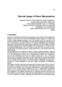
where M and C are 22 inertia and Coriolis matrices, respectively and u is the generalized torque vector which consists of the torques applied by the joint actuators [9], [10]. The elements of angular position vector denoted by q   1  2 T are shown in Fig. 1. The masses of the links, m1 and m 2 are assumed to be concentrated at the end points. The inertia and Coriolis matrices can be obtained from the geometry displayed in Fig. 1 as

    2 cos  2 M     cos  2

   cos  2    

(19)

  (21   2 ) sin 2  , 0 

(20)

and

 0 C  sin   2  1 where

  (m1  m2 )a12 ,

  m2 a 22 ,

  m2 a1a2 .

(21)

y

a2 a1

m2

2

m1

1

x

Fig. 1. Two-link robot manipulator

Let us define the state vector for the manipulator dynamics as



x  x1T x T2 with



x1   1 1



T



T

(22)



x 2   2 2



T

.

(23)

After straightforward manipulations, it is possible to show that the dynamics in (18) can be represented by a quasi-linear model as [11]

x 2 (t )  A(x(t )) x 2 (t )  B(x(t )) u(t ) .

(24)

In (24), the state and input matrices turn out to be

A  M 1C 

1   (   1 cos  2 )  sin 2  D (1    2 1 cos  2 )  sin 2

  (21  2 )  sin 2    (    cos  2 )( 21   2 )  sin 2 

(25)

and

B  M 1 

   2 cos  2  1 .  D    2 cos  2     2 cos  2 

(26)

With D  det M     2 cos 2  2 . 3.2 A Quasi-linear Model Although (23) is written in a linear state-space model format, its right hand side consists of, in fact, terms that are nonlinear in the state variables. Nevertheless, if x(t ) is available, the matrices A and B can be treated as known time-varying quantities. Hence, as far as fault-monitoring purposes are concerned, (24) can be used as a time-varying linear model to check if the system is operating in fault-free condition or not.

As a matter of fact, states can be obtained by measurements, which may be subject to noise and random disturbances. Therefore, we consider a measurement equation such as

y(t )  x(t )  e(t ) ,

(27)

where the measurement noise, e(t ) , is assumed to be a Gaussian zero-mean continuous-time white-noise vector. Since only y (t ) is available from the system, we need to derive a system equation where A and B matrices are expressed as function of y (t ) , rather than x(t ) . In other words, (24) must be written as

x 2 (t )  A( y(t )) x 2 (t )  B( y(t )) u(t )  ε(t ) ,

(28)

where ε(t ) is the equation error due to using y (t ) in evaluating A and B, instead of x(t ) . That is,

ε(t )  A(x(t )) x 2 (t )  B(x(t )) u(t )  A( y(t )) x 2 (t )  B( y(t )) u(t ) .

(29)

Note that, ε(t ) would be zero if the actual values of the states were available. So, using (27) in (24), we obtain

x 2 (t )  A( y(t )  e(t )) x 2 (t )  B( y(t )  e(t )) u(t ) .

(30)

The elements of A and B depend on x(t ) in a nonlinear and quite complicated way as given in (23), (25) and (26). Therefore, it is practically impossible to obtain a complete description of the stochastic process ε(t ) . Nevertheless, the right hand side of the (30) can be approximated by an expression that depends on e(t ) in a linear way. That is,

x 2 (t )  A( y(t )) x 2 (t )  B( y(t )) u(t )  G( y(t ), u(t ))e(t ) .

(31)

In order to obtain such a description one can use a Taylor series expansion of the right hand side of (30) around e(t )  0 (or y(t )  x(t ) ) and neglect the terms with orders higher than one. After straightforward but tedious derivations [11], the elements of

g G   11  g 21

g12 g 22

g13 g 23

g14  g 24 

(32)

turn out to be as follows:

g11  0 g12 



(33)



1  sin y 21  0.5 2 sin(2 y 21 )  2 y 22 sin y 21 Dy

(34)

g13  



 2 sin(2 y 21 ) D y2

 0.5 2 sin(2 y 21 )   (   ) sin y 21(2 y12  y 22 )  u1  (    cos y 21 )u 2 

 Dy



(35)

 cos y 21 /    cos( 2 y 21)  y12   cos y 21(2 y12  y 22 ) y 22  sin y 21 g14 

y 22 sin y 21 Dy

g 21  0

g 22 

g 23  

1 Dy

  2  sin y 21 y12 sin(2 y 21 )  2 y 22 sin y 21   2  

 2 sin(2 y 21 ) D y2

(36) (37) (38)

[(  2 ) y12   (1  y 22 )] sin y 21  0.5 sin(2 y 21 )

 (    cos y 21 )( u1  2u1 )  u 2 



(39)

1  2  2 cos( 2 y 21 )[(1  0.5 y 22 ) y 22  1]   cos y 21 ( 2 y12  y 22 ) y 22 Dy  3 sin y 21  (y12   ) y12 cos y 21 

g 24  

1 Dy

  2   sin y 21  sin(2 y 21 )  y 22 ,  2  

(40)

where D y     2 cos 2 y 21 . Note that the elements of G depend not only on the measured state (y) but also on the elements of the input vector u. Evidently, having the state measurements y (t ) at hand, (31) can serve as a quasilinear model to conduct a CUSUM test based on Kalman filtering as described in the previous section.

4 Simulation Examples In this section, typical results from extensive simulations, which have been done to validate the approach outlined above. The parameters for the manipulator are chosen as given in [12] for the two-link SCARA-type direct drive robot arm manufactured by IMI. For the sake of brevity, we are omitting a list of parameter values. Three types of changes in the changes are considered. These are sensor biases, actuator torque biases and the payload changes. Note that the first two of them can be represented as

additive signals at the output and system equations, respectively; whereas the third one in fact causes a change in the dynamics of the arm. The robot arm is assumed to be controlled by a classical PID controller and following a trajectory described by

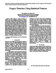
 1   2  0.8 sin t .

(41) 3 This joint angles result in a motion where the end effector of the arm is following a path as shown in Fig. 2, back and forth. Whenever a fault is simulated it is introduced at t  2 sec , until when the system is running under the nominal mode. The dynamics for the fault-free and faulty modes of operations can be described as follows:  Normal mode: x 2 (t )  A( y(t )) x 2 (t )  B( y(t )) u(t )  G( y(t ), u(t )) e(t ) (42) y (t )  x (t )  e(t )  Sensor bias: x 2 (t )  A( y(t )  d s ) x 2 (t )  B( y(t )  d s ) u(t )  G( y(t )  d s , u(t )) e(t )

y ( t )  x ( t )  d s  e( t )  Torque bias: x 2 (t )  A( y(t )) x 2 (t )  B( y(t )) (u(t )  d a )  G( y(t ), u(t )  d a )e(t )

y ( t )  x ( t )  e( t )  Payload change: x 2 (t )  A f ( y(t )) x 2 (t )  B f ( y(t )) u(t )  G f ( y(t ), u(t )) e(t )

y (t )  x (t )  d  e(t )

(43)

(44)

(45)

A sensor bias of 0.2 is assumed to occur in the measurement of the position of the first joint, i.e., d s  0.2 0 0 0 . In simulating an actuator fault, on the other hand, a fault on the actuator of the second joint is considered such that the torque delivered to the joint is decreasing by 0.1 Nm, i.e., d a  0 0.1 . Further note that a change in payload corresponds to a change in the mass of the second link, m 2 . An overload fault is considered where the link mass is increasing 6 kg beyond the nominal value. The matrices A f , B f and G f in (45) are to be evaluated under this faulty condition using (25), (26) and (32)–(40). The values estimated by Monte-Carlo simulations based on 100 runs for different types of faults are presented in Tables 1, 2 and 3. One can immediately note the classical ADD-MTBFA tradeoff comparing the estimates for different thresholds. Namely, increasing the test threshold improves the false alarm performance, nevertheless, also causes extra delay in detection. It is also interesting to observe the monotonicity of the detection delay with respect to the change magnitude, in detecting sensor and actuator biases. Even if the after-change hypotheses are based on the assumption that d s1  0.2 and d a1  0.1 for the sensor or actuator biases, respectively, larger changes can be detected as well, even faster. This suggests that the detection mechanism can be designed so as to detect the minimum relevant bias.

0.5

y (m) 0

-0.5 0.2

0.3

0.4 x (m)

0.5

0.6

Fig. 2. Trajectory of the end effector

On the other hand, the false alarm times in Tables 1–3 may seem to be low if one considers the potential applicability of the CUSUM test in practice. However, we should note that the thresholds are chosen low in order to make simulation time reasonably small and facilitate a Monte-Carlo analysis. It can be observed from (10) and (11) that the detection delay depends, roughly speaking linearly on  , whereas the MTBFA is increasing exponentially with increasing test threshold. Therefore, practically meaningful false alarm rates can be obtained at the expense of small increases in ADD by choosing larger test thresholds.

Table 1. Estimated ADD and MTBFA in detecting sensor biases

Test threshold MTBFA (sec) ADD (sec)

d s1  0.1 d s1  0.2 d s1  0.3 d s1  0.4

  2.5

  5.0

  6.0

50.5 0.556 0.493 0.441 0.403

120.2 0.615 0.537 0.497 0.461

126.7 0.723 0.566 0.511 0.470

Table 2. Estimated ADD and MTBFA in detecting actuator biases

  2.5

Test threshold MTBFA (sec)

ADD (sec)

d a1  0.1 d a1  0.2 d a1  0.3 d a1  0.4 d a1  0.5

78.9 0.512 0.245 0.153 0.116 0.108

  5.0 176.8 0.572 0.291 0.155 0.130 0.113

  6.0 180.5 0.580 0.296 0.156 0.132 0.115

Table 3. Estimated ADD and MTBFA in detecting payload changes

Test threshold MTBFA (sec) ADD (sec)

5

  2.5 19.8 0.511

  5.0 64.7 0.591

  6.0 91.6 0.697

Conclusions

In this work, we have considered application of statistical tests for detecting faults or dynamical changes in robot manipulators. A continuous-time analog of the wellknown CUSUM test has been used to detect biases in the sensors and actuators as well as dynamical changes like payload changes. The detection mechanism uses the estimation errors of Kalman filters, each of which is based on the before- and afterchange operation modes. Measurements of the joint positions and velocities are assumed to be available. To obtain a quasi-linear description of the plant, which is appropriate for linear filtering, a Taylor series expansion of nonlinear dynamics with respect to the measurement noise is considered. The first order terms obtained from such an expansion are used to approximate the plant. The work in [7] following that of [13] on the metrics of the increments of the CUSUM test suggest that the CUSUM test is robust with respect to modeling errors and, hence the test performance should not be effected seriously by neglecting higher order terms. Regarding possible further directions of research, continuous-time statistical tests, their properties and performances certainly deserve more investigation, since they may result in detection mechanisms that require simpler hardware in some cases. One interesting point in this context is that the approximations in (10) and (11) are due to the neglecting the overshoot of the test statistics beyond the threshold when an alarm is raised. Their continuous-time analogues will turn out to be exact equalities. To keep the analysis more clear, we have limited ourselves to the case where the hypotheses before and after the change are known. Although the simulations suggest that in some cases only a minimum level of change which has to be detected needs to be known, the approach outlined above can be extended to statistical tests suitable for detecting changes towards unknown hypotheses [2].

References 1. Patton, R. J., Frank, P. and Clarke, R.: Fault Diagnosis in Dynamic Systems: Theory and Applications. Prentice-Hall, Hemel Hempstead (1989) 2. Basseville, M. and Benveniste, A.: Detection of Abrupt Changes in Dynamical Signals and Systems. Lecture Notes in Control and Information Sciences, Vol. 77. Springer-Verlag, Berlin (1986) 3. Basseville, M. and Nikiforov, I. V.: Detection of Abrupt Changes: Theory and Application. Prentice-Hall, Englewood Cliffs (1993)

4. Kerestecioğlu, F.: Change Detection and Input Design in Dynamical Systems. UMIST Control Systems Centre Series, Vol. 1. Research Studies Press, Somerset (1993) 5. Lorden, G.: Procedures in Reacting to a Change in Distribution. Annals of Mathematical Statistics. 42 (1971) 1897–1908 6. Page, E. S.: Continuous Inspection Schemes. Biometrika. 41 (1953) 100–115 7. Zhang, X. J.: Auxiliary Signal Design in Fault Detection and Diagnosis. Lecture Notes in Control and Information Sciences, Vol. 134. Springer-Verlag, Berlin (1989) 8. Meditch, J. S.: Stochastic Optimal Linear Estimation and Control. McGraw-Hill, New York (1969) 9. Craig, J. J.: Introduction to Robotics: Mechanics and Control. Addison-Wesley, New York (1989) 10. Lewis, F. L., Abdalla, D. M. and Dawson, D. M.: Control of Robot Manipulators. Macmillan, New York (1993) 11. Nalbantoğlu, B. S.: Fault Detection in Robot Manipulators by Using Statistical Tests. M.Sc. Thesis, Boğaziçi University (1997) 12. Direct Drive Manipulator R&D Package User Guide. Integrated Motions Incorporated, Berkeley (1992) 13. Baram, Y. and Sandell, N. R.: An Information Theoretic Approach to Dynamical Systems Modelling and Identification. Proc. IEEE Conference on Decision and Control, New Orleans (1977) 1113–1118.