point, the characteristics of the Serrone fault resemble those described by Wallace .... Barrientos (1986) to account for features of the 1983, Borah Peak, Idaho, ...
Bulletin of the Seismological Society of America, Vol. 79, No. 3, pp. 690-710, June 1989
FAULT PARAMETERS AND SLIP DISTRIBUTION OF THE 1915 AVEZZANO, ITALY, EARTHQUAKE DERIVED FROM GEODETIC OBSERVATIONS B Y STEVEN N . W A R D AND GIANLUCA R . VALENSISE ABSTRACT
This paper analyzes static surface displacements associated with the Avezzano, Italy, earthquake (Ms -- 6.9) of 13 January 1915. The Avezzano event locates on a shallow normal fault centered in the Apennine mountains near a Quaternary tectonic depression named "Conca del Fucino." The 1915 earthquake is the only sizable event to have occurred in the area for at least a millennium, although many Holocene and Quaternary faults can be recognized in the field. Awareness of the seismic potential of the Fucino region has heightened in recent years with the outward expansion of metropolitan Rome (80 km southwest). Because of a fortuitous pre-earthquake leveling survey near the fault in the mid 19th century, good quality geodetic data exist that illuminate details of the 1915 rupture. We modeled the faulting using both uniform (USP) and variable (VSP) slip planar dislocations. The best fitting focal mechanism includes pure dip slip on a plane striking 135 ° and plunging 63 ° to the southwest. This fault geometry is consistent with surface scarps and the broad scale tectonics of the region and is common to several large earthquakes of the south-central Apennines. The USP analysis estimates fault length, width, slip and moment to be 24 km, 15 km, 83 cm, and 9.7 x 10 le N-m, respectively. Numerical simulations indicate that residuals left in the uniform slip model are not entirely random and represent systematically unmodeled features of fault slip. VSP models of the earthquake significantly reduce the USP variance and reveal a broad two-lobed slip pattern, separating a central region of low moment release. New formulations detailing the relationships between VSP and minimum model norm solutions to underdetermined inverse problems are presented as well as concise statements dealing with the intrinsic and combined resolving power of a geodetic network. INTRODUCTION
On 13 January 1915, a catastrophic earthquake occurred near Avezzano, 80 km east of Rome. The epicenter was located in a Quaternary tectonic depression called "Conca del Fucino," a name reminiscent of the Roman lake "Fucinus Lacus" that formerly occupied the site. The large magnitude of the earthquake (M~ = 6.9), the inadequate quality of building construction, and unfavorable local conditions conspired in destroying nearly every structure in the area. From a historical perspective, the earthquake was unexpected, although neotectonic features near the epicenter show evidence for repeated events of similar displacement. Geodetic leveling traverses encircled the old lake bed in 1862 and 1917 and document the 'co-seismic' (1917 to 1862) vertical deformation due to the earthquake. Despite the age of these geodetic surveys, the flatness of the topography permitted measurement precisions not significantly worse than those obtained with modern techniques. In this paper, we investigate details of the Avezzano faulting as evidenced through its surface movements. For this, we employ classical uniform slip models of earthquake faults as well as more recently developed models which include spatial variability of slip. HISTORICAL
SETTING
The epicentral region of the 1915 event has been populated from ancient times. The Fucino area served as the half-way rest spot for the old travellers crossing the 690
THE 1915 AVEZZANO, ITALY, EARTHQUAKE
691
Apennines from the Tyrrhenian to the Adriatic coasts. Being an unusually flat area in a broadly mountainous region, Fucino has been agriculturally developed for almost 2000 years. In the Roman era, Fucino suffered severe floods during the rainy season due to the huge amount of water provided by karst aquifers in the surrounding mountains, the lack of natural effluents and the flatness of the surrounding shores. To mitigate the flood hazard, Emperor Claudius inaugurated an engineering project in 52 A.D. to drain excess waters into the deeper Liri Valley to the west. To keep the lake within its banks, a 5-km tunnel was excavated through the limestone, emerging at a point 8 meters below the average shore level. In the mid 19th century a longer, deeper hole was drilled on the bottom of the lake bed that dewatered the depression permanently and, in the process, created some 150 km 2 of new fertile farmland. To insure orderly delimitation of the new lands, 18 stone monuments were installed around the lake shore prior to its drainage. Holy symbols ('Madonnas') were placed on the monuments to discourage peasants from altering the surveyed positions to fraudulently expand their properties. The monuments, which still stand today, were precisely leveled in 1862 and the new lands were divided into small parcels and colonized. By 1900, the old lake became the most important agricultural site of the region. Several small villages located around the lake shore rapidly developed, the most populous being Avezzano. In contrast to surrounding regions, there was no memory of previous large earthquakes near Avezzano prior to 1915. The existence of Roman settlements in the area and the vicinity of Rome itself guarantees that any major earthquake here would have been noted by historians. Because of its rapid colonization, and lack of experience with previous damaging earthquakes (for example, L'Aquila, 30 km to the north, was partially destroyed and more safely rebuilt on at least three occasions in historical times), the Fucino area had very poor building codes. More than 33,000 casualties were attributed to the 1915 shock; of these, 8000 were residents of Avezzano (almost 80 per cent of town's inhabitants), where only one building substantially survived the event (Beal, 1915). Poor construction partially accounts for the high death toll and for a tendency to overestimate the size of the earthquake. Beyond Avezzano, significant damage was sustained within an area of 60 km radius. In Rome, 80 km west of the epicenter, the tremor was felt with intensities between VI and VII (MCS). Some historical buildings and churches located on the Tiber River alluvium suffered minor structural damage. The main shock triggered an earthquake sequence that lasted for 10 yr. The Italian seismological community was stunned by the 1915 event and several theoretical and observational studies were carried out in the following years. Early on, misidentifieation of the macroseismic epicenter with the actual source location led to a 15 km mislocation of the event, and a complex rupture pattern was invoked to explain important deviations from the normally expected macroseismic field. Most small and intermediate aftershocks were correctly located in the vicinity of the 1915 fault, while the main shock was located near Avezzano where the seismic release had the most tragic effects. The lack of historical seismicity in the area fostered the widespread belief, even among several scientists, that the lake drainage itself might have provoked the event. TECTONIC BETTING
After a major orogenic paroxysm in the upper Miocene, a tensional regime engulfed the central Apennines and the Tyrrhenian coast. Explosive volcanism accompanied the sinking of large crustal blocks and the creation of grabens of
692
STEVEN N. WARD AND GIANLUCA R. VALENSISE
regional importance on the perityrrhenic belt. In the late Pliocene-Quaternary, several smaller tectonic depressions developed in the inner part of the chain, Conca del Fucino being the most notable. These depressions are almost rectangular in shape with some slight elongation in the Apennines direction (NW-SE) and possess high rates of seismicity. Associated earthquakes are commonly shallow, dip-slip types, slipping on steeply dipping planes with a sometimes complex rupture pattern. The Conca del Fucino is bordered by at least three major tectonic lineaments (Fig. 1): the Tre Monti fault on the north and the Parasano and Serrone faults on the east and southeast. Over the past million years, 500 to 1000 m of slip on these normal faults progressively submerged the basin, closed the way for effluent waters, and created the lake (Colacicchi, 1967; Rally, 1982). The basin itself is filled by continental and lacustrine sediments up to 100 m thick and tends to deepen on the eastern side (Accordi, 1975). The Serrone fault was reactivated by the 1915 event (Serva et al., 1986) and exposed a 50 cm high white ribbon of fresh limestone surface along its southernmost section. In the central and northernmost sections, the rupture was expressed in a straight, though discontinuous, scarp outcropping in unconsolidated sediments for almost 15 km along the lake shore. The visible southern section of the Serrone fault reaches heights of 15 m and displays a decreasing degree of smoothness from bottom to top. Slickensides and grooves suggest that the fault was built up through numerous slip events similar to the 1915 earthquake, recurring perhaps every 1000 yr or more (Progetto Finalizzato Geodinamica, 1986). From a morphological standpoint, the characteristics of the Serrone fault resemble those described by Wallace (1984) for the Pleasant Valley, Nevada, earthquake of 1915 (Ms = 7.7). Geomorphological observations, such as the existence of parallel faults northeast of the basin (Parasano fault), the distribution of uplifted terraces, and the shape of the lake's eastern shoreline, reinforce the suggestion that the 135 ° strike of the reactivated portions of the Serrone fault is representative of the strike of the 1915 rupture. The footwall of the Serrone fault contains undulations of 10 to 20 m wavelength, elongated in the down-dip direction. The axis of these bulges constrain the fault rake better than slickensides, which can be abnormally enhanced by weathering and are sometimes confused with other segmentation trends. Based on field observations, the 1915 dislocation appears to be virtually pure dip slip, although secondary faults exposed at the base of quarries excavated in front of the main fault sometimes do show a minor lateral-slip component. THE GEODETIC DATA The 18 monuments set on the shoreline before the drainage were surveyed in 1862 by a French company under contract of the Italian Government. The postearthquake survey was planned for 1915 by the Italian Instituto Geografico Militaire (IGM), which still serves as the primary geodetic governmental agency. The crew was lead by Loperfido (1919) who, just a few years before, had carried out a similar survey near the Messina Straits (Southern Italy), which had been badly hit by a Ms = 7.0 earthquake in 1908 (Loperfido, 1909). The impending world war delayed the beginning of the field operations until 1917 (Loperfido was also a ballistic teacher in the Italian Army). Because of the planarity of the route, the survey did not present any special difficulty, except for a few benchmarks that were found damaged by the earthquake. Two major concerns must be faced when comparing the 1862 and 1917 surveys: the stability of nonstandard benchmarks and the precisions of the levelings. These
693
THE 1915 AVEZZANO~ ITALY~ EARTHQUAKE
LEGEND:
r
I~,
.
~
C,
5?a\Zq
5
:
z
-
FIG. 1. (Top) Location map of the epicentra] region of the ]915 Avezzano earthquake. Legend entries are: 1) Old Lake :Bed, 2) Notab]e Quaternary and Holocene faults, 3) Scarp of 1915 event, 4) Roman Tunnel, and 5) Benchmark sites. (Bottom) Profile of the 1917 through 1862 vertical elevation changes projected along a llne perpendicular to the Serrone Fault. The zero level is arbitrary. Total variance in the data is 1.4 m 2.
A
8
+20 u
~lB
o
16
................... # . . , ~
2:
Ld
= -20 u
Is ........... - ~ ..........................................................................
1
2
#
#
I~
~
g#
cE
[3
-J
o_ -LID
oo
-
_
o
]0
-BO
5 #'A;"
~k
#~k7
II
8
#
I
16
12
I
12
I
I
I
8
DISTANCE
I
L1
(KM)
I
I
O
I
[I
694
STEVEN N. WARD AND GIANLUCA R. VALENSISE
concerns are not totally reconcilable because part of the records of the French survey were lost in the collapse of the committing agency in Avezzano. We have several reasons however, to be optimistic with regard to the accuracy and stability of the net until 1917: 1. the b e n c h m a r k s were deliberately placed within 3 to 5 cm of the free level of the lake. This natural equipotential surface thus formed an ideal datum for the entire network; 2. the surveys followed a completely plane route, systematic topographic or refractive index errors are not expected to contaminate the data; 3. the surveys are closed loops which allowed closure error checks; 4. most of the network overlies massive limestones and coarse-grained fan deposits which are expected to be free from compaction effects. 5. the 1917 survey was carefully performed and the original position and orientation of b e n c h m a r k s suspected to have suffered vertical displacements due to soil compaction or fluid removal were accurately checked. T h e b o t t o m of Figure 1 plots the 1917 to 1862 change in elevation at the 18 b e n c h m a r k s projected along a line trending southwest-northeast. Co-seismic deformation is characterized by a 60 cm subsidence of the northeast section of the lake bed relative to its opposite shore. An asymmetric p a t t e r n of surface collapse like this is typical of shallow tensional faulting on a steeply dipping plane. Pro-rated r a n d o m error in elevation differences between the 1862 and 1917 closed loop surveys accumulates like
(~(l)
4~s62 + =
2 G1917
2~ 1 < L/2 ~/2(L - l ) / L l > L/2
(1)
(Bomford, 1971), where L is the length of the route and ~1s62,1917are the respective uncertainties in elevation between the beginning and midpoint of the loop. We will assume t h a t alS¢2 = 0.05 m and a1917 = 0.02 m. T h e 1862 uncertainty represents the quoted precision goals of the French survey. T h e 1917 uncertainty is consistent with the t h e n existing standards of the International Geodetic Commission (Loperfido, 1909). T h e total squared r a n d o m error for N stations at distances In is E 2 = ~ =N z a2(l~). For a regular spacing Al among the 18 b e n c h m a r k s distributed around the 50 km of the old shoreline, l~ = (n - 1)AI, L = N A l, and
[
~__ ( n -
1)+
2 + ~917)N/2 = 0.026 m 2. = (als6~
(2)
Total signal to noise ratio for the Avezzano data set is S N R = ~, ui2/E 2 = 54. MATHEMATICAL APPROACH T h e forward problem in analyzing leveling data considers the surface deformation resulting from slip on spatially finite faults. T h e vertical displacement u ( r ) at a point r on the E a r t h ' s surface can be described as u(r) = ~ K ( r , r ° ) r h ( r °) d r °, JA
(3)
THE 1915 AVEZZANO, ITALY, EARTHQUAKE
695
where f d r ° covers all points on the fault surface A, and rh(r °) is moment density, a function of position. The kernel K(r, r °) is a function of specified fault parameters (strike, dip, and rake) and the relative positions of r and r °. Ward and Barrientos (1986) give K(r, r °) for the simple case of a uniform, nongravitating half-space. Equation (3) is perfectly general, however, and kernels can be computed under less restrictive conditions with a corresponding increase in effort. In practice, rh(r °) is discretized into N elementary sources and the data are composed of M observations. Equation (3) reduces to N
u(ri) = ~ K ( r i , r2°)m(ri °)
(4)
j=l or N
u(rl) = 2 /~(ri, rj°)s(rj °) j=l
(5)
if each source is associated with fault area 5Aj and an unknown slip s 2. A variety of inverse schemes can be applied to (5) to estimate sj from u(rl) once the fault mechanism and the fault surface have been specified. Unlike the linear formulation for fault slip, however, procedures to determine these latter parameters are highly nonlinear. As a consequence, tradeoffs between uncertainties in fault mechanism and shape and uncertainties in the determined slip pattern are difficult to address formally. Mostly we rely on forward tests and experience. UNIFORM SLIP PLANAR ( U S P ) FAULTS
The first step in our approach finds the best fitting uniform slip, plane rectangular fault. The best USP fault not only provides a standard with which to compare more complex models, but it also supplies a fault orientation and slip direction which must be specified prior to inversion of (5). The complete formulation of the USP model involves ten unknowns: strike, dip, and rake angles; fault slip; length alongstrike and width along-dip; the x, y and z position of a fault upper corner; and a static baseline correction u0. The degree of linearity between generated surface displacements and the ten USP parameters is variable. The slip and baseline corrections are totally linear parameters, whereas fault length, width, and depth are quasilinear. The influence of the remaining five is unpredictable. Because of the variable degree of linearity, it is unlikely that all 10 parameters can be recovered simultaneously in an unrestricted inversion. Fortunately, other information is usually available which can constrain certain fault parameters without introducing undue bias. For example, the strike of many shallow earthquakes is known within a few degrees from their surface expression. By constraining some parameters thought to be more certain, recovery of the remaining parameters is possible. Two different techniques are used in USP parameter estimation: a trial and error search and a Levenberg-Marquardt linearized inversion. The trial and error method involves brute force, but it can cover a large range of model space and is not affected by nonlinearities. The analytical inversion is more elegant, converges faster if started near a minimum, and through adjustable damping can partially account for the variable linearity among the 10 unknowns. We have no preference between the
696
S T E V E N N. W A R D A N D G I A N L U C A R. V A L E N S I S E
approaches; both can give adequate results. The first technique is used to rapidly scout solutions, while the second searches for the best-fitting values in a restricted parameter space. The Avezzano rupture created a well observed surface scarp that permits the strike, slip angle, and southernmost upper corner of the fault to be assigned with confidence: strike, 135°; slip angle, 270°; southernmost corner, at 1000 m depth near the abandoned village of Sperone (Fig. 1). The remaining parameters from the USP inversion are: dip angle = 63 °, fault l e n ~ h = 24 km, fault width = 15 kin, slip = 0.83 m and Uo = -3.5 cm. The geodetic moment of the USP model is M0 = 9.7 x 10¹⁸ N m for h = t~ = 3.23 x 101° Pa. Figure 2 contours the vertical displacement associated with the best USP model and contrasts observed versus theoretical uplifts in cross section around the survey loop. Although the best USP fit appears reasonable, the total residual variance is 0.152 m 2, about six times larger than the estimated uncertainty in the data. We presume that the excessive USP variance is a systematic discrepancy resulting from the restriction of uniform slip. VARIABLE SLIP PLANAR (VSP)MODEL Variable slip analysis of geodetic leveling data was first introduced by Ward and Barrientos (1986) to account for features of the 1983, Borah Peak, Idaho, earthquake that were left unexplained by USP models (Stein and Barrientos, 1985). Barrientos (1988) later applied a similar approach to the 1985 Central Chilean earthquake. In matrix form, the linear problem describing the moment distribution (4) is u
( M x 1)
=
K
m
(MxN)
(6)
( N x 1)"
R
8
+20
g ~ -20
-60
f
l
~
~
l
J
~
J
÷20 /
o 4 ....................................
.................
................
20 '
. . . . .
5
KM 16
12
8 OI STRNCE
q
0
[KN)
FIG. 2. (Left) C o n t o u r m a p of vertical surface d e f o r m a t i o n at 0.1 m intervals for t h e best fitting rectangular U S P fault. L i g h t dots r e p r e s e n t t h e surface projection of locations of nonzero slip. (Right, top) Observed (stars) a n d calculated (circles) elevation c h a n g e s for t h e survey loop projected on A-B. T h e zero level here is fixed by t h e inversion. (Right, bottom) Elevation residuals of t h e U S P model projected along A-B. T h e U S P model fits 90 per cent of t h e data variance, b u t h a s residuals about six t i m e s greater t h a n t h e e s t i m a t e d survey noise.
697
THE 1915 AVEZZANO, ITALY, EARTHQUAKE
In VSP models, the n u m b e r of elemental sources distributed on the fault (N = several hundred) generally far o u t n u m b e r the available data (M --- dozens). Provided t h a t (6) is consistent ( K K - t u = u), a complete set of exact solutions can be formed as
m = K-lu
+ (I -- K - I K ) m ~ ,
(7)
where K -~ is any matrix satisfying K = K K - t K and mm is any (N x 1) vector. T h e second t e r m in (7) represents the class of slip distributions t h a t produce no vertical deformation at any b e n c h m a r k in the net. For arbitrary K -~ and ram, exact solutions (7) will be extremely ragged, frought with large and narrow peaks of positive and negative slip. To subdue physically objectionable aspects of an arbitrary solution (7), a variety of smoothness constrains have been formulated. T h e most common is the minimum model norm (MMN) t h a t assumes (I - K - t K ) m m = 0 and singles out K -~ = K T ( K K T ) -1. This is equivalent to expressing the N unknown moments as a linear sum of M basis functions, m = KWe. T h e M basis functions forming the columns of K w are fairly smooth and were t e r m e d sensitivity kernels by Ward and Barrientos (1986). M M N solutions have the properties, E2(mMMN)
=
II
K m M M N -- U
fi
=
0;
(8)
min li mMMN [0, and represent the smallest perturbation about m = 0 for which prediction error EZ(m) vanishes. Since (6) is consistent, 1TIMMN is unique even if K K w is singular. Figure 3 illustrates the M M N solution on an 18 by 36 km segment of the best U S P plane. T h e M M N approach is linear and can give unique solutions; unfortunately,
-10
S E: 0.00[30
.
...........
.'..-~ < - ~ -z- -- _, ,- .., / ',t, , , ' / / / / / ~ ' ~ . ~ ' ~ . - ;.;,~.-*;'" V/~.',;..:..'/~/'.'; /I
/111
P
I
(b)
\~ ~
I
I
"~.///./.~
",";.,.,;,,,.,'" " ~
\
.......
"
"
I
(c
[
I
6
KM
FIG. 9. Illustration of t h e effect of r a n d o m survey noise on t h e V S P slip pattern. (a) T h e m e a n of 50 inversions which included survey errors of t h e type given in equation (16). T h e contour interval is 0.3 m a n d t h e initial contour is 0.15 m. D a r k s t a r s m a r k t h e point of closest approach of t h e fault plane a n d t h e 18 b e n c h m a r k s . H a s h e d areas denote portions of t h e fault within the 15 cm contour which have a slip m a g n i t u d e more t h a n two (b) or four t i m e s (c) its s t a n d a r d deviation. Slip at an average point on the fault exceeds its s t a n d a r d deviation by about a factor of 3. It is unlikely t h a t t h e two lobes or t h e shallow k n o t s of slip result from r a n d o m error p r e s e n t in the data.
704
STEVEN N. WARD AND GIANLUCA R. V A L E N S I S E
Resolution Tests VSP slip patterns derive directly from the M sensitivity kernels in K T, which contain the physics of the problem. To understand the VSP method, the structure of these kernels must be appreciated. Figure 10 maps/~(r~, r d) over the assumed fault surface r ° for several representative benchmarks r~. Resolution kernels are relatively smooth, with one or two changes in sign and they typically peak at the point of closest approach of the benchmark and the assumed fault. Distant stations possess broad kernels centered deep of the fault (Figure 10a, h, i), while near-in stations possess peaked kernels centered shallowly on the fault (Figure !0c through f). Consequently, information contained in uplift data from distant and near-in benchmarks will map into wide and concentrated slip patterns respectively. Because the VSP solution is the positive part of a simple sum of the columns of K w, amplitude and length resolution should decrease with depth, Intrinsic Geodetic Resolution The ability of a geodetic leveling survey to resolve slip on a specified surface can be addressed through one of the properties of VSP solutions. For arbitrary m given on the fault, its VSP projection (15) is
[(Kan)-~Km],o~
nlSpos =
(17)
If m is a delta function at the ith source point r/°, and ~ includes all points r 9 on the fault where J r~ ° - ri°l < l, then the unitless quantity
• .
• ~ ' - ~ ' ~ ' . " ,.
i ~
~,
~
,'
~
'
~
I ', ', '6,'~-- *,','/.:~' ', ', BM
1
(a) •
I
7
~.
*
1 5
,l~',
"/
.0017
BM
.0812
""~"~'~'~'"~""
(g)
-x
/ .
.5
(b)
/
' ,' ,,'~"c_".:,',' ': I ', *'
'~
- ~ , ,
*
~ 1
BM
~
"" ."
.0058
* .0045
"~'~"* "
I
(d)
•
BM
,,E,
, ",'-:L-*",~*,'
"-
I
BM
,
,
9
BM
I
.0915
/,'.,,;,:'~,':-: 16 kin, A x no longer changes noticeably. Slip features of this size can be detected anywhere over the specified surface. An admirable aspect of the inversion is that moment released at points unilluminated by the net is largely ignored rather than mismapped elsewhere. Combined Geodetic Resolution Equation (18) and Figure 11 provide useful insights into the intrinsic resolving power of a leveling network. Often, however, it is desirable to formulate a measure of resolution which accounts for the combined effects of the net geometry and the quality of the survey. One measure of the spatial resolving power of N stations r~ in a geodetic net comes from the RMS sensitivity kernel
R(r°) =
-~ 2 K2(r~, r°)
(19)
i=1
evaluated at points r ° on the fault. Introducing R (r °) into the quantity L m i n ( r O) =
I
I
I
i
~
i
"~ / / ~ / s t a i n )
V
r
I
i
(20)
i
i
i
~
(o)
L=
~ KM
(b)
L=
2 KM
(c)
L=
(d)
L= 4~:~
(e)
L= 8 K M
(f)
L=IG
I
5 KM
KM
FIG. 11. Contour map of intrinsic geodetic resolution A~(r~°) (equation 18) for l = 1, 2, 3, 4, 8, and 16 km. Intrinsic geodetic resolution quotes the resolvability of slip features of size I without regard to the precision of the survey. The box is 18 by 86 kin. Contours are 0.25, 0.50, 1.0, and 2.0. The outermost contour encloses the area in which slip features of dimension l can be resolved at the 25 per cent level. Larger slip features can be seen deeper on the fault. Note the slight hole in intrinsic resolution in the center of the network.
706
STEVEN N. WARD AND GIANLUCA R. VALENSISE
produces an estimate of the scale length of resolvable slip features from a survey of a specified precision. In (20), E is the m e a n survey error ~/E2/N (see equation 2) and s m~' is some characteristic slip. As E grows in less precise surveys, the size of resolvable features m u s t increase for a fixed characteristic slip, or, characteristic slip m u s t increase on resolvable features of fixed size. Figure 12 contours L m~" in k m for s m~" = 1 m a n d / ~ a p p r o p r i a t e for the Avezzano survey. Again, the scale length of recoverable features is seen to increase with depth on the fault a n d distance f r o m the net. N e a r the surface, 1 m slip patches i k m wide should be resolvable above the survey noise. T o w a r d the b o t t o m of the fault, 1 m slip features would have to be 10 to 12 k m wide to be discerned. C o m b i n e d resolution lengths for I m slip in the center of the fault is 5 or 6 kin, so slips as small as 0.25 m over the 10 to 12 k m wide area in the center of the net should be observable. T h e central p a t c h of low slip in Figure 7 is thus likely to be real, despite the s o m e w h a t lower intrinsic resolution in this area noted in Figure 11.
Patch Tests P a t c h tests are a simple m e t h o d of evaluating resolution. P a t c h e s of unit slip are distributed on the fault a n d (17) is employed to determine their V S P projections. Figure 13 shows the V S P slip p a t t e r n s from nine, 6 k m by 6 k m blocks of unit slip scattered at various sites. P a t c h tests visually reconfirm the more elegant s t a t e m e n t s of resolution in (18) a n d (20). Sources within the net are b e t t e r resolved b o t h in length a n d a m p l i t u d e t h a n are patches toward the edges of the fault. Note t h a t the p a t c h in the center of the net (Fig. 13e) is well reproduced. T h i s again suggests t h a t the central area of low slip in Figure 7 is likely to be real a n d not due to poor resolution. All of the results from these stability a n d resolution tests indicate t h a t the V S P technique consistently produces physically reasonable models which neither overinterpret or ignore resolvable i n f o r m a t i o n contained in geodetic data. For high signal-to-noise data sets, we have confidence in the verity of the d e t e r m i n e d slip p a t t e r n for points within the sensitivity domain of the net.
NW
SE
//////(LL _