Fault Prediction Capability of Program File's Logical-Coupling Metrics. Syed Nadeem Ahsan and Franz Wotawa. Institute for Software Technology, Graz ...
Fault Prediction Capability of Program File’s Logical-Coupling Metrics Syed Nadeem Ahsan and Franz Wotawa Institute for Software Technology, Graz University of Technology Inffeldgasse-16b/II, 8010-Graz, Austria {sahsan,wotawa}@ist.tugraz.at Abstract—In the recent years several research studies reveal that the presence of logical couplings among source files, make the structure of the software system unstable, and any new changes in the coupled source files become more error prone. Hence, logically-coupled source files are strong candidate for restructuring. To identify those source files, which are logically coupled, metrics and software visualization techniques have been used. We therefore in this paper, propose an approach to compute a set of eight metrics, which measure logical-couplings among source files. These metrics are based on the historical data of software changes that comprise two or more source files. To validate that our propose set of metrics is highly correlated with the number bugs and are more capable to construct bug prediction model, we first find the correlation of logical-coupling metrics with the number of bugs, and then build machine learning based bug prediction model. To achieve our goals, we perform an experiment by extracting software evolution data from the freely available repository of GNOME project. Our experimental results show that our propose set of logical-coupling metrics is highly correlated with the number of bugs, and hence can be used to identify those source files which are candidate for restructuring. Furthermore, our experimental results show that logical-coupling metrics can be used to construct more accurate bug prediction models. In our experiment, the accuracy of our propose bug prediction model is promising i.e., 97%. Keywords-Software visualization; logical coupling; software metrics; mining software repository
I. I NTRODUCTION Software corrective maintenance, restructuring and reengineering are costly endeavor, because it is nontrivial and time consuming to identify the causes which induce defects into software systems. Therefore, before releasing a new version of a software product huge effort (e.g., code inspections, program analysis, pre-release testing) goes to ensure that there is no bugs remain in the release products of a software. These efforts could be better and well directed if we have a better understanding of what causes make the system unstable and generate defects [6]. One major cause of frequently generating software defect is modifying a program source file without prior analysis of its previous change-coupling patterns. The development scenario become worst, when developer made changes in a program source files, which is logically coupled with other source files, and programmer unintentionally forget to made changes in all the related coupled source files. Consequently, system become unstable. The possible remedy
to reduce the frequent occurrence of such scenarios, is to equip software developers with tools and techniques that provide information related to the logical coupling nature of source files. Formally, logical coupling is defined as, the implicit dependency relationship between two or more software artifacts that have been observed to be frequently changed together during the evolution of the system [4]. Logical coupling information helps to understand how the system has evolved and provides support in system restructuring. Recently, many research works have been done on logical coupling, which extracted coupling information of source files from software repository and used them to obtain a set of coupling metrics and to visualize the structural complexity of the software systems [7], [8], [3], [14]. The recent research trends in software engineering reveals that logical coupling measures are highly correlated with the number of defects [6], [5]. M. Eaddy et al. and D’Ambros et al. have addressed this issue in separate attempts, M. Eaddy et al. correlated cross-cutting concerns with defects, and D’Ambros et al. link logical coupling measures with the number of bugs. D’Ambros results reveals that logical coupling metrics are highly correlated with the number of bugs as compared to others classical set of metrics i.e., LOC, Chindamber and Kemerer metrics suite etc. In this paper we propose an approach to obtain a set of logical coupling patterns, which are related to the fixing of bugs. We obtain these patterns by mining bug-fix transactions data of source files, and use them to define a set of metrics. Our research hypothesis are, 1) The history of coupled source file’s bug-fix patterns can be used to obtain a set of coupling metrics, which are more correlated with the number of bugs. Consequently these metrics can be used to identify those source files which are candidate for restructuring. 2) Logical coupling metrics can be used to construct a regression based bug predictor models. Furthermore, logical coupling metrics can be used for the classification of source files as low, medium or high level of complexity. The main contributions of our research work are: (i) We defined a set of eight different metrics to measure the logical couplings tendency of a source file. (ii) We also performed an experiment by extracting the bug-fix trans-
action data from the software repository of GNOME OSS project, and obtained a set logical coupling metrics. We used statistical technique i.e., spearman’s rank correlation to find the correlation between logical coupling metrics and number of bugs. We found that logical coupling metrics set is highly correlated with number of bugs. The maximum obtained correlation value is 97%. We also obtained the correlation between source files level metrics (i.e., LOC, cyclomatic complexity etc.,) and the number of bugs, and compared its value with the correlation values of logical coupling metrics. We, found that logical coupling metrics out-class the classical source file level metrics. (iii) To analyze the bug prediction and classification capabilities of the logical coupling metrics, we used statistical regression and classification techniques of statistics and machine learning. In case os statistical regression we used Stepwise Linear Regression Model and Regression Model based on PCA (Principal Component Analysis). The obtained R-Square values for the two models are 95.5% and 80% respectively. Similarly in case of machine learning based classification we used J48 classifier and obtained 97% accuracy. The paper is organized as follow: In Section 2 we discuss related work. In Section 3 we describe the process to obtain the data from different software repositories. In Section 4 we describe the logical coupling patterns and logical coupling measures. In the next section i.e., Section 5, we describe in details the analysis of Sperarman’s Rank correlation. In Section 6 we discuss the bug predictor and the bug classification models. In Section 7 we discuss threats to validity. Finally in Section 8, we conclude the paper and discuss future work. II. R ELATED W ORK In the recent years, few attempts have been made by researchers to correlate the logical-coupling metrics with the number of bugs [6], [5]. However, most of the research work have been performed, which discussed the significance of logical coupling [10], [7], [16]. In this section we first discuss research works, which are related to the coupling patterns and coupling measures, while in the last paragraph we discuss the works which are related to the correlation of coupling measures with the number of bugs. The concept of change/logical coupling was first introduced by Ball and Erick [1]. They extracted the software evolution data from version control system, and used them to visualize the different cluster of source files which are changed together. Harald Gall et al. [7] developed a technique called CAESAR to identify the change patterns by identifying the logical coupling among modules across several releases of a software. Their technique find the cochange patterns among the source files of different modules. For this purpose they processed the evolution data of a software system. Their technique found dependencies among modules, they validated these dependencies by examining
the change reports. Harald Gall et al. [8] described an approach to identify the internal and external coupling among the submodule of a software system, which is based on the frequency of source file co-change pattern. They identified weak structure and recommended for re-engineering, if the submodules have a multiple external coupling. Their approach is based on three steps i.e., in the first step they identify the source file change growth, while in the second step they identify the common change patterns among the source files, and in the last step they compared classes by performing relational analysis. Breu and Zimmermann [3] processed the co-change data for aspect mining, which identifies cross-cutting concerns in a program. They identify and rank cross-cutting concerns. Zimmermann et al. [16] applied data mining techniques on software change data sets. The authors obtained information regarding which entities changed together in the past and used this information to guide the developers in case of new changes. They used pattern mining and association rules to perform the experiment. James M. Bieman et al. [2] processed those cluster of classes which are most frequently changed together. They described a method to identify and visualize classes and their interactions that are most change-prone. They measured the degree of change-proneness with the help three metrics i.e., local change proneness (related to single class change), pair change coupling (when two classes changed together) and sum of pair coupling (a class may be involved in multiple pair couplings). Martin Fischer et al. [11] extracted the software repositories data including Bugzilla bug reports and CVS log files and integrate them into an SQL database. They developed an heuristic approach to map the CVS log data to the bug reports in Bugzilla. They performed several experiments on the obtained database and identifying logical coupling among the source files based on the link of a file with the bug reports in the Bugzilla and including all the other files that also referenced the same bug report. Pinzger et al. [14] introduced a multivariate visualization technique, RelVis, that builds on Kiviat diagrams. They represent module as kiviat diagrams and logical coupling between modules as edges connecting the kiviat diagram. Kiviat diagrams are designed to visualize multivariate data such as source code and evolution metrics. Noriko Hanakawa [9] proposed a visualization technique and software complexity metrics for software evolution. They considered that the modules that have strong module coupling should also have strong logical coupling, and the system become more complex if the gap between a set of modules includes strong module coupling and set of modules including strong logical coupling is large. They developed a tool to visualize the change in software complexity metrics on time series. They tested their tools on seven different OSS project and found that the complexity metrics value is high for those softwares that have a high bugs rates.
M. Eaddy et al. [6] correlated cross-cutting concerns with defects. They performed an empirical study on three open source projects. They used the set of metrics related to the cross-cutting concerns and correlate them with defects. Their experimental results reveal that more scattered and tangled code for the implementation of a concern is highly correlated with the defect. D’Ambros et al. [5] point out that change coupling (or logical coupling) measures are highly correlated with bugs. They defined a set of change coupling metrics and used them with Chidamber and Kemerer metric suite to correlate them with the number of bugs. Their experimental results show that change coupling metrics are more correlated with bugs as compared to other metrics such as complexity metrics. They performed their experiment on three large software system i.e., Eclipse, ArgoUML and Mylyn. Their experimental results proved that the performance of bug prediction model based on complexity metrics can be improved if using change coupling measures. To keep in mind the high correlation of change coupling measures with the number of bugs, and to further validate D’Ambros approach, we designed an experiment on different data set and introduce a new set of change coupling metrics. III. DATA E XTRACTION AND F ILTERING The logical coupling’s data are obtained from software change transactions. These transactions are accumulated during the evolution of any large software system, and stored into a CVS/Subversion repository. In each software change transaction, developer’s made changes in one or more source files and commit these changes into CVS/Subversion. From these set of software change transactions data, one can easily extract the set of source files, which are committed together, and call them Coupled Source Files. Developers made software change transactions, whenever a software change request is reported into a bug tracking system like Bugzilla. Therefore, the first step is to extract the raw data from the software repository i.e., CVS/Subversion and bug tracking system i.e., Bugzilla. We therefore, downloaded Subversion log files and Bugzilla bug reports from the software repositories of Gnome open source project. The downloaded data are in html, xml or text format. Therefore, we parsed each data file and stored them into a relational database, by using an approach gave by Fischer [11]. After obtaining the data, filtering and mapping are required. In the first step, we established a link between the bug reports and the associated check-ins (commit) in the version control system e.g. Subversion. In each checkin developers make changes in the source files and save those changes into Subversion. We obtained these links by processing the log data of Subversion, and received the number of check-in transactions that are related to bug fix changes. To identify the bug fix transaction we parsed the developer’s check-in comments. If comments contain any of the following words bug fix, bug fixed, or fixed, or
Figure 1. Percentage of the selected source files, which were fixed 1-to-15 times. Like the percentage of those source files that were fixed 2-times is 17%. These source files are selected from GNOME project repository to perform the experiment.
any bug-id, and followed by 6-8 integer numbers then we considered this transaction as a bug fix transaction [11]. We also used two independent levels of confidence, i.e., syntactic and semantic level of confidence. The syntactic level is used to infer the link between change log messages and bug reports whereas the semantic level is used to validate the link by matching the bug report data, see [15]. We used this approach and defined each link with syntactic and semantic level of confidence. After identifying all the bug fix transactions and linked them with bug reports, the second step is to find the names of the source files, which have been modified in each transaction. In case of Subversion all those files, which are committed together have the same revision number. Therefore, in case of Subversion one can easily obtain the list of source files, which are changed in a single transaction. In order to perform the experiment, we downloaded 1,537 source files (c-files) from the GNOME project repository. These source files have been fixed in 2,093 transactions during 2000-2008. After downloaded the source files and their associated transactions data from subversion, we established a linked between the subversion transaction data and the bug-tracking system. We found that in our data set, the number of bug-fixed transactions associated to each of the source file is lies between 1 to 15, whereas, the distribution of source files on the basis of their number of bug-fix transactions is shown in a pie-chart of Figure 1. It is shown in the Figure 1 that in our obtained data set, 47% of the source files have only one bug-fix transaction, whereas 53% of the source files have more than one bug-fix transactions. In order to perform the experiment we selected only those source files, which are belongs to maximum 15 bug-fix transactions. However our method is also valid for any large number of transactions, but during experiment we found that most of the source files were fixed in very few transactions.
IV. P ROGRAM F ILES C OUPLING PATTERNS AND C OUPLING M EASURES In this section, we first describe the method which we used to obtain a set of bug-fix patterns of source files. Then, we formally describe a set of metrics, which we used to measure the logical-coupling tendency of source files. A. Logical-Coupling Patterns In the field of software engineering pattern mining are very common. Patterns are obtained by analyzing the history data and found that how the things have evolved. To obtain the bug-fixing patterns of coupled source files we use our own heuristic approach, which process the bug-fix transaction data related to each source file, and obtain a set of coupling patterns. These patterns are the set of source files, which have been fixed in one or more transactions. Each unique set of source files is considered as a unique pattern. Whereas, the number of transactions in which a same unique pattern has observed, is considered as the frequency of that pattern. In the following paragraph we formally describe our method which we used to obtain logical coupling patterns. Let, F be the set of source files and T be the set of bug-fix transactions. A transaction ti is a set of transactions {t1 ,t2 ,..,tk } such that fj ∈ F i.e., each fj is a source file changed in transaction ti . Let, file fp is changed in the transactions t1 ,t2 ,..,tq ∈ Tc , where Tc be the set of coupling transactions such that Tc ⊆ T. In order to find the set of source files, which have been changed together with fp in one or more transactions, we have to take the intersection of each possible combination of transactions Tc . The possible number of combinations are 2q -1, which is used to find the patterns. Consider PT={pt1 ,pt2 ,pt3 ,..pti ..ptr } be the set of patterns, where pti ⊆F and r is the number of distinct pattern. Now, in order to compute patterns from transactions T of source files F, let |Tc | = |2T -1| be the possible combinations of transactions. A pattern from Tc is given as follows: { fi | fi ∈ F ∧ ∀ t ∈ T → fi ∈ t}. Figure 2 depicts an example, which shows that how the patterns are obtained from bug-fix transaction data of a source file f1 . B. Logical Coupling Metrics Metrics are commonly used in software engineering for basic understanding and obtain a higher level views of the software. Furthermore, metrics are used for finding of design violations. In case of software evolution, metrics can be used to identify those parts of the software, which are unstable and candidate for refactoring [12]. In our experiment we defined 8 different metrics, which measures the coupling tendency of a source files, and may be used to identify those set of source files which are candidate for refactoring or restructuring.
Before formally describe the set coupling measures, once again consider the set of source files F such that fp ∈F, represent a source file whose logical-coupling patterns are need to be determined. Whereas, fc ⊆F, represents the set of logically-coupled source files with fp . Now, in our experiment an event i.e., software change transactions t, is define as, Fc (fp , fc ) = { t | t∈T ∧ fp ∈ t ∧ fc ∈ t }. Count of Coupled Source Files (COCSF): In case of COCSF metrics, we count the element of fc , where each element of fc is a source file which has been fixed with a source file fp . In simple, COCSF counts the total number of source files coupled with a source file fp i.e., | fp |= k, where k is the cardinality of fc . Coupling Patterns Count (CPC): CPC count the distinct number of coupling patterns. In the previous section, we described how to obtain the number of distinct coupling patterns. A pattern is obtained when we take the intersection of two or more transactions. If PT={pt1 ,pt2 ,pt3 ,..ptj ....,ptr } be the set of obtained patterns for source file fp , where r is the number of distinct pattern or cardinality of PT. Therefore, | CPC(fp ) |= r. Sum of Coupling Pattern Frequency (SCPF): Each pattern associated to a source file have some frequency of occurrence. Frequency is the count of the same pattern, that occurred in one or more transactions. SCPF simply add all those frequencies. If ptj ∈PT, then SCPF is given as, X SCPF(fp )= Frequency(ptj ) ptj ∈P T ∧fp ∈ptj
Average of Coupling Pattern Frequency (ACPF): ACPF add all the pattern frequency of source file fp , and divide it by the total number of patterns r. Where r > 0. X ACPF(fp )= Frequency(ptj ) / r ptj ∈P T ∧fp ∈ptj
Maximum of Coupling Pattern Frequency (MCPF): It represents the frequency value of a pattern, which is the most frequently occurred pattern of a source file fp , MCPF(fp )= Maximum(Frequency(ptj )) Sum of Coupling Conditional Probabilities (SCCP) SCCP measure the sum of the conditional probabilities of each pattern associated to a source file fp , X SCCP(fp )= p(PT=ptj , F=fp ) /p(F=fp ) ptj ∈P T ∧fp ∈ptj
Weighted Sum of Coupled Source Files having Same Parent Folder (WCSFSPF) : WCSFSPF add all the coupled source files (fc ) frequency (number of time fc coupled with fp ), such that both fc and fp belongs to the same directory or same parent folder. X WCSFSPF(fp )= Frequency(fk ∈ fc ) k
where, parent folder of fp = parent folder of fk
Figure 2. An Example to obtain a set of logical-coupling patterns for source file f1 , which were fixed 3-times in the past, and logically coupled with source files f2 ,f3 ,f4 ,f5 ,f6 . The obtained set of logical-coupling patterns of source file f1 with maximum frequency is shown in the right-most column.
Weighted Sum of Coupled Source Files having Different Parent Folder (WCSFDPF) : WCSFDPF add all the coupled source files (fc ) frequency (number of time fc coupled with fp ), such that both fc and fp belongs to the different directory or different parent folder. X WCSFDPF(fp )= Frequency(fk ∈ fc ) k
where, parent folder of fp 6= parent folder of fk C. Interpretation of Logical Coupling Metrics : In the previous section we formally defined a set of logical coupling metrics. In this section we discuss some of the important interpretation of the defined set of metrics. The set of logical coupling metrics can be categorized into three main categories, like the following metrics set i.e., COCSF, CPC, SCPF, ACPF and MCPF belongs to the category that measures coupling patterns of a source file. Whereas, metric SCCP belongs to the category, which measures the probabilistic value of a coupling patterns. Finally, the metrics set WCSFSPF and WCSFDPF belongs to the category of metrics which exploit the cross cutting concerns nature of a source file. To understand the semantic of logical couplings measure, consider the following examples, Example-1: Let we have two source files A and B. Both the source files have been changed 10 and 20 times respectively. Suppose that file A is coupled with file C in 4 transactions, whereas file B is coupled with file D in four transactions. Now, we compute their logical coupling metrics values using the relations which we have discussed in previous section, i.e., COCSF(A)=COCSF(A)=1, CPC(A)=CPC(B)=1, SCPF(A)=SCPF(B)=4, ACPF(A) = ACPF(B)=4 and MCPF(A) = MCPF(B)=4. These metrics values show that both source files have same logical coupling measures, but the values of SCCP(A)=4/10=0.4 is different from SCCP(B)=4/20=0.2. Example-2: Now, consider the example of Figure 2. Let FP={f1 } has been changed 10 times, out of which 3
times f1 were changed to fix the bug with five other source files i.e., FC={f2 ,f3 ,f4 ,f5 ,f6 }. The number of all the possible combination of bug fix transaction is 23 -1=7. Let source files f2 ,f3 and f4 have different parent folder as compared to the parent folder of f1 . Similarly, f5 , f6 and f1 have the same parent folder. Following are the set of metrics, 1) COCSF(f1 )= 5 (total number of coupled files is 5) 2) CPC(f1 )=3 (From Figure 2. the obtained number of frequent pattern) 3) SCPF(f1 )= 3+2+1=6 4) ACPF(f1 )=6/5 5) MCPF(f1 )=3 6) SCCP(f1 )=3/10+2/10+1/10=0.6 7) WCSFSPE(f1 )=2 8) WCSFDPE(f1 )=3 9) Instability=3/(3+2)=0.6 D. Source File Metrics Set In order to perform a comparison, we also computed a group of metrics, which may be used to measure the coupling tendency of C files. We selected only those metrics which are valid for source files written in C-language. Because, we performed this experiment on GNOME project data. Whereas, GNOME is mainly developed in C-language. Following are the set of classical metrics, which we used in our experiment for comparison purpose. 1) LOC : Line Of Code, which count all the executable lines of source code present in a source files. 2) FINC : File included, which simply count the syntax include present in a source file. 3) TFUNC : Total function count, which count all the functions belongs to an individual source file. 4) TFPC : Total function parameter count, which count all the function’s parameters present in a source file. 5) TRP . Total return point, which count all the returns point of each function present in a source file.
6) TCYCLO : Total cyclomatic complexity, it add all the cyclomatic complexity related to each function present in a source file. V. A NALYSIS OF M ETRICS C ORRELATION W ITH N UMBER OF B UGS In this paper our main objective is to find the correlation between the set of logical coupling measures and the number of bugs. Furthermore, for comparison purpose we want to obtain the correlation between the classical set of metrics (LOC, Cyclomatic-Complexity, etc) with the number of bugs. We therefore obtained the program source files coupling data and defined a new set of coupling measures, which we have discussed in Section III and Section IV. Now, in this section, first we discuss the statistical technique which we used to compute the correlation values, and then discuss the obtained results of our correlation values. In Statistics, correlation is a measure of association between two variables. Like, in our case these variables are the number of bugs and the source file’s metrics. The value of the correlation coefficient varies between +1 and -1. When the value of the correlation coefficient lies around 1, then it is said to be a perfect degree of association between the two variables. As the value goes towards 0, the relationship between the two variables will be weaker. Usually, in statistics, we measure two types of correlation i.e., Pearson correlation and Spearman’s rank correlation. In case of Pearson correlation we compute the degree of the relationship between the linear related variables, and both variables should be normally distributed. Therefore, Person correlation belongs to parametric statistics, where sample distribution is known. Whereas, Spearman’s rank correlation coefficient is nonparametric that does not assume any assumptions related to the distributions of correlated variables. Therefore, for Spearman’s rank correlation it is not necessary that both the variable should have linear relationships. Spearman’s rank correlation can be used if the relation between the two variable is non-linear [?]. In our experiment, we found that most of the metrics are nonlinear related with the bug count. Figure 3, depicts the scatter plots of the concern metrics versus bug count, which shows that most of the metrics are non-linearly related with the number of bugs. However, there are few metrics, which are linearly related with the number of bugs. We therefore used Spearman’s rank correlation. Following are the main reasons, 1) Spearman’s rank correlation is valid for both linear and non-linear relationships between the correlated variables, and in our experiment most of the metrics are non linearly correlated with the number of bugs 2) Since we don’t know exactly which distribution is followed by the obtained metrics data set. Therefore, performing parametric statistics i.e., using Pearson
correlation is not a valid solution. Hence, the best solution for our experiment is Spearman’s rank correlation, because it is belong to non-parametric statistics. Before computing the correlation values, we obtained the values of eight different logical-coupling metrics by using the relations which are given in Section IV-B. Similarly, we obtained the six different classical metrics, which are given in Section IV-C. Once we obtained the metrics data and the number of bugs related to each source file, then we used these data to compute the Spearman’s rank correlation values between metrics and bug counts. Furthermore, in order to find the collinearity among the metrics values, we also computed the correlation values between each pair of metrics. The obtained results of correlation are shown in Table 1, most of the logical coupling metrics are highly correlated with the number of bugs. While, in case of classical metrics set, unfortunately non of the metrics are found to be highly correlated with the number of bugs. We obtained correlation values at 0.01 level of significance. In case logical coupling metrics, the maximum obtained Spearman’s rank correlation is for SCPF and CPC metrics i.e., 0.982 and 0.938. While, lowest in case of WCSFDPF i.e., 0.343. The other metrics like COCSF, WCSFDPF, ACPF, MCPF, and SCCP have a positive and high correlation with the number of bugs, most of them have a correlation value greater than 0.65. SCPF and CPC are directly related to the number of distinct patterns. Whereas, each pattern of a source file is a distinct group of one or more associated coupled source files. It means that SCPF and CPC are directly related with the degree of scattering of a source file, and it is found in one of the experiment performed by Eaddy M. that if the degree of scattering is high then the source files are more error prone [6]. WCSFDPF, count the number of coupled file in different parent folder, therefore we can assume that this metric is measuring the cross cutting concern. Because, in case of software development, source files are normally grouped into one separate folder to perform some specific task or used for some specific concern. Therefore, if the coupled source files are belong to different parent folder folders, then it means that these source files are candidate for cross cutting concerns. Therefore one might thing that WCSFDPF should have a high correlation with the number of bugs, but in our experiment we found small correlation value for WCSFDPF, the possible reasons maybe the size of data which we used to find correlation, and second possible reason is, GNOME project development is more modular and therefore small number of coupled source files which are belong to different parent folder. Whereas, in case of classical metrics set, the possible reason to have a very small correlation values is their low capability to measure the coupling tendency of a source file. Finally, we may conclude on the basis of correlation analysis that the high correlation of logical-coupling metrics with
Figure 3.
Scatter Plots of the logical coupling metrics versus number of bugs.
Table I S PEARMAN ’ S C ORRELATION B ETWEEN THE P ROGRAM F ILES C OUPLING M EASURES AND THE N UMBER OF B UGS COCSF WCSFSPF WCSFDPF BugsCount 0.663** 0.538** 0.343** COCSF 0.750** 0.517** WCSFSPF -0.046 WCSFDPF CPC SCPF ACPF MCPF SCCP LOC FINC TFUNC TFPC TRP **. Correlation is significant at the 0.01 level (1-tailed). *. Correlation is significant at the 0.05 level (1-tailed).
CPC 0.938** 0.760** 0.604** 0.392**
SCPF 0.982** 0.700** 0.568** 0.345** 0.963**
ACPF 0.832** 0.468** 0.411** 0.187** 0.705** 0.860**
the number of bugs reveals that they can be used to construct a bug predictor or classification model. Therefore, in the next section we discuss the prediction and classification capabilities of logical coupling metrics. VI. B UG P REDICTION AND C LASSIFICATION U SING L OGICAL -C OUPLING M ETRICS In software engineering metrics are commonly used for the prediction and the classification of bug count. In the recent years several works have been done to provide empirical evidence that metrics can predicts post-release defects [13]. Therefor, the main objective of this section is to analyze bug prediction and classification capabilities of logical coupling metrics. In order to perform the experiment, we used Stepwise
MCPF 0.876** 0.558** 0.473** 0.252** 0.792** 0.908** 0.978**
SCCP 0.726** 0.649** 0.535** 0.280** 0.810** 0.830** 0.787** 0.852**
LOC 0.032 0.092** 0.118** 0.01 0.029 0.019 -0.013 0 -0.017
FINC 0.052* 0.126** 0.141** 0.025 0.064* 0.041 -0.019 0.003 0.007 0.934**
TFUNC 0.107** 0.03 0.019 0.036 0.082** 0.083** 0.053* 0.060* 0.02 0.225** 0.192**
TFPC 0.100** 0.023 0.004 0.053* 0.074** 0.075** 0.046 0.053* 0.009 0.212** 0.182** 0.953**
TRP 0.060* 0.007 -0.018 0.031 0.038 0.042 0.026 0.022 -0.012 0.202** 0.142** 0.805** 0.789**
TCYCLO 0.060* -0.029 -0.048 0.023 0.028 0.034 0.02 0.017 -0.039 0.200** 0.134** 0.827** 0.834** 0.883**
Regression Analysis, which first build regression model using a metrics that have largest correlation with the number of bugs. We then add further metrics to the model based on their partial correlation with the metrics that are already in the model. After adding a new metric into the model, the model is evaluated and metrics that do not contribute significantly are removed, so that, in the end we got a model which consists of the metrics that explain the maximum variance is left. The amount of variance explained by model is give by R2 [6]. In statistics, R2 is the proportion of variability in a data set that is accounted for by a statistical model. We, also obtained the value of Adjusted R2 and the standard error of estimate. Adjusted R2 is used to measure any bias in the R2 measure. Whereas, standard error of estimate measure the deviation of the actual bug value from
the bug value predicted by the model. The obtained results of Stepwise Regression Analysis is shown in Table 2. Table 2, represent the stepwise regression results. It is given in the table that maximum variability i.e., R=97.2% and R2 =94.6% is explained by the three metrics, CPC, MCPF and SCCP. Whereas, after including the metrics ACPF, SCPF, WCSFSPF and TFUNC into the model. The increase in the variability is small. The same pattern is found in cas of R2 and Adjusted R2 . The small difference between the values of R and R2 reveals that bias is not present in our model. Table 1, results shows that the correlation between some metrics is very high, which indicate that our data set contains collinearity. Therefor, the obtained results of correlation and stepwise regression maybe over fitted. In order to overcome this collinearity from the data set we used Principal Component Analysis (PCA). In case of PCA, we transform the large number of metrics into the small number of uncorrelated weighted combination of metrics. The weighted combination of metrics are called principal component. Table 3, shows the value of total variance explained by each principal component. Whereas Table 4, shows the obtained four principle components. The results of Table 3 shows that PCA 1 cover 36.5% and PCA 2 define 25.8% variability. Table 3 and 4 are divided into two parts left part of the table shows the value of principal component without rotation sum of square loading. While right part of the table shows the PCA values with rotation sum of square loading. In case of PCA the best practise is to use PCA with rotation sum of square loading. Therfore, to obtain a new set of component we used PCA with rotation sum of square loading, which are shown in the right part Table 4. Once we obtained the principal components, then we used them for regression analysis. The results of PCA based regression model for bug predictor is shown in Table 5. The obtained results of Table 5, shows that the value of R and R2 are 89% and 80%. If we compare the R and R2 results of PCA based regression model with Stepwise Regression model, which is not PCA based, then we find that the PCA based regression value is less as compared to non PCA based model. Although, the regression values of stepwise regression model is high as compared to PCA based regression model, but they are overfitted, because their results are obtained from the data set that contained collinerity. However, PCA based regression model is more reliable, because their regression values are obtained from data set which do not contains any collinearity. After performing the bug prediction experiment, we performed another experiment to check the classification performance of logical coupling metrics. For classification we used machine learning algorithm J48. To evaluate the classification performance we, used three different classification evolution measures i.e., Precision, Recall and Accuracy. Precisionis defined as the numbers of relevant
documents retrieved by a search divided by the total number of documents retrieved by that search, and Recallis defined as the number of relevant documents retrieved by a search divided by the total number of existing relevant documents [?]. Table V, shows that the value of R and R2 are 89% and 80%. If we compare the R and R2 results of PCA based regression model with Stepwise Regression model, which is not PCA based, then we find that the PCA based regression value is less as compared to non PCA based model. Although, the regression values of stepwise regression model is high as compared to PCA based regression model, but they are overfitted, because their results are obtained from the data set that contained collinerity. However, PCA based regression model is more reliable, because their regression values are obtained from data set, which do not contain any collinearity. Before classification, we categorized the number of training instances (obtained data set) into three different class categories i.e., LOW, MEDIUM and HIGH. The defined criteria for each class category is the number of bugs. We performed the experiment three times with the same training instances but with different criteria for each class category. All the data set contained the same total number of instances, i.e., 1537. However, the number of instances per category is different in each data set. The obtained results of classification is given in Table VI and Table VII In case of data set A (shown in Table VI), class LOW is assigned to those files that were fixed only one time, while MEDIUM is assigned to those files that were fixed 2 to 5 times. Finally, we, assigned class HIGH to those source files that were fixed more than 5 times. Similarly, we changed the criteria of each class in case of data set B and data set C. The main reason to use different criteria for each class is to analyze the impact of class selection criteria on the classification results. The results of Table VI, depicts that there is no impact of class selection criteria on the classification results. The obtained accuracy, precision and recall values are approximately same, i.e., around 97% for all the three classification experiments, which indicate that we can use logical coupling metrics for the classification of source files as LOW, MEDIUM and HIGH level of complexity. High complex source files, means it has fixed large number of bugs and therefore, need to be restructured. The classifiers performance at individual class level is shown in Table VII. VII. T HREATS TO VALIDITY Size of the data: We performed the experiment by selecting only one project data, i.e., GNOME. We selected GNOME, because of the following two reasons. The
Table VI C LASSIFICATION OF SOURCE FILES ON THE BASIS OF COMPLEXITY LEVEL I . E ., LOW, MEDIUM AND HIGH Data Set A B C
Class Distribution of Source Files LOW MEDIUM HIGH Bugs : Instance Bugs : Instance Bugs : Instance 1 : 676 2-5 : 689 > 6 : 172 1-2 : 945 3-5 : 420 > 5 : 172 1-5 : 1365 6-10 : 137 > 10 : 35
Total Instance Size 1537 1537 1537
J48 (Without PCA)
J48 (With PCA)
Accuracy
Precision
Recall
Accuracy
Precision
Recall
98.8 97.65 97.59
98.8 97.7 97.6
98.8 97.7 97.6
96.8 97.2 95.57
96.7 97.2 95.3
96.68 97.2 95.6
Table VII C LASSIFICATION EVALUATION MEASURES OF EACH CLASS WITH PCA ( TRAINING INSTANCES = 1537) Data Set A
B
C
Class HIGH MEDIUM LOW HIGH MEDIUM LOW HIGH MEDIUM LOW
Instances 172 689 676 172 420 945 35 137 1365
TP Rate 0.936 0.99 1 0.907 0.952 1 0.686 0.905 0.99
FP Rate 0.005 0.013 0 0.015 0.014 0 0.004 0.017 0.041
S TEPWISE L INEAR R EGRESSION (M ODEL S UMMARY ) R
R Square
Adjusted R Square 0.754 0.869 0.946 0.952 0.954 0.955 0.955
Model
Std. Error of the Estimate 10.199 0.876 0.564 0.527 0.518 0.513 0.511
1 0.868a 0.754 2 0.932b 0.869 3 0.972c 0.946 4 0.976d 0.953 5 0.977e 0.954 6 0.977f 0.955 7 0.977g 0.955 a. Predictors: (Constant), CPC b. Predictors: (Constant), CPC, MCPF c. Predictors: (Constant), CPC, MCPF, SCCP d. Predictors: (Constant), CPC, MCPF, SCCP, ACPF e. Predictors: (Constant), CPC, MCPF, SCCP, ACPF, SCPF f. Predictors: (Constant), CPC, MCPF, SCCP, ACPF, SCPF, WCSFSPF g. Predictors: (Constant), CPC, MCPF, SCCP, ACPF, SCPF, WCSFSPF, TFUNC
Table III T OTAL VARIANCE E XPLAINED (PCA) Comp 1 2 3 4
Total 5.119 3.622 1.759 1.132
Initial Eigenvalues % of Var. Cumulative 36.565 36.565 25.870 62.436 12.568 75.003 8.085 83.088
Rotation Sums of Squared Loadings Total %of Var. Cumulative 3.766 26.903 26.903 3.512 25.083 51.986 2.506 17.902 69.888 1.848 13.201 83.088
Table IV E XTRACTED F OUR P RINCIPLE C OMPONENT U SING P RINCIPLE C OMPONENT A NALYSIS M ETHOD Metrics CPC SCPF SCCP MCPF COCSF ACPF WCSFSPF TFUNC TFPC TCYCLO TRP FINC LOC WCSFDPF a: Rotation
Component Matrix Component 1 2 3 0.93 -0.07 0.02 0.92 -0.09 -.06 0.88 -0.17 -0.03 0.84 -0.08 -0.16 0.80 -0.08 0.27 0.69 -0.06 -0.21 0.62 -0.05 0.29 0.18 0.92 -0.13 0.17 0.92 -0.14 0.13 0.92 -0.20 0.12 0.86 -0.21 0.01 0.32 0.85 -0.01 0.42 0.82 0.54 -0.07 0.09 converged in six iterations
4 -0.09 0.10 0.06 0.36 -0.44 0.55 -0.04 -0.04 -0.04 -0.03 -0.06 0.18 0.22 -0.62
Rotated Component Matrixa Component 1 2 3 MCPF 0.92 0.04 0.17 ACPF 0.90 0.05 -.07 SCPF 0.82 0.04 0.44 SCCP 0.76 -0.04 0.47 CPC 0.71 0.06 0.69 TCYCLO 0.02 0.95 -0.02 TFUNC 0.04 0.94 0.04 TFPC 0.04 0.94 0.02 TRP 0.01 0.89 -0.01 COCSF 0.37 -0.01 0.88 WCSFDPF 0.08 0.03 0.82 WCSFSPF 0.44 -0.03 0.47 LOC -0.04 0.17 -0.01 FINC -0.05 0.08 0.04 Metrics
Recall 0.936 0.99 1 0.907 0.952 1 0.686 0.905 0.99
F-Measure 0.947 0.987 1 0.897 0.957 1 0.738 0.87 0.993
ROC Area 0.985 0.995 1 0.955 0.977 1 0.938 0.952 0.985
Table V R EGRESSION A FTER A PPLYING PCA (M ODEL S UMMARY )
Table II Model
Precision 0.958 0.984 1 0.886 0.962 1 0.8 0.838 0.995
4 -0.05 -0.05 -0.04 -0.05 -0.01 0.09 0.12 0.11 0.02 0.12 -0.09 0.26 0.93 0.93
1
R
R Square
0.895
0.80
Adjusted R Square 0.80
Std. Error of the Estimate 1.081
first one is, GNOME is using Subversion, and in case of Subversion it is easy to identify a unique transaction as compared to CVS. While, the second reasons is GNOME is using C-language for the development purpose. While, C-language is not pure object oriented programming language, and initially we want to study logical coupling analysis for those source files which are not developed using object oriented programming languages. Therefore, selecting a single project data not only reduce the size of our data, but also decrease the validity of the results. Furthermore, we used only bug-fix transaction data for our experiment, due to which the size of the data became small. While, the statistical correlation analysis and machine learning classification are highly dependent on the size of the data. Bug reports mapped to Bug-Fix Transactions: In our experiment, we need only those transaction’s data, which have been used in fixing of bugs. Unfortunately, there is no direct way to identify a transaction as a bug-fix transaction. We used a heuristic approach to identify a transaction as bug-fix transaction, which is not necessarily correct for all the cases. The second big issue is related to the mapping of a bug-report with a relevant bug-fix transaction. Again there is no direct link between bug tracking systems, i.e., Bugzilla and Subversion. Therefore, we used heuristic approaches to obtain a link between a bug report and a bug fix transaction, which is not necessarily true for all cases.
Threats to external validity: Making a general conclusion on the basis of our results is considered as a threat to external validity. Although the experiment was designed and performed with care. But still one cannot confirm that the outcome of the experiment has no error. Similarly, one cannot confirm the generalization of the findings. In our case, we defined a set metrics for logical coupling measures, and we performed the experiment only on C-files, and assumed that it may perform well in other type of source files. Second threat is we performed the experiment on OSS project development data, while the development strategy of closed software system is different as compared to the OSS. These are some threats, which we will handle in our future works, specially we are currently focusing to repeat the experiment using those project data, which have been developed using C++ and Java languages. VIII. C ONCLUSIONS AND F UTURE W ORK The thesis of our research work is that logical couplings have significant potential to create bugs in source files, which could be measured with the help some metrics. These metrics should be define in way that it should exploit the coupling tendency of source file as maximum as possible. We have used bug fix patterns to define a set of eight metrics and found that these sets of metrics are highly correlated with the number of bugs in source files. Furthermore, we performed an experiment on GNOME project data and used the defined set logical coupling metrics to construct a regression and a machine learning based bug-prediction and classification models. In case of bug predictor model, the obtained value of R2 is 80.0%. Whereas, in case machine learning based classification, the obtained value of accuracy is 97.0%. In future we will further improve the quality and the size of the data by selecting some other projects data. Furthermore, we are currently working to further enhance the set of logical coupling metrics. R EFERENCES [1] T. Ball, J. min Kim, A. A. Porter, and H. P. Siy. If your version control system could talk... In ICSE Workshop on Process Modeling and Empirical Studies of Software Engg, 1997. [2] J. M. Bieman, A. A. Andrews, and H. J. Yang. Understanding change-proneness in oo software through visualization. Int. Conference on Program Comprehension, 0:44, 2003. [3] S. Breu and T. Zimmermann. Mining aspects from version history. Automated Software Engineering, International Conference on, 0:221–230, 2006. [4] M. D’Ambros, M. Lanza, and M. Lungu. The evolution radar: visualizing integrated logical coupling information. In MSR ’06: Proceedings of the 2006 international workshop on Mining software repositories, pages 26–32, New York, NY, USA, 2006. ACM.
[5] M. D’Ambros, M. Lanza, and R. Robbes. On the relationship between change coupling and software defects. In WCRE ’09: Proceedings of the 2009 16th Working Conference on Reverse Engg., pages 135–144, Washington, DC, USA, 2009. IEEE Computer Society. [6] M. Eaddy, T. Zimmermann, K. D. Sherwood, V. Garg, G. C. Murphy, N. Nagappan, and A. V. Aho. Do crosscutting concerns cause defects? IEEE Trans. Softw. Eng., 34(4):497– 515, 2008. [7] H. Gall, K. Hajek, and M. Jazayeri. Detection of logical coupling based on product release history. In ICSM ’98: Proceedings of the Int. Conference on Software Maintenance, page 190, Washington, DC, USA, 1998. IEEE Computer Society. [8] H. Gall, M. Jazayeri, and J. Krajewski. Cvs release history data for detecting logical couplings. In IWPSE ’03: Proceedings of the 6th Int. Workshop on Principles of Software Evolution, page 13, Washington, DC, USA, 2003. IEEE Computer Society. [9] N. Hanakawa. Visualization for software evolution based on logical coupling and module coupling. In APSEC ’07: Proceedings of the 14th Asia-Pacific Software Engineering Conference, pages 214–221, Washington, DC, USA, 2007. IEEE Computer Society. [10] M. Lanza and S. Ducasse. Polymetric views-a lightweight visual approach to reverse engineering. IEEE Trans. Softw. Eng., 29(9):782–795, 2003. [11] M. P. M. Fischer and H. Gall. Populating a release history database from version control and bug tracking systems. In In Proc. International Conference on Software Maintenance (ICSM), page 13, Amsterdam, Netherlands, 2003. IEEE Computer Society. [12] T. Mens and M. Lanza. A graph-based metamodel for objectoriented software metrics. Electronic Notes in Theoretical Computer Science, 72(2), 2002. [13] N. Nagappan, T. Ball, and A. Zeller. Mining metrics to predict component failures. In ICSE ’06: Proceedings of the 28th international conference on Software engg., pages 452–461, New York, NY, USA, 2006. ACM. [14] M. Pinzger, H. Gall, M. Fischer, and M. Lanza. Visualizing multiple evolution metrics. In SoftVis ’05: Proceedings of the 2005 ACM symposium on Software visualization, pages 67–75, New York, NY, USA, 2005. ACM. ´ [15] J. Sliwerski, T. Zimmermann, and A. Zeller. When do changes induce fixes? In MSR ’05: Proceedings of the 2005 international workshop on Mining software repositories, pages 1–5, New York, NY, USA, 2005. ACM. [16] S. D. A. Z. Thomas Zimmermann, Peter Weisgerber. Mining version histories to guide software changes. In Proceedings of the 26th International Conference on Software Engineering, pages 563–572, May 23-28, 2004.