Fault Sensing Using Fractal Dimension and Wavelet - Semantic Scholar

algorithms Article

Fault Sensing Using Fractal Dimension and Wavelet Mei Wang *, Liang Zhu and Yanan Guo School of Electrical and Control Engineering, Xi’an University of Science and Technology, Xi’an 710054, China; [email protected] (L.Z.); [email protected] (Y.G.) * Correspondence: [email protected]; Tel.: +86-29-85587613 Academic Editors: Javier Del Ser Lorente and Hsiung-Cheng Lin Received: 25 August 2016; Accepted: 30 September 2016; Published: 11 October 2016

Abstract: A new fusion sensing (FS) method was proposed by using the improved fractal box dimension (IFBD) and a developed maximum wavelet coefficient (DMWC) for fault sensing of an online power cable. There are four strategies that were used. Firstly, the traditional fractal box dimension was improved to enlarge the feature distances between the different fault classes. Secondly, the IFBD recognition algorithm was proposed by using the improved fractal dimension feature extracted from the three-phase currents for the first stage of fault recognition. Thirdly, the DMWC recognition algorithm was developed based on the K-transform and wavelet analysis to establish the relationship between the maximum wavelet coefficient and the fault class. Fourthly, the FS method was formed by combining the IFBD algorithm and the DMWC algorithm in order to recognize the 10 types of short circuit faults of online power. The designed test system proved that the FS method increased the fault recognition accuracy obviously. In addition, the parameters of the initial angle, transient resistance, and fault distance had no influence on the FS method. Keywords: fusion sensing; fault recognition; feature extraction; fractal dimension; wavelet; power cable

1. Introduction It is important for power systems to run without faults. However, different types of faults often occur [1,2]. In neutral grounded power systems, single-phase ground faults account for 70%–80%, two-phase faults and two-phase ground faults account for 10%, and three-phase faults account for 5% of all faults that occur. Ground faults account for 90% of cases and the single-phase ground faults account for 84% of cases [3–5]. In most of the literature, the online cable recognition methods concentrate on fractal theory, wavelet transform, neural network, genetic algorithms, and chaos theory. However, the research results can only be achieved in laboratory conditions [6]. Fractal methods have developed rapidly in recent years due to good adaptation and good cross properties [7–9]. Scientists often combine it with other methods for signal processing [10]. More and more scholars are studying the fault diagnosis methods for power systems by combining fractal theory with other theories. For example, one research group used fractal theory and spectral analysis to select the single-phase fault phase in a small current grounded system [11]. In addition, researchers have compared the fractal dimensions of the transient currents between the fault phase and the non-fault phase to recognize the single-phase fault [12,13]. Other researchers studied the state features of the transient signals of the high frequencies; these signals were caused by power system faults. The researchers combined the chaos theory with the fractal theory to analyze and classify the operational state of the power system [14–17]. On the other hand, wavelet theory is one of the outstanding achievements of mathematics research. It has been applied extensively in non-linear field theory. Wavelet analysis possesses localized Algorithms 2016, 9, 66; doi:10.3390/a9040066

www.mdpi.com/journal/algorithms

Algorithms 2016, 9, 66 Algorithms 2016, 9, 66

2 of 12 2 of 12

Algorithms 9, 66 2of ofthe 12 localized2016, characteristics inthe thetime-frequency time-frequencydomain. domain.ItItcan canhighlight highlightmutative mutativecomponents componentsof localized characteristics in the Algorithms 2016, 9, 669, 66 2 of 12 2 of 12 Algorithms 2016, processed signals by flexibly changing the window of the time-frequency domain, and can then

processedcharacteristics signals by flexibly changing the window ofItthe domain, and canofthen localized in the information time-frequency domain.[18–21]. cantime-frequency highlight mutative components the extractthe thepower powercable cablefault fault effectively Aftercomparing comparing the waveletmodulus modulus extract information effectively [18–21]. After the wavelet localized characteristics in the changing time-frequency domain.ofItthe cantime-frequency highlight mutative components ofthen the processed signals by flexibly the window domain, and can difference of of the the target target traveling traveling wave wave from from the the two two ends, ends, the the fault fault type type can can be be recognized recognized [22]. [22]. difference characteristics in the time-frequency domain. It can highlight mutative components of the processed processed signals by flexibly changing the window of the time-frequency domain, and can then extract the power cable fault information effectively [18–21]. After comparing wavelet modulus However, thismethod method failsto to selectthe thefaulty faulty phases oftwo-phase two-phase groundedthe faults. However, the However, fails select phases of grounded faults. However, the signals by flexibly the window of the[18–21]. time-frequency domain, and can then extract the extract thethis power cablechanging fault information effectively After comparing the wavelet modulus difference of the target traveling wave from the two ends, the fault type can be recognized [22]. fault type could be recognized according to the relationship between the amplitudes of the current fault type could be recognized according to the relationship between the amplitudes of the current difference of thefault target traveling wave the two of ends, the fault type be recognized power cable information effectively [18–21]. After comparing thecan wavelet modulus[22]. difference However, this to select the from faulty phases two-phase grounded faults. However, the modules [23]. [23].method Anotherfails study proposed a fault fault location method based based on the the genetic algorithm modules Another study proposed ato location method on genetic algorithm However, this method fails to select phases two-phase grounded faults. However, the this of type the target traveling wave fromthe thefaulty two ends, theoffault type can beamplitudes recognized [22]. However, fault could be recognized according the relationship between the of the current using the the transient transient components components of of three-phase three-phase currents currents [24]. [24]. These These methods methods have have made made great great using fault type could be recognized according to the relationship between the amplitudes of the current method fails to select the faulty phases of two-phase grounded faults. However, the fault type could be modules [23]. Another study proposed a fault locationHowever, method based on the genetic algorithm contributions to fault fault detection detection in power power systems. these methods methods are still still in the the contributions to in systems. However, these are in modules [23]. Another study proposed a fault location method based on the genetic algorithm using the transient components of three-phase currents [24]. These methods have made[23]. great recognized according to the relationship the amplitudes of the current modules Another theoretical stages and have notbeen been usedin inbetween practice. theoretical stages and have not used practice. using theproposed transient components of three-phase currents [24]. algorithm These methods have made great contributions to fault detection in power systems. However, these methods are still in the study a fault location method based on the genetic using the transient components Based on on the the aforementioned aforementioned methods, methods, aa new new fusion fusion sensing sensing (FS) (FS) method was was proposed proposed by by Based contributions to and faulthave detection inused power systems. However, these method methods are detection still in the theoretical stages not been inapractice. of three-phase currents [24]. These methods have made great contributions to fault in power using the improved fractal dimension and developed maximum wavelet modulus for short-circuit using the improved fractal dimension andin a developed maximum wavelet modulus forproposed short-circuit theoretical stages have not beenmethods, used practice. Based on theand aforementioned ainpaper. new fusion sensing (FS) method was systems. However, thesepower methods areinstill the theoretical stages and have not been used inbypractice. fault recognition of online cables this fault Based recognition online power cables in athis on on theof aforementioned methods, apaper. new fusion sensing (FS) method proposed by using the improved fractal dimension and developed maximum wavelet modulus for short-circuit Based the aforementioned methods, a new fusion sensing (FS) methodwas was proposed by using The organization of this this paper isis as follows: follows: Short-circuit fault components in online online power The organization of paper as Short-circuit fault components in power using the improved fractal dimension and a developed maximum wavelet modulus for short-circuit fault recognition of online power cables in this paper. the improved fractal dimension and a developed wavelet modulus for short-circuit cables aredescribed described inSection Section The improved fractalmaximum boxdimension dimension (IFBD) recognition algorithm fault cables are in 2.2.cables The fractal box (IFBD) recognition algorithm faultThe recognition of online power in follows: this paper. organization ofpower this paper isimproved as Short-circuit fault components in online power recognition of Section online cables in this paper. is proposed in 3. The developed maximum wavelet coefficient (DMWC) recognition is proposed in Section 3. developed maximum wavelet coefficient (DMWC) recognition The organization of thisThe paper isimproved as follows: Short-circuit fault components in online power cables are described in Section 2. The fractal box dimension (IFBD) recognition algorithm The of this 4. paper is follows: Short-circuit fault components online power algorithm isorganization describedin in Section Section 4.The TheFS FSas method isproposed proposed by combining combining the IFBD IFBDin algorithm algorithm is described method is by the algorithm cables are described in Section 2. The improved fractal box dimension (IFBD) recognition algorithm isand proposed in Section The developed maximum wavelet coefficient (DMWC) recognition theDMWC DMWC algorithm in Section The analysis ofthe the experiment and the results are reported cables are described in3.Section 2. The improved fractal box dimension (IFBD) recognition algorithm is and the in Section 5.5.The analysis of experiment and the results are reported is proposed in algorithm Section 3. The developed maximum wavelet coefficient (DMWC) recognition algorithm is described in Section 4. The FS method is proposed by combining the IFBD algorithm in Section 6, which includes three cases of different initial angles, different transient resistances, and proposed in Section 3. The developed maximum wavelet coefficient (DMWC) recognition algorithm in Section 6, includes cases different initial different resistances, and algorithm is which described in Section 4. The FS method isofproposed by combining the IFBD and the DMWC algorithm inthree Section 5. of The analysis theangles, experiment andtransient the results arealgorithm reported different fault distances. The conclusions are drawn in Section 7. is described in Section 4.conclusions The FS method is proposed by the IFBD algorithm and the different fault distances. The are drawn inofSection 7. combining and the DMWC algorithm inthree Section 5. of The analysis the experiment andtransient the results are reported in Section 6, which includes cases different initial angles, different resistances, and DMWC algorithm in Section 5. The analysis of the experiment and the results areresistances, reported inand Section 6, in Section 6, which includes three cases of different initial angles, different transient different fault distances. The conclusions are drawn in Section 7. 2.Description Description ofShort-Circuit Short-Circuit Fault Components inOnline Online Power Cable resistances, and different fault which includes three cases of different initial angles, different transient 2. of Fault Components in Power Cable different fault distances. The conclusions are drawn in Section 7. distances. The conclusions are drawn in in Section Themain main classes ofshort-circuit short-circuit faults thethree-phase three-phase powerCable cablesystem systemand andtheir theirvoltage voltage 2. Description of Short-Circuit Fault Components in7.Online Power The classes of faults in the power cable and current characteristics are shown in Table 1. 2. Description of Short-Circuit Fault Components in Online Power Cable and characteristics are shown in Table 1. three-phase The main classes of short-circuit faults in the powerPower cable system 2.current Description of Short-Circuit Fault Components in Online Cable and their voltage The main classes of short-circuit faults in the three-phase power cable system and their voltage and current characteristics shown in Table 1. faults and their characteristics. Table1.of 1.are Classes ofshort-circuit short-circuit The main classes short-circuit faults in the three-phase power cable system and their voltage Table Classes of faults and their characteristics. and current characteristics are shown in Table 1. and current characteristics are of shown in Table 1. and their characteristics. Table 1. Classes short-circuit faults Class Schematic diagramof offault fault Characteristics Class Schematic diagram Characteristics Table 1. Classes of short-circuit faults and their characteristics. Table 1. Classes of short-circuit faults and their characteristics.

Class Classgrounded Three-phase Three-phase grounded Class fault of A,BBand andCC fault of A, Three-phase grounded Three-phase fault of A, Bgrounded and C Three-phase grounded fault of A,of B A, and C C fault B and

Schematic diagram of fault Schematic diagram of fault

Schematic Diagram of Fault

Characteristics Characteristics Characteristics UUAA==UUBB==UUCC==00

UA = UB= UC = 0 UAU=A U = BU=BU =CU=C0= 0

Phase-betweenfault faultof ofBBand andCC Phase-between

↑, ,IIBB==IICC==00 UUAA↑

Phase-between fault of B and C Phase-between fault of B and C Phase-between fault of B and C

UA, ↑I,BI=B I=C I=C 0= 0 UA↑ UA↑, IB = IC = 0

Single-phasegrounded groundedfault faultof of A Single-phase Single-phase grounded faultA of A

↑, ,IIBB==IICC==00 IIAA↑ IA ↑, IB = IC = 0

Single-phase grounded fault of A Single-phase grounded fault of A

IA↑, IB = IC = 0 IA↑, IB = IC = 0

Two-phase grounded Two-phase grounded Two-phase grounded fault of B and C fault of B and fault of Bgrounded and CC Two-phase

↑ IB, ,↑IIC,C↑ I↑ C↑ IIAA==IA0,0,=IIB0,B↑

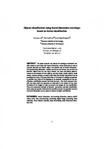
IA = 0, IB↑, IC↑ Two-phase fault of Bgrounded and C IA = 0, IB↑, IC↑ fault of B and C short-circuit fault ofthe the three phases occurred, thevoltage voltage ofeach each phasephase would bereduced. reduced. a short-circuit fault of three the three phases occurred, the voltage of phase each would be reduced. IfIfaaIfshort-circuit fault of phases occurred, the of would be If a single-phase fault occurred, the fault phase current would increase, and the currents of the a single-phase faultoccurred, occurred,the thefault fault phase phase current would increase, and currents of of thethe non-fault If aIf single-phase fault current would increase, andthe the currents If a short-circuit fault decrease. of the three phases occurred, the voltage of each phase would be reduced. non-fault phases would The same class of faults has the same features, and different phases would decrease. class ofoccurred, faults has thevoltage same features, and different of faults non-fault phases would decrease. same class of faults has increase, the samephase features, and different If a short-circuit fault ofThe the same three phases the of each would beclasses reduced. If a single-phase fault occurred, theThe fault phase current would and the currents of the classes of faults have different features [25,26]. The power cable fault state (PCFS) can be denoted by have different features [25,26]. The power cable fault state (PCFS) can be denoted by the sum classes of faults different features [25,26]. Thecurrent power cable fault (PCFS) cancurrents be denoted by of the If a single-phase fault occurred, the fault phase would increase, and the of the non-fault phaseshave would decrease. The same class of faults has thestate same features, and different normal statehave (NS) and decrease. the fault component state (FCS), ashas indicated in(PCFS) Equation (1) and Figure non-fault phases would The[25,26]. same The class of faults thestate same features, and different classes of faults different features power cable fault can be denoted by 1. classes of faults have different features [25,26]. The power cable fault state (PCFS) can be denoted by FCS = PCFS − NS

(1)

Algorithms 2016, 9, 66

3 of 12


3 of 12

the sum of the normal state (NS) and the fault component state (FCS), as indicated in Equation (1) and Figure 1. of the normal state (NS) and the fault component state (FCS), as indicated in Equation (1) the sum and Figure2016, 1. 9, 66 Algorithms

3 of 12(1)

FCS = PCFS − NS FCS = PCFS − NS

(1)

(a) (a)

(b) (b)

(c) (c)

Figure 1. Power cablecable states of (a) fault component state (FCS); fault state (PCFS); (PCFS); Figure Power cable states of component state (FCS); (b)(b) power cablecable fault state and Figure 1.1.Power states of (a) (a)fault fault component state (FCS); (b)power power cable fault(PCFS); state and (c) normal state (NS). (c)(c) normal state (NS). and normal state (NS).

The fault components existexist in the added abnormal voltageof ofthe the The fault components in the added abnormalstate stateofofthe thepower power cable. cable. The voltage The fault components exist in the added abnormal state of the power cable. The voltage of the fault fault components can can be obtained by by thethe differences between fault occurrence occurrence components be obtained differences betweenthe thecable cablevoltage voltage after after fault fault components can be obtained by the differences between the cable voltage after fault occurrence andvoltage the voltage of normal the normal state. Similarly, the currentofofthe thefault faultcomponents components can be obtained by and the of the state. Similarly, the current be obtained by and the voltage of the normal state. Similarly, the current of the fault components can be obtained by thethe differences between the current after fault occurrence and the current of the normal state. the differences between the cable current after fault occurrence and the normal normalstate. state. differences between thecable cable current after fault occurrence andthe thecurrent current of of In a practical system of an online power cable, the n periods of voltage or current before fault In a practical system of anofonline power cable, the voltageororcurrent current before fault In a practical system an online power cable, thennperiods periods of of voltage before fault occurrence are regarded as the voltage or current of the normal state. The voltage or current of occurrence are regarded as the or current ofofthe Thevoltage voltageoror current ofthe the occurrence are regarded as voltage the voltage or current thenormal normal state. state. The current of the fault components S g (t) can be calculated as follows [27]. fault components Sg (t)be can be calculated as follows [27]. fault components Sg(t) can calculated as follows [27]. n

(1−)n11)S −nT nT )n(S St((− tt − nT/2 SgS(Sgt ()gt(=)t )=S=(StS()(t−)t )− (−−(− / 2/ 2) ))

(2) (2) (2)

where S(t) is the voltage or the current after fault occurrence, T is the power frequency period, and

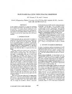
where the voltage or the currentafter afterfault fault occurrence, is the power frequency period,period, and n isand where S(t) is S(t) the isvoltage or the current occurrence,T T is the power frequency n is a positive natural number (usually, n = 2). a positive natural number (usually, n = 2). n is a positive natural number (usually, n = 2). The difference or orcurrent currentdifference differenceof of a period.The The fault Thefault faultcomponent component isis the the voltage voltage difference a period. fault The fault component is the voltage difference or current difference of a period. The fault component should forfault faultrecognition. recognition. component shouldalso alsosatisfy satisfythe the time time requirement requirement for component should also satisfyof the time requirement for recognition. The fault asfault the initial initial signalsofofthe thepower power cable fault The faultcomponent component ofthe thecurrent current was was taken taken as the signals cable fault in in The fault component of the current was taken as the initial of the power this paper. (1) to to obtain obtainthe thefault faultcomponents components of the power cable incable thetypes 10fault types this paper.We Weused usedEquation Equation (1) ofsignals the power cable in the 10 of in this paper. We used Equation (1) to obtain the fault components of the power cable infaults, the 10 types of short-circuit short-circuit states. includes three types of single-phase three types of two-phase faults, states. It It includes three types of single-phase faults,faults, three types of two-phase three of short-circuit states. It grounded includes three oftype single-phase three of two-phase faults, types of two-phase faults, types and one of three-phase faults. Thetypes three phase currents three types of two-phase grounded faults, and one type faults, of three-phase faults. The three and phase their fault components of the single-phase Aand earth faults areAshown infaults Figure 2.faults. The blueThe are2.for threecurrents types ofand two-phase faults, one type ofearth three-phase three phase their faultgrounded components of the single-phase are shown incurves Figure The phase A, the are B, and thefor green curves are the for phase C. blue curves arered forcurves phase A, for thephase redofcurves are phase and green curves arein forFigure phase C. currents and their fault components the single-phase AB,earth faults are shown 2. The blue curves are for phase A, the red curves are for phase B, and the green curves are for phase C. 5

i/A

I/A

Phase A

Phase A Phase B Phase C

50

0

0

-50 0

0.02

0.04

0.06 t/s

0.08

0.1

0.12

-5 0

(a)

0.02

0.04

0.06 t/s

(b) Figure 2. Cont.

0.08

0.1

0.12

Algorithms 2016, 9, 66 Algorithms 2016, 9, 66

4 of 12

4 of 12

5

40

Phase B

Phase C

0

i/A

i/A

20 0 -20 -5 0

0.02

0.04

0.06 t/s

0.08

0.1

-40 0

0.12

0.02

0.04

(c)

0.06 t/s

0.08

0.1

0.12

(d)

Figure 2. (a) Three-phase groundedfault; fault; Fault component of phase Figure 2. (a) Three-phasecurrents currentsof of aa single-phase single-phase AAgrounded (b)(b) Fault component of phase A; A; (c) Fault component of phase B; (d) Fault component of phase C. (c) Fault component of phase B; (d) Fault component of phase C.

3. The Improved Fractal Box Dimension 3. The Improved Fractal Box Dimension(IFBD) (IFBD)Recognition RecognitionAlgorithm Algorithm TheThe fractal dimension can of the the fine finedistributed distributedsignals, signals,and and fractal dimension caneffectively effectivelymeasure measurethe the change change of it it keeps invariant areprocessed processedat at different scales. Particularly, thedimension box dimension keeps invariantififthe the signals signals are different scales. Particularly, the box is more is more suitable for inuse in calculating figure or a sport discrete sport set. the Therefore, the boxwas dimension suitable for use calculating a figurea or a discrete set. Therefore, box dimension chosen this paper as the baseas tothe extract feature [28–30]. wasinchosen in this paper basethe to fault extract the fault feature [28–30]. Definition of the ImprovedFractal FractalBox BoxDimension Dimension 3.1.3.1. Definition of the Improved n

traditional box dimensionDim Dim(S (Sr)r )of ofthe thepoint point set set S Srr in in aa linear linear space TheThe traditional box dimension spaceRRn isis Dim( S(Sr r)) ==lim lim Dim n→∞ n→ ∞

lnN lnN nn((SSr )r ) n ln2 ln2 n

(3) (3)

where n is lengthofofa aside sideof ofaa square square box box which represents the n (S) n(S) represents the where n is thethe length which covers coversthe thepoint pointset setSrS. r.NN minimum number of boxes containing S . minimum number of boxes containing Sr.r By using the above approximation method, the box dimensions of the fault components of phase By using the above approximation method, the box dimensions of the fault components of A, phase B, and phase C are calculated in the condition of the phase A earth fault shown in Figure 1. phase A, phase B, and phase C are calculated in the condition of the phase A earth fault shown in Dim (SA ) = 1.56030, Dim (SB ) = 1.57527, Dim (SC ) = 1.54622. Figure 1. Dim (SA) = 1.56030, Dim (SB) = 1.57527, Dim (SC) = 1.54622. For the curves in a plane, their box dimensions always range from one to two. To make the fault For the curves in a plane, their box dimensions always range from one to two. To make the fault classification easier, we can enlarge the distances between the different classes of the 10 types of the classification can on enlarge the distances between the different of the types of the short circuiteasier, faults.we Based experiments, we defined the improved box classes dimension F as10follows. short circuit faults. Based on experiments, we defined the improved box dimension F as follows. Dim(S) F = tan Dim( S ) (4) F = tan E( Dim∗*) (4)

E ( Dim )

where “tan” represents the tangent function, and E(Dim*) is the expectation of the traditional box where “tan” represents the tangent and state, E(Dim*) the traditional box dimension Dim of the phase currentfunction, in the normal andisit the can expectation be written asof follows.

dimension Dim of the phase current in the normal state, and it can be written as follows. 1

m

1 ∑m Dim (Sr ) E ( Dim ) = m r= 1 Dim ( S r ) m r =1 E( Dim∗ ∗ ) =

(5)

(5)

where Sr is the current signals of the power cable in normal state, r = 1, 2, · · · , m, and m is a positive

where Sr isgreater the current signals of the power cable in normal state, integer than three.

r = 1, 2,L , m , and m is a positive

integer According greater than to three. Equation (4), we have the improved box dimensions FA , FB , and FC of the fault components three phase Accordingoftothe Equation (4), currents. we have the improved box dimensions FA, FB, and FC of the fault components of the three phase currents. Dim(S A ) FA = tan (6) Dim ( S∗A)) E( Dim FA = tan (6) E ( Dim* ) Dim(SB ) FB = tan (7) E( Dim∗ )

FB = tan

Dim( S B ) E ( Dim* )

(7)

E (Dim ) FB = tan

Dim( S B ) E ( Dim* )

(7)


5 of 12

Dim( SC ) Dim SC ) * ) E ((Dim FC = tan ∗ FC = tan

(8) (8)

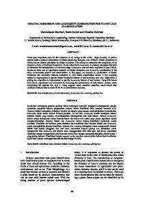
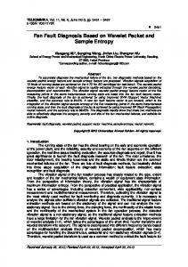
E( Dim ) where Dim(SA), Dim(SB), and Dim(SC) are the traditional box dimensions of the currents of phase A, B, where Dim(SA ), Dim(SB ), and Dim(SC ) are the traditional box dimensions of the currents of phase A, and C, respectively. E(Dim*) is the expectation of the traditional box dimension Dim of the phase B, and C, respectively. E(Dim*) is the expectation of the traditional box dimension Dim of the phase current in the normal state. “tan” represents the tangent function. current in the normal state. “tan” represents the tangent function. For the 10 detailed classes of the short circuit faults, the fault features using the traditional box For the 10 detailed classes of the short circuit faults, the fault features using the traditional box dimension are shown shown in in Figure Figure3a,b 3a and Figure 3bThe respectively. dimensionand andthe theimproved improved box box dimension dimension are respectively. horizontalThe horizontal axis represents the short circuit faults which include the 10 classes of short circuit faults. axis represents the short circuit faults which include the 10 classes of short circuit faults. AG, BG, and AG, andsingle-phase CG are the single-phase short AB, circuit AB, AC are the phase-between short CG BG, are the short circuit faults. BC,faults. and AC areBC, theand phase-between short circuit faults. circuit faults. ABG, BCG, and ACG are the double-phase short circuit faults. ABC is the three-phase ABG, BCG, and ACG are the double-phase short circuit faults. ABC is the three-phase short circuit short fault. The axisfeature is the values. fault feature values. blue color represents phase A, the fault.circuit The vertical axis vertical is the fault The blue colorThe represents phase A, the green color green color represents phase B, and the red color represents phase C. represents phase B, and the red color represents phase C. 7

Fa Fb Fc

6

7

Fa Fb Fc

6

5 5

4

4

3

3

2

2

1 0

1

AG

BG

CG

AB ABG AC ACG BC BCG ABC

0

AG

BG

CG

AB ABG AC ACG BC BCG ABC

(a)

(b)

Figure of the the10 10types typesofofshort shortcircuit circuit faults using traditional Figure3.3.Fault Faultfeature feature histogram histogram of faults byby using (a)(a) thethe traditional boxbox dimension; and (b) the improved box dimension. dimension; and (b) the improved box dimension.

From is clear the traditional box dimension features of theare 10relatively classes are From Figure Figure 3,3,it itis clear thatthat the traditional box dimension features of the 10 classes relatively crowded. to Compared to box the dimension traditionalfeatures, box dimension features, the improved crowded. Compared the traditional the improved box dimension features ofbox dimension features of the 10 classes have larger distances among the single-phase fault and the 10 classes have larger distances among the single-phase fault and the double-phase fault, as well as the double-phase well as thethethree-phase fault. Furthermore, box dimension the three-phasefault, fault.as Furthermore, improved box dimension features the haveimproved larger distances among features havesingle-phase larger distances single-phase faults ofdimension A, B, and feature C. Obviously, the different faultsamong of A, B, the anddifferent C. Obviously, the improved box is better the improved box dimension featureofisthe better for power short circuit faultthe recognition the online power cable for short circuit fault recognition online cable than traditionalof box dimension feature. than the traditional box dimension feature. 3.2. The Improved Fractal Box Dimension (IFBD) Recognition Algorithm

3.2. The ImprovedtoFractal Box Dimension (IFBD) Recognition According the improved box dimension of EquationsAlgorithm (6)–(8), we calculated the improved box dimension features the short circuits. Based on calculation results, we found the According to theofimproved box dimension ofthe Equations (6)–(8), we calculated therelationship improved box between the fault classes and the IFBD features, shown in Table 2 below. We found that the improved dimension features of the short circuits. Based on the calculation results, we found the relationship box dimension features have a similar relationship in the cases of the two-phase grounded faults and between the fault classes and the IFBD features, shown in Table 2 below. We found that the the two-phase-between faults. After the three phase currents or voltages were collected, we could use improved box dimension features have a similar relationship in the cases of the two-phase grounded the relationship to classify the fault.

faults and the two-phase-between faults. After the three phase currents or voltages were collected, we could use the relationship to classify the fault. Table 2. Relationship between the fault classes and the IFBD features. Types of Short Circuit Faults

Feature Relationship

Three-phase faults Single-phase faults Two-phase faults of A and B Two-phase faults of A and C Two-phase faults of B and C

Fc > Fa > Fb Fb > Fa > Fc Fa > Fb > Fc Fa > Fc > Fb Fc > Fb > Fa


6 of 12

The three phase currents were chosen as the original signals of the online power cable. The IFBD recognition algorithm could be described as follows. Step 1: Step 2:

Step 3:

Step 4:

Input the three phase currents. Extract the current signals of any phase in fault state, and calculate the traditional box dimensions Dim(SA ), Dim(SB ), and Dim(SC ) of the fault components of phase A, B, and C using Equation (3). Substitute the traditional box dimensions Dim(SA ), Dim(SB ), and Dim(SC ) respectively into Equations (6)–(8) to calculate the improved box dimension features FA , FB , and FC of the fault components of the three phase currents. Classify the short circuit fault according to Table 2.

4. The Developed Maximum Wavelet Coefficient (DMWC) Recognition Algorithm In this section, we develop the DMWC recognition algorithm for the single-phase grounded faults (DMWCSP) and the two-phase grounded faults (DMWCTP). Similar to the previous IFBD recognition algorithm, the three phase currents were chosen as the original signals of the online power cable for the DMWC recognition algorithm. In the fault state, the three phase components are asymmetric and interlocked, so the calculation and analyses are complex. After the K-transform below, we obtained the α modulus, the β modulus, and the 0 modulus of the three phases.    i0 = iα =   i = β

1 3 1 3 1 3

(i A + i B + iC ) (i A − i B ) (i A − iC )

(9)

where iA , iB , and iC are the three phase currents of the online power cable. The modulus components of 0, β, and α for the different faults are shown in Table 3. It can be seen that the different classes of faults correspond to different patterns of the modulus α, modulus β, and the modulus 0. The DMWC algorithm of DMWCSP and DMWCTP are developed below. Table 3. Modulus components of α, β, and 0 for the different faults. Type of Fault

Boundary Condition

0 Modulus

α Modulus

β Modulus

Grounded fault of phase A Grounded fault of phase B Grounded fault of phase C Phase-between fault of A and B Phase-between fault of A and C Phase-between fault of B and C Grounded faults of A and B Grounded faults of A and C Grounded faults of B and C Grounded fault of A, B, and C

ib = ic = 0 i a = ic = 0 i a = ib = 0 i a + ib = 0, ic = 0 i a + ic = 0, ib = 0 ic + ib = 0, i a = 0 ic = 0 ib = 0 ia = 0 i a + ib + ic = 0

ia ib ic 0 0 0 i a + ib i a + ic ib + ic 0

ia −ib 0 2i a −ib ia i a − ib ia −ib i a − ib

ia 0 −ic ia ib 2i a ia i a − ic −ic i a − ic

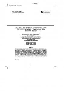
Based on the experiments, the wavelet Db3 were used to analyze the modulus components of α, β, and 0 for the different faults. The maximum wavelet coefficients I0 , Iα , and Iβ are listed in Table 4 for the 10 types of short circuit faults. The flow chart of the calculation of the maximum wavelet coefficients [31] is shown in Figure 4.

for the 10 types of short circuit faults. The flow chart of the calculation of the maximum wavelet coefficients [31] is shown in Figure 4. Table 4. Maximum wavelet coefficients I0, Iα, and Iβ of the different faults. Algorithms 2016, 9, 66

Fault

I0

Iα

Iβ

Grounded fault of A

0.2997

0.2997

0.2997

Table 4.fault Maximum I0 , Iα , and Iβ of the4.5535 different faults. Grounded of B wavelet coefficients 4.5535

0.0003

Grounded fault of C

4.8586

Fault

Phase-between fault of A and B

Grounded fault of A GroundedGrounded faults offault A and of BB Grounded C C Phase-between fault fault of A of and Phase-between fault of A and B Grounded faultsfaults of Aofand C B Grounded A and Phase-between A and Phase-between faultfault of Bofand CC Grounded faults of A and C Grounded faults offault B and Phase-between of B C and C Grounded faults of and B andCC Grounded fault of A, B, Grounded fault of A, B, and C

4.8586 I0

0.0000

0.2997 4.5173 4.5535 4.8586 0.0000 0.0000 4.2387 4.5173 0.0000 0.0001 4.2387 0.2786 0.0001 0.2786 0.0000 0.0000

Iα

0.0001 4.6010

0.2997 4.6010 4.5535 0.0001 2.7855 4.6010 2.0056 4.6010 2.7855 5.0865 2.0056 4.9471 5.0865 4.9471 4.6010 4.6010

Iβ 0.2997 0.0003 4.8586 2.3005 1.8867 5.5721 5.5721 5.0865 5.2260 5.5721

7 of 12

2.3005 1.8867 5.5721 5.5721 5.0865 5.2260 5.5721

Figure4.4.Flow Flowchart chartofofthe thecalculation calculation of of the the maximum Figure maximumwavelet waveletcoefficients. coefficients.

The proposedDMWCSP DMWCSPalgorithm algorithm is is described described below. The proposed below.

Step 1: 1:Calculate the the modulus components phasecurrents currentsiAi,Ai,B i,Band , and C by Step Calculate modulus componentsi0,i0i,αi,αand , andiβiβof ofthe the three three phase iC iby using the K-transform. using the K-transform. Step 2: 2: Calculate the maximum wavelet coefficients Iα Iand Iβ Iof the modulus Calculate the maximum wavelet coefficients the moduluscomponents componentsiiααand and iiββby Step α and β of using the Wavelet transform. by using the Wavelet transform. Step 3: If fault is classified as the grounded fault of C.fault Otherwise, go to the next step. Iα FC , classify the as the phase-between if Ior 0.01 as the Step 5: 5: If FA If> FFBA>>FCF,Bclassify the fault asfault the phase-between fault offault AB ifofI0 AB < 0.01 theor two-phase 0 0.01. go to the next step. grounded fault ofgrounded AB if I0 > fault 0.01. of Otherwise, go toOtherwise, the next step. Step > FB , classify the as the phase-between if Ior 0.01 as the Step 6: 6: If FA If> FFCA>>FBF,Cclassify the fault asfault the phase-between fault offault AC ifofI0 AC < 0.01 theor two-phase 0 0.01. go to the next step. grounded fault ofgrounded AC if I0 >fault 0.01.of Otherwise, go toOtherwise, the next step. Step > FA , classify the as the phase-between if Ior 0.01 as the Step 7: 7: If FC If > FFBC>>FAF,Bclassify the fault asfault the phase-between fault offault BC ifofI0 BC < 0.01 theor two-phase 0 0.01. Otherwise, go to the next step. grounded fault of BC if I0 > 0.01. Otherwise, go to the next step. 0 Step FC , classify fault single-phasegrounded grounded fault of asas thethe Step 8: 8:If FBIf>FFBA>>FFAC,>classify the the fault as as thethe single-phase of CCififIαIα β0.01. Otherwise, classify the fault as the single-phase grounded grounded fault offault A. of A.

Figure5.5.Flow Flowchart chart of of the the fusion fusion sensing Figure sensing(FS) (FS)method. method.

6. Experiment and Results 6.1. Experimental Environment The experimental system structure is shown in Figure 6.

The experimental system structure is shown in Figure 6. The LabVIEW software was used for the interface platform. The diameter of the power cable was 2.5 mm. The power supply was the three phase variable-frequency power SPS-HL-3300 N, which changed the voltage from 380 V to 90 V.


9 of 12

Figure 6. Experimental system structure.

Figure 6. Experimental system structure.

The LabVIEW software was used for the interface platform. The diameter of the power cable The starThe connection mode was withphase the neutrals grounded. The signal collection N, card was was 2.5 mm. power supply was used the three variable-frequency power SPS-HL-3300 which achanged NI PCI-9203. The closed-loop Hoare current sensors CHB-25NP were from Beijing SENSOR the voltage from 380 V to 90 V. Electronics Co., Ltd. (Beijing, The star connection modeChina). was used with the neutrals grounded. The signal collection card was a NI PCI-9203. The closed-loop Hoare current sensors CHB-25NP were from Beijing SENSOR Electronics 6.2. Experiment Results and Analysis Co., Ltd. (Beijing, China). Table 5 shows the IFBD recognition process and the results with an initial angle of 30° and a 6.2. Experiment Analysis fault resistance Results of 30 Ω.and Table 6 shows the DMWC recognition process and the results with the initial angleTable of 30°5 shows and fault resistances of 30 Ωprocess and 300and Ω. the results with an initial angle of 30◦ and a fault the IFBD recognition resistance of 30 Ω. Table 6 shows the DMWC recognition process and the results with the initial angle 5. IFBDof recognition of 30◦ and faultTable resistances 30 Ω andwith 300 initial Ω. angle of 30° and fault resistance of 30 Ω. Dim(SA) Dim(SB) Dim(SC) FA FB FC Recognition Result ◦ and fault resistance of 30 Ω. Table 5. IFBD with initial angle of 305.79713 1.56129 1.58036 1.54921recognition 6.20045 6.96163 Single-phase grounded fault 1.55953 1.58077 1.54182 6.13833 6.98000 5.57463 Single-phase grounded fault Dim(SA ) 1.58127 Dim(SB ) 1.54840 Dim(SC ) 6.26345 FA FB FC Recognition Result fault 1.56304 7.00254 5.77191 Single-phase grounded 1.47034 1.43155 1.20976 4.04967 3.51537 1.93227 Phase-between fault offault AB 1.56129 1.58036 1.54921 6.20045 6.96163 5.79713 Single-phase grounded 1.47022 3.61930 1.98314 Two-phase grounded fault of AB 1.55953 1.43993 1.58077 1.22141 1.54182 4.04778 6.13833 6.98000 5.57463 Single-phase grounded fault 1.47985 1.97674 3.66650 Phase-between fault offault AC 1.56304 1.21997 1.58127 1.44359 1.54840 4.20460 6.26345 7.00254 5.77191 Single-phase grounded 1.47701 1.97838 3.72746 Two-phase grounded of AC 1.47034 1.22034 1.43155 1.44819 1.20976 4.15717 4.04967 3.51537 1.93227 Phase-between faultfault of AB 1.47022 1.43805 1.43993 1.47034 1.22141 1.34675 4.04778 3.61930 1.98314 Two-phase grounded fault 1.03145 3.59549 4.04967 Phase-between fault of of BCAB 1.47985 1.43032 1.21997 1.46975 1.44359 1.41522 4.20460 1.97674 3.66650 Phase-between faultfault of AC 1.05752 3.50058 4.04041 Two-phase grounded of BC 1.47701 1.12408 1.22034 1.19392 1.44819 1.73838 4.15717 1.97838 3.72746 Two-phase 1.16057 1.61290 1.86633 Three-phasegrounded groundedfault faultof ofAC ABC 1.03145 1.43805 1.47034 1.34675 3.59549 4.04967 Phase-between fault of BC 1.05752 1.43032 1.46975 1.41522 3.50058 4.04041 Two-phase grounded fault of BC 6. DMWC recognition with different 1.16057 1.12408 Table 1.19392 1.73838 1.61290 1.86633fault resistances. Three-phase grounded fault of ABC

Initial Fault I0 Recognition Result Iβ Iα Table 6. DMWC recognition with different fault resistances. Angle Resistance 30° 30 Ω 5.3462 5.3462 5.3462 Single-phase grounded fault of A Iβ Initial Angle Fault Resistance I Iα Recognition Result 30° 30 Ω 11.8208 0 11.8208 0.0015 Single-phase grounded fault of B ◦ 30 30 Ω 5.3462 5.3462 5.3462 Single-phase grounded fault of A 30° 30 Ω 30 Ω 6.4669 11.8208 0.0105 11.8208 6.4746 0.0015 Single-phase grounded fault of C 30◦ Single-phase grounded fault of B ◦ 30° 30 Ω 30 Ω 0 20.4730 0.0105 10.2362 6.4746 Phase-between fault offault AB of C 30 6.4669 Single-phase grounded 30◦ 30 Ω 0 0.6722 20.4730 10.2362 Phase-between Phase-between fault of AB 30° 30 Ω 0 1.3458 fault of AC ◦ 30 30◦ 30◦ 30◦ 30◦ 30◦ 30◦ 30◦

30 Ω 30 Ω 300 Ω 300 Ω 300 Ω 300 Ω 300 Ω 300 Ω

0 0 0.8570 1.8927 1.0367 0 0 0

0.6722 10.9097 0.8571 1.8927 0.0105 2.8251 0.0922 1.5057

1.3458 10.9091 0.8570 0.0015 1.0379 1.4122 0.1857 1.5051

Phase-between fault of AC Phase-between fault of BC Single-phase grounded fault of A Single-phase grounded fault of B Single-phase grounded fault of C Phase-between fault of AB Phase-between fault of AC Phase-between fault of BC


10 of 12

Table 7 shows the comparison of the DMWC recognition method and the FS method with different initial angles 0◦ , 30◦ , and 90◦ , and fault resistances of 30 Ω, 150 Ω, and 300 Ω. Table 8 shows the comparison of the DMWC recognition method and the FS method with different initial angles of 0◦ and 30◦ , and different fault distances of 0.8 km, 8 km, and 30 km. Table 7. Comparison of DMWC and FS with different fault resistances. Initial Angle 0◦

0◦ 30◦ 30◦ 90◦ 90◦ 90◦

Fault Resistance

30 Ω 150 Ω 30 Ω 150 Ω 30 Ω 150 Ω 300 Ω Mean value

Recognition by DMWC

Recognition by FS

91% 86% 88% 79% 75% 72% 71% 80.3%

97% 96% 95% 93% 98% 98% 97% 96.3%

Table 8. Comparison of DMWC and FS with different fault distances. Initial Angle 0◦

0◦ 0◦ 90◦ 90◦ 90◦

Fault Distance

0.8 km 8 km 30 km 0.8 km 8 km 30 km Mean value

Recognition Results by DMWC

Recognition Results by FS

96% 95% 92% 85% 81% 78% 87.8%

99% 99% 98% 98% 97% 97% 98.0%

It can be seen from Table 5 that the IFBD recognition algorithm could classify 8 of the 10 types of short circuit faults. It could recognize the single-phase grounded faults, but could distinguish the detailed fault phase of A, B, or C. The experiments proved that the DMWC recognition algorithm could correctly classify all 10 types of short circuit faults. In addition, the fault resistances had no influence on the recognition result of the DMWC recognition algorithm. Therefore, this algorithm is better than the IFBD recognition algorithm regarding fault type recognition. It can be seen from Tables 7 and 8 that the FS method could correctly classify all 10 types of short circuit faults. The initial angle, the fault resistance, and the fault distance had no influence on the recognition result of the FS method. Therefore, the FS method is better than the IFBD recognition algorithm and the DMWC recognition algorithm regarding their comprehensive performances. 7. Conclusions The IFBD algorithm was developed to enlarge the distances between 10 classes of short circuit faults by using the improved fractal dimension feature extracted from the three-phase currents for the first stage of fault recognition. K-transform and wavelet analysis were then used to establish the relationship between the modulus value and the fault class, and the DMWC recognition algorithm was developed. The IFBD algorithm and the DMWC algorithm were then combined to produce the FS method. Finally, the test system was utilized with the LabVIEW platform. The FS method was experimentally proven to effectively recognize all 10 classes of short circuit faults. The FS method was also not influenced by the parameters of the initial angle, transient resistance, and the fault distance. Compared with the DMWC algorithm, the FS method improved the recognition accuracy from 80.3% to 96.3% in the case of varied fault resistances, and improved the recognition accuracy from 87.8% to 98.0% in the case of varied fault distances.


11 of 12

Acknowledgments: This research was sponsored by the Natural Science Foundation of China (51405381), the Key Scientific and Technological Project of Shaanxi Province (2016GY-040), and the Science Foundation of Xi’an University of Science and Technology (104-6319900001). Author Contributions: M.W. conceived and designed the experiments; L.Z. and Y.G. performed the experiments; M.W. and L.Z. and Y.G. analyzed the data; M.W. and L.Z. and Y.G. wrote the paper. Conflicts of Interest: The authors declare no conflict of interest.

References 1. 2. 3. 4. 5. 6.

7. 8. 9. 10. 11. 12. 13. 14. 15. 16. 17. 18.

19.

20.

Zhao, J.H.; Xu, Y.; Luo, F.J.; Dong, Z.Y.; Peng, Y.Y. Power system fault diagnosis based on history driven differential evolution and stochastic time domain simulation. Inf. Sci. 2014, 275, 13–14. [CrossRef] Prasad, A.; Edward, J.B. Application of Wavelet Technique for Fault Classification in Transmission. Procedia Comput. Sci. 2016, 92, 78–81. [CrossRef] Jun, J.T.; Feng, P.F.; Wei, S.L.; Zhang, H.; Liu, Y.F. Investigation on the surface morphology of Si3 N4 ceramics by a new fractal dimension calculation method. Appl. Surf. Sci. 2016, 387, 813–817. Guclu, S.O.; Ozcelebi, T.; Lukkien, J. Distributed Fault Detection in Smart Spaces Based on Trust Management. Procedia Comput. Sci. 2016, 83, 66–70. [CrossRef] Bharata, M.J.; Gopakumar, P.; Mohanta, D.K. A novel transmission line protection using DOST and SVM. Eng. Sci. Technol. 2016, 19, 1027–1037. Lin, S.; Mei, J.T.; Chen, S.; He, Z.Y.; Qian, Q.Q. Fault Detection and Faulty Phase Determination of Transmission Lines Based on Time-Frequency Characteristics of Transient Travelling Waves. Power Syst. Technol. 2012, 36, 49–52. Chicharro, F.I.; Cordero, A.; Torregrosa, J.R. Dynamics and Fractal Dimension of Steffensen-Type Methods. Algorithms 2015, 8, 271–279. [CrossRef] Gómez, M.J.; Castejón, C.; García-Prada, J.C. Review of Recent Advances in the Application of the Wavelet Transform to Diagnose Cracked Rotors. Algorithms 2016, 9, 19. [CrossRef] Zhou, W.; Xiong, J.; Li, F.; Jiang, N.; Zhao, N. Fusion of Multiple Pyroelectric Characteristics for Human Body Identification. Algorithms 2014, 7, 685–702. [CrossRef] Tan, X.H.; Liu, J.Y.; Li, X.P.; Zhang, L.H.; Cai, J.C. A simulation method for permeability of porous media based on multiple fractal model. Int. J. Eng. Sci. 2015, 95, 76–80. [CrossRef] Yu, M.Z.; Chan, T.L. A bimodal moment method model for submicron fractal-like agglomerates undergoing Brownian coagulation. J. Aerosol Sci. 2015, 88, 25–30. [CrossRef] Martino, G.D.; Iodice, A.; Riccio, D.; Ruello, G.; Zinno, I. Angle Independence Properties of Fractal Dimension Maps Estimated From SAR Data. IEEE J. Sel. Top. Appl. Earth Obs. Remote Sens. 2013, 6, 1242–1248. [CrossRef] Nelson, J.D.B.; Kingsbury, N.G. Fractal dimension, wavelet shrinkage and anomaly detection for mine hunting. IET Signal Process. 2012, 6, 485–487. [CrossRef] Reza, F.M.; Qi, X.J. Face Recognition under Varying Illumination with Logarithmic Fractal Analysis. IEEE Signal Process. Lett. 2014, 21, 1459–1460. Xu, Y.; Liu, D.L.; Quan, Y.H.; Callet, P.L. Fractal Analysis for Reduced Reference Image Quality Assessment. IEEE Trans. Image Process. 2015, 24, 2099–2100. [CrossRef] [PubMed] Tumu, I.; Concas, G.; Marchesi, M.; Tonelli, R. The fractal dimension of software networks as a global quality metric. Inf. Sci. 2013, 245, 295–299. Liu, J.H.; Liang, R.; Wang, C.L.; Fan, D.P. Application of fractal theory in detecting low current faults of power distribution system in coal mines. Min Sci. Technol. (China) 2009, 19, 321–323. [CrossRef] Usama, Y.; Liu, X.M.; Imam, H.; Sen, C.; Kar, N.C. Design and implementation of a wavelet analysis-based shunt fault detection and identification module for transmission lines application. IET Gener. Transm. Distrib. 2014, 8, 431–440. [CrossRef] Zhang, S.W.; Zhang, F.; Wang, Z.J.; Gu, H.Y.; Ning, Q. Series Arc Fault Identification Method Based on Energy Produced by Wavelet Transformation and Neural Network. Trans. China Electrotech. Soc. 2014, 29, 291–293. Gopakumar, P.; Reddy, M.J.B.; Mohanta, D.K. Transmission line fault detection and localisation methodology using PMU measurements. IET Gener. Transm. Distrib. 2015, 9, 1033–1039. [CrossRef]


21. 22. 23. 24. 25. 26.

27.

28. 29. 30. 31.

12 of 12

Zhang, L.L.; Xu, B.Y.; Xue, Y.D.; Gao, H.L. Transient Fault Locating Method Based on Line Voltage and Zero-mode Current in Non-solidly Earthed Network. Proc. CSEE 2012, 32, 110–113. Prasad, A.; Edward, J.B. Application of Wavelet Technique for Fault Classification in Transmission Systems. Procedia Comput. Sci. 2016, 92, 78–83. [CrossRef] Dai, H.Z.; Zheng, Z.B.; Wang, W. A new fractional wavelet transform. Commun. Nonlinear Sci. Numer. Simul. 2017, 44, 19–32. [CrossRef] Wu, Q.; Law, R. Complex system fault diagnosis based on a fuzzy robust wavelet support vector classifier and an adaptive Gaussian particle swarm optimization. Inf. Sci. 2010, 180, 4515–4520. [CrossRef] Zheng, G.P.; Zhang, L.; Jiang, C.; Qi, Z.; Yang, Y.H. Line and Segment Online Location of Single-phase-to-earth Fault in the Ungrounded Neutral System. Autom. Electr. Power Syst. 2013, 37, 111–113. Jiang, J.A.; Chuang, C.L.; Wang, Y.C.; Hung, C.H.; Wang, J.Y.; Lee, C.H.; Hsiao, Y.T. A Hybrid Framework for Fault Detection, Classification, and Location—Part I: Concept, Structure, and Methodology. IEEE Trans. Power Deliv. 2011, 26, 1990–1998. [CrossRef] Tang, G.; Hou, W.; Wang, H.Q.; Luo, G.G.; Ma, J.W. Compressive Sensing of Roller Bearing Faults via Harmonic Detection from Under-Sampled Vibration Signals. Sensors 2015, 15, 25648–25660. [CrossRef] [PubMed] Wook, K.J.; Kim, J.H.; Seo, J. Multiple Leader Candidate and Competitive Position Allocation for Robust Formation against Member Robot Faults. Sensors 2015, 15, 10777–10780. Han, C.; Zhang, H.Y.; Guo, C.X.; Jiang, C.; Sang, N.; Zhang, L.P. A Remote Sensing Fusion Method Based on the Analysis Sparse Model. IEEE J. Sel. Top. Appl. Earth Obs. Remote Sens. 2016, 9, 1302–1308. [CrossRef] Xu, J.D.; Yu, X.C.; Pei, W.J.; Hu, D.; Zhang, L.B. A remote sensing fusion method based on feedback sparse component analysis. Comput. Geosci. 2015, 85, 116–118. [CrossRef] Cheng, J.; Liu, H.J.; Liu, T.; Wang, F.; Li, H.S. Remote sensing image fusion via wavelet transform and sparse representation. ISPRS J. Photogramm. Remote Sens. 2015, 104, 160–170. [CrossRef] © 2016 by the authors; licensee MDPI, Basel, Switzerland. This article is an open access article distributed under the terms and conditions of the Creative Commons Attribution (CC-BY) license (http://creativecommons.org/licenses/by/4.0/).