Applied Mathematics, 2014, 5, 1733-1740 Published Online June 2014 in SciRes. http://www.scirp.org/journal/am http://dx.doi.org/10.4236/am.2014.512166
Computation of Local Fractal Dimension Values of the Human Cerebral Cortex Richard D. King Center for Alzheimer’s Care, Imaging and Research, Department of Neurology, University of Utah, Salt Lake City, USA Email:
[email protected] Received 25 April 2014; revised 26 May 2014; accepted 4 June 2014 Copyright © 2014 by author and Scientific Research Publishing Inc. This work is licensed under the Creative Commons Attribution International License (CC BY). http://creativecommons.org/licenses/by/4.0/
Abstract Objectives: The purpose of this paper is to describe a technique for computing the local fractal dimension of the human cerebral cortex as extracted from high-resolution magnetic resonance imaging scans. Methods: 3D models of the human cerebral cortex were extracted from high resolution magnetic resonance images of 10 healthy adult volunteers using FreeSurfer. The local fractal dimension of the cortex was computed using a custom-written cube-counting algorithm. The effect of constraining the maximum region size on the measured value of local fractal dimension was examined. A proof of principle was demonstrated by comparing an individual with Alzheimer’s disease to a healthy individual. Results: Local values of cortical fractal dimension can be obtained by constraining the size of the region over which the cube counting is performed. Cubic regions of intermediate size (30 × 30 × 30 mm) yielded a profile that demonstrated greater regional variability compared to smaller (15 × 15 × 15 mm) or larger (60 × 60 × 60 mm) region sizes. Conclusions: Local fractal dimension of the cerebral cortex is a novel measure that may yield additional, quantitative insight into the clinical meaning of cortical shape changes.
Keywords Fractal, Dimension, Cortex, Imaging Biomarkers, Local
1. Introduction Fractal dimension analysis was first made popular by a series of works by Benoit Mandelbrot in the late 1970s and early 1980s [1] [2]. Mathematically created fractal objects, such as Cantor dust or the Sierpinski gasket, exhibit a property called “self-similarity”, which means that magnification of smaller scale features exactly duplicates a larger scale structure. In nature, many objects such as plants (ferns, cauliflower), clouds, mountains, and rivers also exhibit a property of statistical self-similarity. While mathematical objects have an infinite range to How to cite this paper: King, R.D. (2014) Computation of Local Fractal Dimension Values of the Human Cerebral Cortex. Applied Mathematics, 5, 1733-1740. http://dx.doi.org/10.4236/am.2014.512166
R. D. King
their self-similarity, biological objects only exhibit this property over a limited spatial range. The analytic techniques using this principle can model very complicated structures using relatively simple computational algorithms. Fractal analysis has been applied to many fields of natural science including botany, geology, and medicine, to name a few. One particular application that has been advanced in the past decade is the use of fractal dimension as a measure of the complexity of the human cerebral cortex. Studies using anatomical data from either tissue specimens or magnetic resonance images have demonstrated that the human cerebral cortex exhibits fractal properties which arise secondary to cerebral folding [3]-[8]. Fractal analysis has been used to study several neurological conditions, including schizophrenia [9]-[12], multi-systems atrophy [13], epilepsy [14], stroke [15], cortical development [16] [17], and Alzheimer’s disease [18] [19]. When applied to the cerebral cortex, the information obtained by the analysis of fractal dimension is related to, but different from, information obtained using standard volumetric approaches (such as measures of brain volume, surface area, cortical thickness, or gyrification index). Fractal analysis measures integrate information over a range of spatial scales (two orders of magnitude from 0.5 mm to ~30 mm). This unique approach to shaping analysis can integrate several aspects of structural change associated with disease (i.e. both subtle changes in cortical thickness associated with synaptic and neuronal loss as well as larger scale changes in the width and depth of sulci). Most studies of the fractal properties of the cerebral cortex have focused on computing whole-brain measures (i.e. generating one number which summarizes the entire hemisphere). While quantification of whole-brain complexity is useful, it is well established that the brain is not uniformly affected by either aging or by progressive neurodegenerative diseases such as Alzheimer’s disease [20]-[22]. Consequently, performing a local (or regional) analysis may allow for more specific and sensitive cortical complexity changes to be identified that represent the structural influence of non-uniformly distributed cerebral pathology. The purpose of this paper is to describe a technique for computing the local fractal dimension of the human cerebral cortex as extracted from high-resolution magnetic resonance imaging scans. Having a measure of local fractal dimension could serve a number of very useful clinical purposes. First, the measure would provide a reliable quantification to the otherwise subjective and qualitative assessment of cortical shape. Currently used terms for assessing the integrity of the cerebral cortex, such as “mild age-appropriate atrophy”, can be augmented with a quantitative, statistically based measure. Furthermore, the local fractal dimension measure is ideal for identifying subtle changes in brain shape that could be difficult to identify visually. Finally, subtle changes in brain complexity may herald the onset of neurological disease. As such, using the fractal analysis technique to identify structural changes in cortical complexity has potential for clinical use as a neuroimaging biomarker.
2. Methods 2.1. Source Data The raw data used in this study were extracted from high-resolution, high-contrast magnetic resonance images (MP-RAGE sequence, resolution of 1 × 1 × 1.25 mm, TR = 9.7 ms, TE = 4 ms, flip angle = 10 degrees, T1 = 20 ms, and TD = 200 ms). The images were obtained from the clinical database of magnetic resonance images at the University of Utah. All images were de-identified according to Institutional Review Board protocol. For the analysis of region size, 10 age-matched healthy adult subjects were selected. For demonstration of the potential clinical application, one healthy adult subject and one subject with clinically diagnosed Alzheimer’s disease were selected.
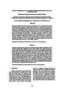
2.2. Image Pre-Processing In brief, we generate three-dimensional models of the cerebral cortex from high-contrast magnetic resonance images using a well-accepted image segmentation program called FreeSurfer. The methods for model generation have been well documented in other publications [23]-[27]. After the original images undergo motion correction and intensity normalization, the extracerebral voxels (or 3D pixels) are removed using a “skull-stripping” procedure. The 3D surfaces are generated based on the intensity values and geometric structure of the cortex (Figure 1(A)). The resulting surface has sub-millimeter accuracy [23] [25]. Each 3D surface is composed of tessellated triangles (~200,000 per hemisphere).
1734
R. D. King
Figure 1. Image pre-processing. 3D models of the cortical surface were generated from high-contrast magnetic resonance images (MP-RAGE sequence) using the FreeSurfer pipeline. A. Original image (in coronal orientation); B. Skull-stripped image with neck removed and intensities normalized; C. 2D projection of the pial and grey/white surface; D. 3D view of the right hemisphere pial surface with a zoom-in on the frontal lobe to illustrate the triangular mesh.
2.3. Computing Local Fractal Dimension Using Cube Counting The 3D Fractal Dimension (f3D) of the cortical surfaces is computed using a 3D cube-counting algorithm. This algorithm has been found to be a robust and accurate method of computing cortical complexity [6] [8] [14] [18] [19] [28]-[31]. This approach is derived from the Minkowski-Bouligand dimension with an extrapolation using 3D cubes instead of 2D boxes. Note that f3D is a unit-less measure. Initially, the 3D surface is tiled with cubes of a uniform size. The cube size is then changed, and the intersection computation is repeated. f3D is computed as the change in the log of the cube count divided by the change in the log of the cube size. See Equation (1). f3 D = −
∆ log ( cube count ) ∆ log ( cube size )
(1)
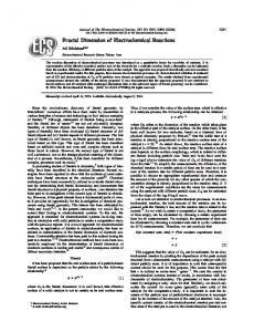
The range of cube sizes depends upon the resolution of the original data (1 mm for the images used in this paper) and the upper size limit of the object to be measured. The human brain is around 150 mm long. The brain has self-similar fractal properties over a limited scale, which for this paper ranged 0.5 mm to 30 mm [19]. The best fit of any tiling could be established by repeating the tiling calculation multiple times with a slight random jitter of the relative position of the tiling cubes to the tessellated mesh. Cube counting in this implementation requires the user to compute the intersection between a tiling grid of fractal counting cubes and the tessellated triangular mesh of the cortical surface. An algorithm for performing an intersection computation between one side of a counting cube and one side of an individual triangular mesh element is shown in Figure 2. This process would need to be repeated for each side of the mesh element and each side of the cube to determine successful intersection or not. Each intersecting box should be identified only once. The entire algorithm for computing the local fractal dimension of a cortical surface model is shown in the flowchart in Figure 3. Note that the process in Figure 2 is contained in a single box in the bottom right corner of Figure 3. The resolution of the final image depends upon the number of center points used to compute the local fractal dimension. For the purpose of this project, it was reasonable to create an image at the same resolution as the original MR image. Every voxel that was labeled as belonging to the cerebral cortex during the image segmentation process described above was used as a center point for this analysis. This generates approximately 600,000 data points per hemisphere.
1735
R. D. King Compute the intersection of a cube and a face
Select one side of cube
Select one line segment (ray) from face edge
Find point of intersection of ray and plane
Cube and face intersect
Save point
Yes No
more rays?
point inside face?
Yes
Side and face intersect
No Cube and face do not intersect 2 points outside face? Yes
No
Yes
Create lines from points
2 lines found?
Yes
No
Yes
Lines intersect? No
No
Side and face do not intersect
more sides?
Figure 2. Flowchart for computing the intersection of side (edge of a triangular mesh element) with a face of a cube. The intersection is identified using standard geometry. Possible intersections for each triangular mesh side (3 edges) and each cube face (6 faces) are computed. 2 Define Region Size
Define Region Center
1 Load Surfaces
Select cube size
Select face
Yes
Yes
Yes No
More center points?
More cube sizes?
More cubes?
No
No 5
2 Local Region
4
Save Total Cube Count
3 Global Tiling
Unique Intersection? Yes
3
Compute regression of box count / box size for each point
1 R. hemisphere
Yes No
More faces?
No
Compute intersection of cube and face
Select Cube
Increment Cube Count
4 Local Tiling
5 Local fractal dimension
2.50
2.90
Figure 3. Flowchart for computing the local fractal dimension of the cerebral cortical surface. The flowchart for the cube-edge algorithm is shown in Figure 2. An example of a complete local fractal dimension computation is shown on the bottom left with local fractal values color-coded using the “heat” color scale.
2.4. Determining the Effect of Region Size The size of the region to be analyzed will likely have a significant effect on the calculated regional variability. If the region size is very large (>0.5 the size of the whole brain), then the regional variation will be averaged across a large swath of cortex, and local values will converge to global values. If the region size is very small (3.0 or