objective is to design a nominal tracking control where out- puts are required to track reference inputs. Februvry 2000. IEEE Control Systems Magarlne. 35 ...
By Hassan Noura, Dominique Sauter, Fr6dBric Hamelin, and Didier Theilliol
auIt- ~ ~ ~ e ~ a n t
JApplication to a Winding Machine
ver the past two decades. the growing demand for reliability in industrial processes has drawn increasing attention to the problem of fault detection and isolation (FDI), but only a lew studies have been dedicated t o t h e related fault-tolerant control (FTC) problem. A fault (abrupt or incipient) is any kind of malfunction o r degradation in the plant that can lead to a reduction in performance or loss of Important functions,impairing safety. Therefore, FTC can be motivated by different goals depending on the application under consideration; for instance, safety in flight control or reliability, or quality improvements in industrial processes. Although FK Is a recent research topic in control theory, the idea of controlling a system that deviates from its nominal operatingconditions has been investlgated by many researchers, The methods for dealing with this problem usually stem from linear-quadratic, adaptive, or robust control. The problems to consider in the design of a fault-tolerant controller are quite particuiar. First, the number of possible faults, and consequently
actions, isverylarge. Second, theoccurrence of afault can make the system evolve far from its normal operating conditions and can lead to a drastic change in system behavior. It is often a rapid change, a n d t h e time for accommodation is veryshort. Furthermore, correct isolation of the faulty component is required to react successfully, a rather difficult problem in the case of closed-loop systems. Finally, FTC is a multivariable problem, with strong coupling between the different variables. Various approaches lor fault-tolerant control have been suggested in the literature [40]. From the applica-
-.
znnn
, /
,,//
tion viewpoint, flight-control systems have represented the main area of research, and only a few studies have been devoted to industrial processes. One of the main goals of this article is to show that these approaches are appropriate to such systems. Fault-tolerant control systems are characterized here by their capabilities, alter fault occurrence, to recover
33
It/ I
Performance
/
Normal Operating Conditions
/
I
I i
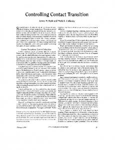
Figure 1. Thejculr-tolerant control problem. performance close to the nominal desired performance. In addition, their ability to react successfully(stably) during a transient period between the fault occurrence and the performance recovery is an important feature. Accommodation capability of acontrol system depends on many factors such a s t he severity of the failure, the robustness of the nominal system, and the actuators' redundancy. Actually, fault-tolerant control concepts can be separated into "passive" and "active" approaches. The passive approach uses robust control techniques to ensure that a closed-loop system remains insensitive to certain faults. When redundant actuators are available, methods dealing with this approach are also called reliable control methods [ X I , [48], [56]. In the active approach, a new set of control parameters is determined such that the faulty system reaches t he nominal system performance. The principle of active approaches, illustrated by Fig. 1, is very simple. After t he fault Occurrence, the system deviates from its nominal operating point defined by its inputjoutput variables (u0,yo) to a faulty one (U, ,y,). The goal ol fault-tolerant control is to determine a new control law that takes the degraded system parameters into account and drives the system to a new operatingpoint(u,,y,)such that themain performance parameters (stability, accuracy, etc.) are preserved (i,e,, are a s close as possible to the initial parameters). It is, therefore. important t o define precisely the degraded modes that are acceptable with regard to the required performance parameters, since alter the occurrence of faults, conventional feedbackcontrol design may result in unsatislactory performance such a s tracking error, instability, and so on. When t he exact model of the failed system is known, the control system can be accommodated so that system performance parameters are recovered and the new system behaves as initially specified. Gao and Antsaklis [ 171, [18] and Morse and Ossman [31] suggest a basic approach based on what theycall the pseudo-inverse method. In practice, however, the faults are unanticipated and the model of the impaired system is not available. To overcome the limitations of conventional feedback control, new controllers have been developed with accom-
34
modation capabilities o r tolerance t o faults. T h e s e fault-tolerant controllers belong to different categories: Adaptive control seems to be the most natural approach to accommodate faults; the faults' effects appear as model parameter changes and are identified online, and the control law is reconfigiired automatically based on new parameters [8], [%I, [42], [55]. Wu et al. [54] consider a loss of effectiveness in actuators ancl suggest using an augmented state Kalman filter to estimate both the fault-free state and the faulty parameters. The estimated fault-tree state is used to feed the controller. All these approaches have theadvantage of not requiringthat thelaults be categorized a priori, although the design of robust identification and control algorithms presents significant challenges. Integrated approaches represent another tread [33]. They integrate fault monitoring and control procedures. In this case, the possible actuator or sensor faults are represented by signals and are estimated by the same algorithm that computes the control law [32], [44], [47]. The faults are modeled first, then the controller is built to be insensitive to these faults, but the operator should be aware of possible faults through the alarm-monitoring function. * The fault-tolerant control problem can also be formulated as a multiobjective problem based on the assumption that, like the uncertainties, the faults' effects can be expressed by means of linear fractional transformation (LFT). Following this methodology, a linear matrix inequality formulation for fault-tolerant controller synthesis has been recently introduced by Chen et al. [IO]. Another approach based on convex optimization has been also considered where an LQ controller is used and the reconfiguration is achieved by choosing new values of the weighting matrices in the performance index to olfset the effect of faults (291, [43]. Finally, another way to achieve fault-tolerant control relies on supervised control where an FDI unit provides information about the location and time occurrence of any fault. Faults are compensated via an appropriate control iaw triggered according to the diagnosis of the system. This can he achieved by using gain scheduling [24] or compensation via additive input design [34], [46]. Methods combining model-based and knowledge-based or heuristic techniques were also successfully used to tune thecontroller [l], [Z], (271, [40]. The fault-tolerant control method described in this article aims to compensate lor both actuator and sensor faults. An actuator fault, for instance, a loss in effectiveness, acts on the system as a disturbance. In the nominal control law, the presence of an integrator in the controller may compensate only for the static error but not for the loss i n dynamic performance.
IEEE Control Systems Magazine
February 2OOU
In the fault-free case, the measurements issued from the sensors are equal to the real outputs. When a sensor fault occurs, the integral control law makes the tracking error (the error between the measurements and thereferencevalues) go tozero. Hence,therealoutput is far fromthedesired value. The usual recommendation is to replace this measurement either by another one, if a redundant sensor is available, or by its estimation obtainedviaastateestimator. This is not always the best solution, however, since the state estimator is driven by measurements. A natural way to cope with the FTC problem is to modify the controller parameters according to an online identification of the system parameters when a fault occurs. However, due to difficulties inherent to the online multivariable identification in closed-loop systems, such as noise o r the lack of excitation signals, we propose an alternative based on the computation of a new control law to be added to the nominal one. But since this new control law is not the same for both cases, an FDI module is necessary to isolate the faulty element accurately.
for fault-tolerant control, the aim is to compensate for all faults, whatever their types. A classical way of representing component faults is to consider variations in the parameters of t h e system. Therefore, t h e component faults (i.e., internal faults) that are due to changes in t h e process coefficients are assumed to produce deviations in the parameters of t h e system. After the fault occurrence, t h e model of t h e system becomes x,(k
+ 1) = A,x,(k) + B,u ( k )
y,(k) =Ctxr(fz),
(2)
where f denotes the faulty index. The various matrices involved in the system description are modified according to: A, = A + U , B, =B+6B, C, =C+SC,
(3)
where U,6B, and SC are the parameter deviations from the nominal oDeratine values. In the sequel, onlyactuator and sensor faults are considered. Additive faults are usually described using an unknown input vector f E IWk acting diS rectly on the dynamics or on the meaU surements of the system For instance, an actuator fault should b e represented by
-
tsa
This article is organized as follows. First, we describe the
E, = B(I
fault effects on the system, and then we review the tracking nominal control design. Next, we describe the principle of the fault-tolerant control method in the presence of actuator and sensor faults, and then we present the fault diagnosis architecture used to isolate the faulty element. After summarizing thegeneral FTC scheme, we present the experimental results of applying this method to a winding machine. Finally, concluding remarks are given.
+ diag(a(k))),
(4)
w i t h a = [ a , ... a , ... a,JT,andinthecaseofcompIeteloss of the ith actuator,a, = -1. As B, is an unknown matrix, the state-space representation of the faulty system requires the definition of an unknown input fa,which is equal to zero in the fault-free case x ( k +1) = A x ( k ) + B u ( k ) + F,f,(k)
Fault Description
y ( k ) =Cx(k).
Consider the discrete linear system given by the following state-space representation: x ( k + 1) = A x ( k ) + Bu(k)
Y ( k ) = Cx(k),
Februvry 2000
Likewise, in the presence of a sensor fault characterized by changes of matrix C, C, = ( I+ diag(P(k)))C ,
(1)
wherex E R‘ is the state vector,^ E R“ the output observation vector, U E W”’the input vector, and A, B, and C a r e known matrices of appropriate dimensions. Different additive and/or multiplicative faults may affectthe system due to abnormal operation o r to material aging. Additive faults characterize sensor or actuator faults,while the muitipiicative ones designate component faults. In the fault-diagnosis literature, a distinction should be made between additive and multiplicative faults;however,
(5)
(6)
withp =[p, ... p, ... p,]”,thestate-spacerepresentationis
x(k+l) =Ax(k)+Bu(k) y ( k ) =Cx(k)+F,S(k).
(7)
Before handling faults that can occur on the system, the objective is to design a nominal tracking control where outputs are required to track reference inputs.
IEEE Control Systems Magarlne
35
Nominal Tracking Control Design In tracking control, the number of outputs that have t o foilow a reference input vector, y,, must be less than o r equal to the number of control inputs [ 121. Thus, the output equation in ( 1 ) can be rewritten as:
(8)
puted using the estimated state variables obtained, for instance, by a Kaiman filter.
Fault-Tolerant Control Once the FDi module indicates which sensor or actuator is faulty, the fault magnitude is estimated and a new control law is added t o the nominal one to thwart the fault effect on the system. As sensor and actuator faults do not act in the same way on the system, the additive control law is not the same for both cases. Thus, in the sequel, the first part deals with actuator faults and then sensor faults are cnnsidered. Moreover, only one fault is assumed t o occur at the same time.
ifi
is ave a zero s~atic
Actuator Fault Estimation In the presence ofan actuator fault and where y , E R p ( p < m) represents the vector of p outputs according t o (5) and ( 1 l ) ,the augmented state-space reprethat arerequired t o foliowthereferenceinputvectory,.The sentation of the system is written as feedback controller is required to cause the output vector y , to track t he reference input vector in the sense that in steady state,
(9)
To achieve this task, a comparator and integrator vector z is added t o satisfy the following relation:
where is t he sampling interval. Therefore. the open-loop svstem is governed bv the auemented state and outnut equations, where I,, is a n identity matrix of dimension p : I
To estimate the fault magnitude (13) is considered in the following
t,,the system given by form:
I
Fc,.?,(k+1) = 2, y,,(k)+8, U ( k ) + C,y,(k), (14) where:
rI.,
o -~.ir~
0 0 1 .=[%
The nominal feedback control law of this system can be computed by:
I,!/ (15)
with 2 = [ x = ~ T I T and K = [K, K,J being the feedback gain matrix for instance, by ,,ole assignment, linear quadratic optimization, and so on. To achieve this control law, the statevariables a re assumed t o be available for measurement. Moreover, the state space considered here is the one where the outputs are the state variables (Cis the identity matrix I,,).In the opposite case, the control law is com-
36
In (14),2"is a matrix of full column rank. Thus, the estimation of the fault magnitude fa makes use of the following singular-value CSvD) 15], [201. Let
IEEE Control Systems Magazine
February 2000
betheSVD o f z " and partitionT = [T, 7J. Thus, Sis adiagonal and nonsingular matrix, and T and M a r e orthogonal matrices. Usirlg this SVD and replacing it in (14) leads to
X"(k+l)= A"Xce(k)+Bc,U(k)+"y'(k)'
(16)
be obtained by the following relation if matrix B is of full row r a n k ~ " , ~ (=k-B'F,f,(k), )
(22)
whereB' is Theexistence of a solution uOdis discussed in the Appendix.
with
Sensor Fault Estimation
where E,: is the pseudo-inverse of matrix E,,. Hence, solving (16) gives an estimation (, of the fault magnitude fa, which is the last component of the angmented state vector 2,. This estimation is then used to determine the aclditive control law able to reduce the fault effecton thesystem outputs. Noticefromrelatlon (15) that the estimation of the fault magnitude f , at instant ( k ) dcpends on the system outputs y at instant ( k +l). To avoid this problem, computation of the fault estimation is delayed by one sample.
If a sensor fault occurs on the system, the nominal control lawuis modified to haveazerostatic error. But in this case, the real output is far from its nominal value. Hence. in the presence of a sensor fault, this control law must b e prevented from reacting, unlike thc case of an actuator fault. This can be achieved by canceling the fault effect nn the control input. For sensor faults, the output equation given in (7) is decomposed according to (8):
In this case, the integral error vector z is described by
Actuator Fault Compensation ~ ( k 1)+ = ~ ( k ) T.(Yr(k) + -Y,(k)) = 2 (It) + K.(Yr(k) -Eix(Jz)FFq> f,(k)).
Replacing the nominal control law (12) in the equations of the system affected by an actuator fault (5) leads to the closed-loop state-space representation
(24)
The sensor fault magnitude can be estimated in a way similar to actuator fault estimation, by describing the augmented system as follows: We propose computing a ne w control lawcr,, to be added to the nominal one to compensate for the fault effect on the system. Therefore, t h e total control law applied to t h e system is given by
z s X , ( h+ 1) = z $ X , ( k )+ B,U(k) + C*y,( k ) , where:
u(k) = -[K, K J i ( k ) + U J k ) .
1,
E, = n
o I,>
[I,, 0
Hence, the closed-loop state equation becomes
x(k t-1) = ( A - B K , ) x ( k ) -BK,z(k)+ F,(,(k) + Bn,,(k).
(25)
n o F,]
c,
1 =[:E] [
A
A, = -T,E
?,(kl
0
0
0
I,, -TvF,, 0
0
c(k) =
:] 1 1, '"
Y (k + 11
(20)
(26) The additional control law undmust be computed such that the faultysystem is as close as possible to the nominal one. In other terms, uadmust satisfy Bu,,,$(k)+ F,f,(k) = 0.
t,
(21)
Using t h e e stim a tion of t h e fault m a gnitude described in t h e previous section, t h e solution o f (21) can ~
e
b zooo ~ ~
~
~
y
Hence, using the SVD ofga, as described under "Actuator Fault Estimation," allows an estimation of the sensor fault magnitude
Sensor Fault Compensation in the same way, when a sensor fault occurs, an additive control law is added to the nominal one
IEEE Control Systems Magazine
37
.
I
igure 3. Fault-tolerant control scheme module concerning the decision of whether a sensor o r an actuator fault has occurred.
Fault Diagnosis
gure 2. Fault diagnosis architecture
U(k)
= -K, x(L) - K , z ( k ) + u,,(k).
(27)
In the presence of a sensor fault, both the output y and the integral error z are affected such that ~ ( k=)x ( k ) = ~ n ( k ) +F,fs(k) z ( k ) = z,(k) + f(k) j ( k ) = f ( k -1) - T,F,l t ( k -I),
(28)
wherex, and z o a re t h e fault-free values of x a n d z, and 7 is the integral of -F,,f,. This leads t h e control law to be given by
Clearly, since the sensor fault magnitude [ is estimated, the fault effect can becanceled by computingu,, such that
It has been shown that the new control law added to the nominaloneisnot thesamein thecaseofanactuatororsensorfault.Thus, theabilityofthis FTCmethodtocompensate for faults is closely related to the results given by the FDI
Diagnosis is the primary stage of fault-tolerant control systems. Its goal is to perform two main decision tasks: fault detection, consisting of deciding whether o r not a fault has occurred, and fault isolation, consisting of deciding which element of the system has failed. The general procedure comprises the following three steps: Residual generation-the process of associating, with the pair model-observation, features that allow us to evaluate the difference with respect to normal operating conditions. Residual eualuation-the process of comparing residuals to some predefined thresholds according to a test and at a stage where symptoms are produced. Decision m a k i w t h e process of deciding, based on the symptoms, which elements are faulty (i.e., isolation). This implies designing residuals that are (a) close to zero in fault-free situations while clearly deviating from zero in the presence of faults, and (b) able to discriminate between all possible modes of faults (which explains the use of the term isolation). Fig. 2 shows the fault diagnosis architecture.
Residual Generation Consider a discrete linear system described by the general state-space representation, including the presence of disturbances and sensor and actuator faults
+
+
1) = A x ( k ) + Bu ( k ) F," P ( k ) + F; f ' ( k ) y ( k ) = C x(k)+ F,"f"(k)+ F;f'(k),
x(k
(31)
I I I
Table Ub). Inference metrlx when the mslduals are robust to unrellafntles, -
38
IEEE Control Systems Magazine
F ~ I X Wznnn ~
where the unknown input f' t R" represents all disturbances or faults that do not correspond to those E" E R" to be detected. assumed to be known, characThe matrices Fy",Fi, Fe, and terize the distribution of the unhown inputs f' and f " acting directly on the clyuamics and the measurements, respectively. According to this representation, the objective is to generate residuals sensitive to certain faults f " and insensitive to an unknown input vector F' in order to isolate faults. A wide variety of model-based approaches have been deveioped [3], [13], [53]. It is recognized that FDI model-based methods can be separated into two categories. The first is based on state estimation and includes detection filters [7]. [ 2 5 ] ,[44], [52];parityspaceapproaches [ l l ] , [19], [37];and diagnostic, observer-based methods 1151, [%I, [NI, [511. Parameter estimation techniques [23] belong to the second category. I n practice, the two kinds of methods do not apply to the same FVI proble~ns:parameter estimation is especially suitable for multiplicative faults, whereas state estimations are preferred for additive faults. In this article, the problem is how to design a diagnosis procedure that makes it possible to detect and isolate a particular fault among several others. Numerous model-based approaches have been proposed to solve this problem. For structured types of faults, tile current literature proposes a variety of solutiolis to achieve isolation. The geometrical approaches [30], (521 and the techniques of fault-effect decoupling based on observers with unknown inputs [16], [38], [39], [49] or robust parityrelations developed in Ill], [ZI], [30] constitute the most relevant approaches for achieving enhanced robustness. When it is not possible to totally decouple the effects of faults, we oftenresort to optimization. The robustness of the residual generator resides in its sensitivity tu faultsand its ability to distinguish between different faults in the presence of uncertain parameters. The parity space approach is used here. Thus, starting with the model given in (31), the idea is to generate a residual of the form
Fi,
r(h)=uT[[
y(h-s) i
I-/,\[ I],
Y(k)
u(k-s)
u(k)
s is the parity space order, and
Winding rnnchine
Winding Machine
Figure 5. /npuir/oufprrta ofthc wnrlmg machine I
I
-01
4
-02
I
0
20
40
J
I
60
80
07 0.6
05 I
I
02 01
U3
I
0
20
40
60
80
i I
Time (s) (a)
05
(32)
where the parityvectoruis acomponent vector of the parity space F defined as follows: P = { U I ~ H=q, ,
p;It:, Figure 4.
(33)
- h o
20
40
20
40
60
80 I
60
80
1,
0.5 n2
.. ...
.
.
.
. ...
.
Table 2. TheoreUeal inference matrix. .- - -.
-.,..
L
1
.
. .~
..
....--..
.
lo
1
I 1
Indeed, with the model given by (31), the residual (32) can be expressed in terms of the state vector and the unknown inputs f'(k) and f " ( k ) :
0.6 0.55
0.5
0.45 0.4
0.35
4
}
buyq L
where
Angular Velocity
0
20
40
60
8C
Time (s) (a)
and
05
0
F; 0
1'
(36)
Due to the parity space definition, the residual r(k) is independent ofthestatevector but depends iinearlyonf'and the faults f " via the matrices HZand H3,respectively. Since thepurposeoftheresiduaigeneratoristodetectafauit,the following equations must be satisfied: -01
Control Input U,
20
40 Time (s)
60
80
uT H,=OanduT H,+-0.
(3 7)
However, the constraints (33) and (37) are generally very restrictive, and it is possible to compute a solution U only in an ideal case. Hence, the residual is practically nonzero even in the fault-free case. This problem could be overcome Figure 7. (ai:Nominulaackedout/~ii~,~; ( b j n ~ ~ ~ ~ n a l ~ ~ n r ~ by o l replacing i ~ ~ ~ ~ ~ fthe , ~ vector . U by Pu in the relation (37). In this case, r(k)must he as smaii as possible if no fault occurs and (b)
40
IEEE Control Systems Magazine
February 2000
as large as possible otherwise. A natural criterion for achieving this goal is that U has to minimize the followiiig performance index:
A procedure for solving this optimization problem is proposed using generalized singular-value decomposition (GSVD) [13], [ZO].Themainadvantageoftliistoolisthat it is numerically reliable and can easily handle the near-singularity case where the product P'H,, is almost rank deficient.
model of the plant (31). Subsequently, residual evaluation is based on tlie assuniption that if afauit iiccurs, the statistical characteristic of a sensitive residual is modified. Consequently, it involves the use of statistical tests such a s the Page Hinkley-test, the limit-checking test, the generalized likelihood ratio test, and the trend analysis test [4]. Here, each residual q produced by tlie ith parity relation may be usedtodetect afauitaccordingtoastatisticaitest.AsymptomS(r,(k))associated with this residualisequal tozeroin thc fault-free case and is set to one when a fault is detected. An output vector of the statistical test, called the coiiereiiccvectorS(r(k)), can thenbebuilt from thehankof m residual generators
Residual Evaluation and Decision Making Fault isolation requires the generation of arcsidual set sciisitive t o some faults and insensitive to others with respect t o isolable structural conditions. Thus, several parity relations are then synthesized accnrding to the dynamic
4.02
S( r(k))
4.06-
.. . S( q,8( h ) ) 1'.
(39)
Two different approaches must be developed according to the accuracy of the inndel and the amplitude of the per-
4 2 O
-0.04 -
= [S(r, ( k ) )
_
-
i
-04
,
x i n-3
2 0
0
-
-7
-5
30
35
40
45 Time (s)
50
55
30
35
40
50
45 Time (s)
55
-0.02
.0.04 .0.06 -0.08
-0.02 0.04
0 -02 -04
1 1
-0 6
-0 8 ~10-3
[
L
i A
Y '2
XIO-3
10 5
0 -5
30
35
40
45 Time (s)
50
55
30
35
40
45 Time (s)
50
55
.......
_. .- -
...................
..
--
-- ...
Table S..PracU$allnfepnce - -. .. malrix.
...
7-.--
.Kr,l 1
pr",) 1 Table
0
1
0
1
10
1
1
0
1
General Scheme The general concept of this approach is summarized by Fig, 3. The PDI module consists of residual generation. residual evaluation, and finally the decision as to which sensor or actuator is faulty. The fault estimation and compensation module starts the computation of the additive control law and is only able to reduce the fault effect on the system once the fault is detected and isolated. Obviously, the fault detection and isolation must be achieved as soon as possible to avoid huge losses in system performance or catastrophic consequences
Application
.......................
Process Description
4. Theomtical Inference matrix.
The method proposed i n this article has been applied to a winding machine representing a subsystem of many indusI I I I trial systems such as sheet and film processes [9], steel inI 1 I dustries [ZZ], and so on. The system is composed of three reels driven by dc motors (M,, M,, and MJ, gear reduction coupled with the reels, and a plastic strip (Fig. 4). Motor M, corresponds to the unwinding reel, M, is the rewinding reel, and M, is the traction reel. The angular velocity of motor M, (Q,) and the strip tensions between the reels (q,T,) are turbations. If the effects of the unstructured uncertainties measured using a tachometer and tension-meters, respecare very weak, and if the model outputs are close to the real tively. Each motor is driven by a local controller. Torque measurements, each residual is synthesized to be sensitive control is achieved for motors M, and M,, while speed cont o only one fault, and the coherence vector is then com- trol is realized for motor M, [ 6 ] .For a multivariable control pared to t he fault signatures S,,,,,, associated with the fault a p p l i c a t i o n , a dSPACE b o a r d a s s o c i a t e d w i t h defining the inference matrix (Table la). In contrast to this MATLABISimulink software is used. ideal case, t he residual generators are built to produce a sig The control inputs of the three motors are U,, U*,and U3, nal sensitive to all faults except one, a s represented on the U, and U, correspond to the current set points I , and I , of inference matrix (Table lb). In this case, they are more ro- the local controller. U>is the input voltage of motor M,. In bust t o uncertainties, which corrupt the residual value. winding processes, the main goal usually consists of conDecision making is then realized according to an elemen- trolling tensions TI and and the linear velocity of the strip. tarylogic [ZX] that can be described as follows: an indicator Here, the linear velocity is not available for measurement, I(~.)isequaitooneifS(r(k))isequaltotheithcolumnofthe but since the traction reel radius is constant, the linear veincidence matrix (Sre,,,,)and is equal to zero otherwise. The locity can be controlled by the angular velocity a,. Figure 5 element associated with the indicator equal to one is then illustrates a simplified multivariable block diagram of the declared t o be faulty. winding machine. -- .-. . . . . . . . . . . . . . . . . . . . . . . . . . . . . . .__ . . . . . . . . . . . . . . - .-. Table 5, Global - ................. declrlon table. -. . . . . . . . -
__ _-
I FirstBank
I
Second Bank
'
I (no fault)
42
/,(nofault)
System Identification The system is considered to be linear aroiind a given operating point. arid the correspnrrding analytical model is obtained using an ARX structure. This model describes the dynamic behavior of the system in terms of input/output variations ALI aodAyarourid the operating point (uo,y0).For simplicityof notation, (U ,y) are used instead of (An, Ay). The data set used for the parameter-identification step is cumposed oi pseudo-raiidoin binary sequence signals applied to the system and thcir corresponding outputs. This ddta set is displayed in Fig. 6. The sampling interval is T, = 0.1 s. The signals collected via the dSPACE board arc given in the intcrval [-1,1], corresponding to [-10V, 10V].Therefore,theliriearizedmodelofthewinding machine around the operating point (U", y o )is given by the following discrete state-space representation: yo = [0.G 0.55 0.4Ir
0.6 0,151'
U , = [-0.15
0
-0.05 -01
4:E 4 04 -0 06 -0 08 1 0 4 15
p
I '
30
35
40
45 Time (s)
50
55
(a)
(40)
x(k + I ) = A x ( k ) + B u ( k )
Y ( k ) =CxOz),
(41)
with
Ll 13 I
0.4126
=
n, ,
=
U, , A = 0.0333
-n.oioi
1
onws
0.0696 0.0734 0.4658 0.1051 .
-0.0424
-0.093
-1.7734
0
-0.0196
1
0.5207 -0.0413 , o 0.2571
2.0752
C i s the identity matrix I,,. Thc system described by these matrices is completely observable and controllable.
Nominal Control Results A nominal control law is first set up according to the tracking control design described earlier. The feedback control gain matrixKis computed using the 14Qltechniquesuch that the iollowing cost iunction is minimized:
The weighting matrices Q anti R are nonnegative symmetric and positive definitesymmetric matrices, Q = 0.05/,,and R = 0,11,, respectively. Pig. 7(a) and 7(b) show thc dynamic responses of the tracked outputs and their cnrrespnnding control inputs for step changes in the reference inputs.
veloped above. First, wc consider an actuator fault, which curresponds to a Iuss in the it11 actuator efiectiveness. To do so without breaking the system, the ith control input U, applied tothesystemisequalto thecontrolinput computed by the controller. multiplied by a constant coefficient k j ( O < k, < 1). In this application, the effectivencss oi the third actuator M,,isreduced by70%(1z:,=03)andappears at an instant 32 s. According to the actuator fault description givenearlier, this fault corresponds toacoefficientn,, = -0.7 and appcars abruptly on tile system. l'herr, in a similar way, a fault on thc sensor measuring the strip terrsion 7; has been created with the same experimental conditions
FDI Results Actuator and Sensor Faults. Actuator and scnsor faults have been created on the system to ilhistrate the theory deF
~
I
moo x
~
~
~
~
~
~
IEEE Control Systems Magazine
43
I
Second Bank
Table 4
1
FDI Module
Figure 10. F D l r ~ r ~ ~ h i t e c n r r ~ ~
where T, is the real value of the strip tension and 6T, is the fault magnitude that affects the sensor. Here, a constant bias 6T,(k) = -01 appears at an instant 32 8 . Fault Detection and Isolation. In this article, we assume that only a single fault (actuator or sensur fault) may occur at a given time. Hence, the unknown input f " considered i n (31) is a scalar. In the case of an ith actuator fault, the system can be represented according to (31) by x(k +1) = A x ( k ) + R u ( k ) + D,f"(k)+
[q
O]f'(k)
y(k) =cx(k)+[n i]f"(k),
(44)
Fault on sensor 3
32.4 s
Fault on actuator 3
32.6 s
-.
-
.
. .
,
[Table .7. Tracking error nom. I
'
''
.
0.3451
0.3453
0.3506
0.1187
o.ii9n
0.1196
0.4127
0.7913
1.4692
lleTs 112
I
1% 12 ller, 1 2 44
1
whercn, is theithcoluinnofmatrixRandB, ismatrixBwithout the ith column. In the same spirit, for a j t h sensor fault, the system is described as
x ( h + 1)
= Ax(k)
+ R u ( k ) t [B
O]f'(k)
y ( k ) = C x ( k ) + E , f " ( k ) + [0 E , ] f * ( k ) ,
(45)
where E , = [O . . . l . ..Of' represents thc j t h sensor fault effect on the output vector and I?, is tlie identity matrix without the jth column. In this application, using the parity space approach, a bank of six residuals ((I+ in) can be set up; three of them (noted r. are reneratecl usiiir (441 and the others (noted
bank of residuals. S(r", )represents the symptom obtained from evaluation represents the fault signature of the residual r-, , and S,,,,,", associated wit11 the ith actuator lor (T = 11 and the ith sensor i u r a =y.l'heset ofrcsidualsobtained in thepresenccofthe third sensor and actuator faults is illustrated by Fig. 8. For tlie fault on sensor three, residuals ',,, and rv, are close to zero, but normally, tlie residual c,, must not be of zero mean because, i n the residual synthesis, d I f > 0 (37). Also note that these residuals are different from zero at the time the actuator fault occurs. l h e s e features do not correspond to thc expected results. Thus, rather than implementing a complex isolation method able to avoid false alarms and missed detection, the residual evaluation is adapted to be insensitive to this behavior by using a Page-Hinkley test. Moreover, another residual bank is established to perform the complete isolation task as described later.
IEEE Control Systems Magazine
FCIXW~
moo
072
StripTension TI With (black)and Without (purple)FTC
1
Angular Velocity Cl, With (black)and Without (purple) FTC
0.5
I
0.7
0 49
0.68
0 48
0.66
0 47
0.64
0 46
0.62
0 45
0.6
0 44
0.58 20
0
40
0.43
80
60
40
PO
0
80
60
Time (s)
Time (s) StripTension T3 With (black)and Without (purple)FTC
0.7 j
I
Control Input U,- With (black)and Without (purple)FTC
0.6
I
h
0.7
0.6 0.5 0.4 0.3
0.2
I
n s _.._
PO
0
40 Time (s)
60
0.1
0
80
I
80
O'I
i
1
'
-0 2
,",
2000
60
Time (s)
-
The same experiments have bcen conducted on the other sensors and actuators and tlie same remarks can he noted; the fault signature for an ith sensor fault or ith actuator fault are identical. Therefore, based on an experimental data set, a practical inference matrix is built (see Table 3), where S,e,,, ,,,,, represents the fault signature associated with the ith actuator or with the ith sensor. An ciementary logic is used to localize and generate fault indicators associated with each fault signature. Then, to distinguish the ith faulty actuator from the ith faulty sensnr, another bank of residuals is considered. It is based on the principle that an it11 residual is driven by all inputs and outputs except thc ith output. With this bank. it is possible to localize tlie faulty sensor o r detect a possible faulty actuator (but withnut actuator isolation). Tablc 4 shows t h e associated infercnce matrix, where S(rd,) represents the symptom obtained from tire evaluation of t h e residual 5,', generated w i n g all inputs and outp u t s y , ( j t i ) , S',c.i,a, r e p r e s e n t s t h e f a u l t sigriaturc associated with tire three actuators. The s e t o f residuals obtained in t h e prescnce of t h e third s ens nr and actuator faults is illustrated by Fig. 9. These residuals a r e evaluated using t h e Page-Hinkley test. T h e s a m e experiments have been conducted on t h e ot her s ensors and a c tua tors, and tlie sa me conclusions can b e estabiished: the se results c orrespond to Pel"
40
20
-0 3 -0 4
4 5
-0 6 0
'
20
40
60
8C
Time (s)
Figure 12.
Acmator,roulr mo,q,ritudc estimation.
t h o s e expected in t h e theoretical inference matrix (Tablc 4). An eiementarylogic is again used for t h e decision-making task. These two banks are used in parallel. and a global dccision based on ihe fault indicators of cach bank is set up to iocalize the fault such that If the fault indicator / ( f i r , orry,) issued from the first bank is active (equal to one) and the fault indicator issued from the second bank is active, then a global fault indicator I s ( & , )is activated that corresponds to a fault on tile rth sensor.
-
IEEE Control Systems Magazine
45
If/'(fu)is active,thenaglobaifaultindicator/,(fu,jis activated corresporlding to a fault on the ith actuator (Table 5). The PDI inotluie repreeented by Fig. 10 has been implemented and has given good results in terms of detection and isolation delays as shown in Table 6.
Fig. 11 illustrates dynamic responses of the plant to step changes in the reference inputs around the operating point considered above. The figures clearly show the FTC method's ability to compensate for such faults. Indeed, since an actuator fault acts on the system as a perturbation, and clue to the presence of the integral errnr in the controller, the system outputs again reach their riominal values even without fault compensation. Fig. 11 shows that, without FTC, the strip tension (the output mnre affected by thc fault) reaches its corrcsponding reference input about 18 s after the fault occurrence, whereas it takesonlyabout 4susingtheFTC method. These
r,
Actuator Fault Compensation Once t he fault is isolated, thc corresponding fault estimation and compensation module is switched o n to reduce the fault's effect on the system. Strip Tension T3With (black) and Without (purple) FTC
0.7
0.55
Control Input U, With (bia&) and Without (purple) FTC
I
0.5
0.45 0.4 U
0.35
20
40
80
60
Time (s)
Time (s)
Real (purple) and Measured (black) T3Without FTC
0.55I
Real (purple)and Measured (black)T3With FTC
R
05
0 55
0 45
05
04
0 45
04
I 0
20
40
60
80
Time (s) Control Input U,
0.22 8
I
Fault Magnitude (purple)and Its Estimation (black) 0.02 I
I
0 -0 02 -0.04 -0 06 -0 08 -0 1
0.12
1
0
I
I
20
40
60
80
-0 121 0
46
20
40
60
80
Time (s)
Time (s)
IEEE Control Systems Magazine
I'chruury 2000
results can be confirmed by examining the control input U3. Without the FTC method, it increases slowly due tu the integral error trying to compensate for the fault effect.On the other hand, the FTC method makes this control input increase quickly and enables the rapid fault compensation. The fault estimation given by the singular-value decomposition technique presented under "Actuator Fault Estimation" is shown by Fig. 12. It is equal to zero i n the fault-free case and to(k:, -l)U3 when the fault is isolated. Moreover, looking at the dynamic behavior in Pig. 11, with a step change of the reference input at 56 s. where the fault is still present, we c a nse e that without fault compensation, the time response is much greater than with the FTC method. The analysis of the tracking error norm also emphasizes the performances of the fault-tolerant control method compared to the nominal cnntroi in the presence of an actuator fault (Table 7 ) . It is easy to see that the tracking error norm using the FTC method is smaller than that without fault compensation. This method can also compensate for actuator ramp faults, which areusuallydue to material agingand often met in practice. The nominal control law cannot compensate for such faults, although they appear gradually on the system. In the beginning, their effect is not noticeable on the outputs, but as this slope increases, a nonzero static error appears. To illustrate this effect, an additive ramp fault on the third actuator has been created:
The effect of this fault on the strip tension T, appears immediately; thestaticerror is 35%of the referenceinputstep. Figure 13shows that once the fault is isolated (almost 2 s after its occurrence), the FTC method is able to maintain these outputs at their reference input values as long as the control inputs remain within their physical limits (here these limits are -1 and 1). It is a way to avoid stopping the system immediately after the fault detection.
Sensor Fault Compensation For the sensor fault considered in the section on actuator and sensor faults, the faulty measurement q,is an input of the controller. Although the goal is to maintain the real output T, at its reference input value, without fault compensation, the controller brings the faulty measurement T,, back to this corresponding reference value due to the integral error. Hence, the real output is far from the desired value (see Fig. 14). But once the fault is identified by the FDI module, the sensor fault estimation is selected and the compensation control law U",, is computed and added to the nominal one t o cancel the sensor fault effect on the system. Thc sens or fault magnitude 6T, and its estimation are also iiiust rat ed. T h e smaii diffe re nc e between t h e real fault magnitude and its estimation is duc to modeling errors. February 200U
Conclusions The general fault-tolerant control method described in this article addresses actuator and sensor faults, which oltcn affect highly automated systems. These faults correspond to a loss of actuator effectivenessor fault sensor measurements. After describing tiicse faults, a fault estimation and compensation method was proposed. In addition to providing information to operators concerning the system operating conditions, thc fault diagnosis module is especially important in fault-tolerant control systems where one needs to know exactly which element is faulty to react safely. The method's abilities to compensate for such faults were illustrated by applying it to a winding machine, which represents a subsystem of many industrial systems. The results show that once the fault is detected and isolated, it is easy to reduce its effect on the system, and process control is resumeti with degraded performances close to nominal ones. Thus, stopping the system immediately can be avoided. However, the limits of this method are reached when there is the complete loss of an actuator. In this case, only a hardware redundancy is effective and could ensurc performance reliability. The method proposed here assumes the availability of thc state variables for measurement. Future studies will focus on development of this niethod to overcome this assumption, which could be restrictive in practice.
References [ i]C. Aubrun. U. Saute?. H. Noura. and M. Ilubert, "Fault rli~rgnoslsaiid rec011figurvtiun of systcnis using fumy logic: Ap1,licution tu a thermal piaot,.l bit. J .Yystem Science.?. mi.24, no. 10,pp. 1945-1954. 1993. 12) F. BaII.5 M. Fisher, I).Fussel. 0.Neiles. and R. iseimanir. "lntcgrated c w trol diagnosis antl reconfiguration nf B heat exchungcr,"l~E~ConIr Sys. Ma&, v o ~in, . no. :I. I'p. 5 x 4 . m n . [3] M. Rnsseville. "Detecting changes in signals antl systcms-a swvey.'' Aiilornolico. "01. 24, pp. 309.326, 1988. [4j M. Rvssrviile and i. Nikiforov. Drieoliun ofAbnrpt C l m n ~ a TI,eu~yundAp , plicrrlion. Englewoud Ciilfa, N.I: Prenticc Hail. IDL13. [5] A. Russusg~Onuna.M. Uarouurh. and G . Kraakelu. "Optiinal estimation uf state and inputs for stochastic dynamical systems with unknown inputs," Touiousc. liriince.pi>.267275. 1993. ToofdrogS?,I n t Coni 011 I~hulIDiqnmis, [GI T. Bastognc. ti. Noura, P. Sibiile. and A. Ilichard. "Multivarial,lc iclentificit~ tlon 01 a winding proress by subspace mcthoris far a tcnsioii control." Cont. 1077-1088.m n . E ~ S proct., . v o ~6. . no. 9. [7]K.V. Beard. "liiilore accommiidalioii in linear systems tlirriugii self-reorganiautian." P1i.D. dlssertation, Dcpt. Aero. Astro, M.I.T.. Cambridge, MA 1971 18)M. Bodson ant1 .I.Groszkiewiez. "Muitiviirinble adaptive algorlthrns lor IC configurable ilight (.ontrol," IEEI: P m s . Cont. Sys. Tecii.. voi. 5 . no. 2, p p
217-229,1997. (91 K.11. Braatz. H.A. Ogumaike, and A.P. leatherstoiic, "Ideiitilicatioii,m t i ~ mstion and control of shcet and film pmcrsses; iii Plrru, 131117'rierenitnill~jlC World Congress, San Riliicis'co, CA. 1996, pli. 3i9~324. [ i n ] .I. CIWI. R.J. ~ a i t o , ~ . a n t i zCIE~, . , , ~ n ~ ~ ~ a p p r o . l c . i , t o i aIOIW~CII uit CLN~ trol of uncertain s y s t e m s . " lj:W I.SlC/CiKA/I.SAS Joml Co,z/