recovers the state of the last checkpoint, rather than saving it. One solution is to reverse the computations per- formed since the last checkpoint. A drawback of ...
Fault Tolerant Matrix Operations Using Checksum and Reverse Computation Youngbae Kimy James S. Planky Jack J. Dongarrayz y z Department of Computer Science Mathematical Sciences Section University of Tennessee Oak Ridge National Laboratory Knoxville, TN 37996-1301 Oak Ridge, TN 37821-6367
Abstract
In this paper, we present a technique, based on checksum and reverse computation, that enables highperformance matrix operations to be fault-tolerant with low overhead. We have implemented this technique on ve matrix operations: matrix multiplication, Cholesky factorization, LU factorization, QR factorization and Hessenberg reduction. The overhead of checkpointing and recovery is analyzed both theoretically and experimentally. These analyses con rm that our technique can provide fault tolerance for these high-performance matrix operations with low overhead.
1 Introduction
The price and performance of uniprocessor workstations and o�-the-shelf networking have made networks of workstations (NOWs) a cost-e�ective parallel processing platform that is competitive with supercomputers. The popularity of NOW programming environments like PVM [14] and MPI [17, 30] and the availability of high-performance numerical libraries like ScaLAPACK (Scalable Linear Algebra PACKage) [7] for scienti c computing on NOWs show that networks of workstations are already in heavy use for scienti c programming. The major problem with programming on a NOW is the fact that it is prone to change. Idle workstations may be available for computation at one moment, but gone the next due to failure, load, or availability. We term any such event a failure. Thus, on the wish list of scienti c programmers is a way to perform computation e�ciently on a NOW whose components are prone to failure. Recently, the papers [23, 24] have developed such a fault-tolerant computing paradigm. The paradigm is based on checkpointing and rollback recovery using processor and memory redundancy. It is called diskless checkpointing as it provides fault tolerance without any reliance on disk. For this paradigm, a paritybased checkpointing technique is used to incorporate fault tolerance into high-performance matrix operations. Thus, the paradigm is an algorithm-based approach in which fault tolerance is especially tailored to the applications. As discussed in paper [24], however, when the parity-based technique is mixed with the right-looking
variants of the general factorizations, extra memory is required to store the entire matrix every iteration. If only a small amount of extra memory is available in each processor, we need to devise an alternative that recovers the state of the last checkpoint, rather than saving it. One solution is to reverse the computations performed since the last checkpoint. A drawback of this solution is that it may introduce oating-point roundo� errors due to reverse computation. This roundo� error may change any bit in binary representation of a oating-point number. Thus, incorrect data would be generated when the bitwise exclusive-or operation is performed. Such data is totally unpredictable and may be neither recovered nor corrected. Therefore, with the reverse computation technique, we propose to use a checksum, rather than parity, to encode the data. Since the checksum is a oatingpoint addition, roundo� errors are minimized, rather than magni ed as they are by parity. Admittedly, the possibility exists for over ow, under ow, and roundo� errors due to cancellation when the checksum is computed [16, 32]. The e�ect of such problems is considered to be negligible, however, because the checksum involves the addition of only as many oating-point numbers as the total number of the application processors. We use our new technique to checkpoint the rightlooking factorizations and other matrix operations and to restore the bulk of processor state upon failure. The target matrix operations include matrix multiplication, the right-looking variants of Cholesky, LU, and QR factorizations, and Hessenberg reduction [1, 7, 8, 11], which are at the heart of scienti c computations. Our technique results in checkpointing at somewhat larger intervals, but with lower overhead than the algorithms described in [24]. The importance of this work is that it demonstrates a novel technique of executing high-performance scienti c computations on a changing pool of resources.
2 Checkpointing and Rollback Recovery
2.1 Basic Scheme
Checkpointing and rollback recovery enables a system with fail-stop failures [33] to tolerate failures by
periodically saving the entire state and rolling back to the saved state if a failure occurs. Our technique for checkpointing and rollback recovery adopts the idea of algorithm-based diskless checkpointing [23]. If the program is executing on N processors, there is a N +1-st processor called the checkpointing processor. At all points in time, a consistent checkpoint is held in the N processors in memory. A checksum ( oating-point addition) of the N checkpoints is held in the checkpointing processor. This is called the global checkpoint. If any processor fails, all live processors, including the checkpointing processor, cooperate in reversing the computations performed since the last checkpoint. Thus, the data is restored at the last checkpoint for rollback, and the failed processor's state can be reconstructed on the checkpointing processor as the checksum of the global checkpoint and the remaining N ? 1 processors' local checkpoints.
2.2 Analysis of Basic Checkpointing
In this section, the time complexity of checkpointing matrices is analyzed. This analysis will provide a basic formula for computing the overhead of checkpointing and recovery in each fault-tolerant matrix operation. Throughout this paper, a matrix A is partitioned into square \blocks" of a user-speci ed block size b. Then A is distributed among the processors P0 through PN ?1 , logically recon gured as a P � Q mesh, as in Figure 1. A row of blocks is called a \row block" and a column of blocks a \column block." If there are N processors and A is an nn� n matrix, each processor column blocks, where it holds Pbn row blocks and Qb is assumed that b, P, and Q divide n. b
P0 P1 P0 P1 P0 P1 P2 P3 P2 P3 P2 P3 P0 P2 P0 b P2
P1 P3 P1 P3
P0 P2 P0 P2
P1 P3 P1 P3
column block
P0 P2 P0 P2
P1 P3 P1 P3
row block
P0 P1 P2 P3
P4
P0 P1 P2 P3
P4
P0 P1 P2 P3
P4
P0 P1 P2 P3
P4
P0 P1 P2 P3
P4
P0 P1 P2 P3
P4
P0 P1 P2 P3
P4
P0 P1 P2 P3
P4
P0 P1 P2 P3
P4
Figure 1: Data distribution and checkpointing of a matrix with 6 � 6 blocks over a 2 � 2 mesh of 4 processors The basic checkpointing operation works on a panel of blocks, where each block consists of X = b2 oatingpoint numbers, and the processors are logically con gured in a P � Q mesh (see Figure 1). The processors take the checkpoint with a global addition. This works in a spanning-tree fashion in three parts. The checkpoint is rst taken rowwise, then taken columnwise, and then sent to the checkpointing processor PC . The rst part therefore takes dlog P e steps, and the second part takes dlog Qe steps. Each step consists of sending and then performing addition on X oating-point numbers. The third part consists of sending the X numbers to PC . We de ne the following terms: is the time for performing a oating-point addition, � is the startup time for sending a oating-point number, and is the time for transferring a oating-point
number. The rst part takes dlog P e(� + X( + )), the second part takes dlog Qe(� + X( + )), and the third takes � + X . Thus, the total time to checkpoint a panel is the following: Tpanelckpt(X; P; Q) = (dlog P e + dlog Qe)(� + X( + )) + (� + X ). If we assume that X is large, the � terms disappear, and Tpanelckpt can be approximated by the following equation: Tpanelckpt(X; P; Q) � X( + (dlog P e + dlog Qe)( + )). To simplify our equations in the subsequent chapters, we de ne the function dlog Qe)( + ) (: 1) Tckpt(P; Q) = + (dlog P e +PQ Note that Tpanelckpt(X; P; Q) � PQXTckpt(P; Q). For constant values of P and Q, Tckpt(P; Q) is a constant. Thus, Tpanelckpt(X; P; Q) is directly proportional to X. Sometimes, an entire m � n matrix needs to be checkpointed. If we assume that m and n are large, the time complexity of this operation is Tmatckpt(m; n; P; Q) = mnTckpt (P; Q): (2) We de ne the checkpointing rate R to be the rate of sending a message and performing addition on the message, measured in bytes per second. We approximate the relationship between R and Tckpt(P; Q) as follows: + dlog Qe 8 : (3) Tckpt(P; Q) � dlog P ePQ R
3 Fault-Tolerant Matrix Operations
We focus on three classes of matrix operations: matrix multiplication, direct, dense factorizations, and Hessenberg reduction. In this paper, due to the similar nature of such algorithms, we cover only matrix multiplication, right-looking LU factorization and Hessenberg reduction. The right-looking Cholesky and QR factorizations can be explained as special cases of the right-looking LU factorization and Hessenberg reduction, respectively. In the sections that follow, we provide an overview of how each operation works and how we make it fault-tolerant. Further details on the ScaLAPACK implementations may be found in the literature by Dongarra [11] and Choi [7, 8].
3.1 Matrix Multiplication
Let an m � k matrix A be multiplied by a k � n matrix B to produce the m � n matrix C. Matrixmatrix multiplication can be formulated as a sequence of rank-one updates by C = C+
k X j =0
Aj BjT ;
where Aj is the jth column vector of A and BjT is the jth row vector of B. Let us assume that the matrices are partitioned into blocks of size b. Its corresponding block algorithm is depicted in Figure 2. The block algorithm performs the rank-b updates of a column
block Aj and a row block BjT . A rank-b update is an operation that multiplies an m � b matrix by a b � n matrix and then updates an m � n matrix by adding the result matrix to it.
3. Reverse the computations of the live processors from the current iteration jf to the rst iteration j1 of the current sweep l by performing the following compuP tations: C l?1 = C l ? jj1=jf Aj BjT , where C l?1 and C l are the matrix C at the end of the (l ? 1)st sweep and lth sweep, respectively. 4. Recover the failed processor's data of C by using the checksum of PC . 5. Resume the computation from the beginning of iteration j1 .
b
B A
b
Aj
T
Bj
+
C
j
iteration j
C
j+1
Aj � BjT + C j ! C j +1 Figure 2: Iteration j of the matrix multiplication algorithm. C j +1 is the result matrix after iteration j A parallel algorithm can be obtained by parallelizing the rank-b update at each iteration [1]. Each iteration j in the parallel algorithm must broadcast a column block Aj of A within the column, broadcast a row block BjT of B within the row, and then do the rank-b update.
3.1.1 Checkpointing
It is straightforward to incorporate fault tolerance into the algorithm. Since the result matrix C is modi ed by one rank b update at each iteration, a fault-tolerant algorithm needs to checkpoint only the matrix C periodically at the end of an iteration. In our implementation, the matrix C is checkpointed at the end of every K of iterations (we call it a sweep), where K is chosen by the programmer. Speci cally, the fault-tolerant algorithm works as follows: 1. Checkpoint the matrices A, B , and C initially. 2. Perform K rank-b updates. 3. Checkpoint the matrix C , where this checkpoint is done with addition. 4. Synchronize, and go to Step 2.
No extra memory is required for checkpointing. The time overhead of checkpointing consists of the total time for performing Steps 1 and 3, which are equivalent to 3Tmatckpt(n; n; P; Q) and n Kb Tmatckpt (n; n; P; Q), respectively. Thus, the total time overhead of checkpointing, TC , is nT TC = 3Tmatckpt(n; n; P; Q) + Kb matckpt(n; n; P; Q) n (4) � (3 + Kb )n2 Tckpt(P; Q):
3.1.2 Recovery
Throughout the following sections, for the description of recovery we assume that each checkpoint is taken every K of iterations (from j1 to jK ) and that a failure occurs at iteration jf in the lth sweep. Then, the following operations are performed by all live processors including the checkpointing processor. 1. Recon gure the processor grid by replacing the failed processor with an extra processor or the checkpointing processor. 2. Recover the failed processor's data of A and B by using the checksum and the live processors' data.
As stated above, recovery involves both reversing the computation and recovering three matrices by using the checksum. The time overhead of recovery consists of the time of performing Steps 3 and 4. The time of performing Step 3 is equivalent to KTrank (n; n; P; Q), where Trank (n; n; P; Q) is de ned as the time2 of performing one rank-b update and is n b [1]. Thus, TR is approximated by given by 2PQ TR = Trank (n; n; P; Q) + 3Tmatrecv (n; n; P; Q) 2 � n2 2Kb (5) PQ + 3n Tckpt (P; Q):
3.2 Right-looking LU Factorization
In the right-looking LU algorithm, at the beginning of iteration j the leftmost j ? 1 column blocks and uppermost j ? 1 row blocks have been factored. At iteration j, the current column block is factored rst, and then the remaining matrix is updated by one rank-b update using the current column block and row block. Pivoting is also done before the rank-b update. A typical iteration is given in Figure 3. (j-1) factored column blocks
j factored column blocks
column block j
U11 U12 L11
U13
L21 A22
A23
L31 A32
A33
row block j iteration j
Right-Looking
Factor�the j� th column block. � � 22 = L22 U P2 A A32 L32 22 II. Pivoting. � � � � I.
L21 A23 L31 A33
P2
L21 A23 L31 A33
U11 U12 L11
U13
U L22 22
U23
L31 L32
A33
L21
III.
IV.
j factored row blocks
Solve a triangular system. ?1 U23 = L22 A23 Update the remaining matrix.
A33
A33 ? L32 U23
Figure 3: Iteration j of the right-looking LU algorithm
3.2.1 Checkpointing
First, extra memory for WC , WR , WP , and W� is allocated for checkpointing the right-looking LU algorithm. The d KQ e row and column blocks to be factored during the current sweep are saved in WR and WC , respectively. The pivoting rows and indices to be generated during the current sweep are saved in WP and W� , respectively. At iteration j, the factored Lj and Uj are to be checkpointed as well as the pivoting rows and indices.
At the end of every sweep, the newly modi ed remaining matrix is checkpointed. The entire algorithm of checkpoint is described as follows. 1. All the processors checkpoint the matrix A initially. 2. For every K of iterations, (a) For each iteration j (j1 ; : : : ; jK ), i. The processors owning the j th column save their corresponding column blocks into WC . ii. The processors owning the j th row save their corresponding row blocks into WR . iii. All the processors save the j th block of the pivoting indices into W� . iv. PC saves the j th row and column blocks corresponding to the j th row and column into WR and WC , respectively, and save the j th block of pivoting indices into W� . v. All PA 's perform factorization on the j th column block. vi. The processors owning any pivoting row save the pivoting row into WP . vii. PC saves the rows corresponding to the pivot rows into WP . viii. Update the remaining matrix by the rank-b update: Al = Al?1 ? Lj Uj . ix. Checkpoint the j th row and column blocks and the pivoting rows and indices. At this point, PC maintains the checksums of all Lj 's, Uj 's, the pivoting rows, and indices for the current sweep. (b) Checkpoint the remaining matrix at the last iteration of the current sweep.
Memory requirement for WC , WR, WP , and
W� : Extra memory MC is required for storing the jth column blocks for j = j1 ; : : :; jK , which are distributed over � Q columns� of processors. Therefore, K MC = d Q e Pn + 2 Qn + 21 b. Time complexity for checkpointing, TC : In addition to the initial checkpointing, the jth row and column blocks are to be saved, and all Lj 's, Uj 's, and the jth pivoting rows and indices are to be checkpointed for j = j1 ; : : :; jK . Finally, at the end of a sweep of K iterations, the remaining matrix is to be checkpointed. Similarly, for large n the time of performing Step (b) dominates the time overhead of checkpointing. Then, TC is approximated by n TC �
Kb X
j =1
Tmatckpt (n ? jKb; n ? jKb; P; Q)
3.2.2 Recovery
Recon gure the processor grid. Recover Lj 's and Uj 's for j = j1 ; : : : ; jf from their corresponding checksum. Recover their pivoting rows and indices for iteration j = j1 ; : : : ; jf from their corresponding checksum. Reverse the computation for the remaining matrix from iteration jf to j1 as follows: For j = jf to j1 (a) A A + Lj Uj (b) Restore the j th pivoting rows and indices from their corresponding WP and W� . 5. Restore their column and row blocks from WC and WR . 6. Recover the failed processor's portion of the matrix from the checksum. 7. Resume the computation from the beginning of iteration j1 .
Time complexity for recovery TR : The time over-
head of recovery varies depending on the iteration at which a failure occurs. In addition to the time for recovering the column and row blocks and the pivoting rows and indices modi ed since the last checkpoint, time is required for recovering the failed processor's Lj and Uj and for performing up to K rank-b updates by reverse computation. Since the time overhead of recovery is dominated by the time for performing Steps 4 and 6, TR is approximated as follows. 2 (7) TR � n2 2Kb PQ + n Tckpt (P; Q):
3.3 Hessenberg Reduction
Hessenberg reduction reduces an m � n matrix A to an upper-Hessenberg matrix H by using similarity transformation based on Householder re ectors. The algorithm can be formulated by A = QT HQ, where Q is an m � m orthogonal matrix and H an m � n upper-Hessenberg matrix. (j-1) reduced column blocks
H11
(6)
Similarly, the following operations are performed for recovery. Let Lj and Uj represent the jth column and row blocks at iteration j after being updated during the current sweep, respectively.
j reduced column blocks
column block j
H12
A13
A22
A23
A32
A33
H11 iteration j
V1
I.
n Kb X
(n ? jKb)2 Tckpt(P; Q) j =1 1 T (P; Q): � n3 3Kb ckpt
=
1. 2. 3. 4.
V1 Hessenberg reduction
H12
A13
H22
A23
V2
A33
the trailing�matrix. Reduce � � II. Update � block. � the � j column A13 � A13 � A22 = Q2 H22 ; QT2 A23 Q2 : A23 0 A32 A33 A33 where Q2 = I ? V2 T2 V2T
Figure 4: Iteration j of the Hessenberg reduction algorithm The block algorithm proceeds by reducing each column block in each iteration. At each iteration j, the current column of processors reduces the jth column block to upper-Hessenberg form by using Householder re ectors. Then, a sequence of the Householder re ectors is applied to the remaining matrix by both preand post-multiplication (Figure 4). In Step II, we may
write the update to A performed at an iteration of the block algorithm as A (I ? V TV T )T A(I ? V TV T ) = (I ? V T T V T )(A ? Y V T ); where Y = AV T. Let A A ? Y V T . Then, it may be written by A (I ? V TV T )T A = A ? V W T ; where W T = T T V T A. Based on this representation, Step II proceeds in the following ve phases. 1. compute T . 2. compute Y = AV T . 3. do the rank-b update, A A ? Y V T . 4. compute W T = T T V T A. 5. do the rank-b update, A A ? V W T .
5. Recover the failed processor's data from the checksum matrix. 6. Resume the computation from the beginning of iteration j1 .
Time complexity for recovery, TR : 2 TR � n2 4Kb PQ + n Tckpt (P; Q):
(9)
4 Implementation Results
(8)
We implemented and executed these programs on a network of Sparc-5 workstations running PVM [14]. This network consists of 24 workstations, each with 96 Mbytes of RAM, connected by a switched 100 megabit Ethernet. The peak measured bandwidth in this con guration is 40 megabits per second between two random workstations. These workstations are generally allocated for undergraduate classwork, and thus are usually idle during the evening and busy executing I/O-bound and short CPU-bound jobs during the day. We ran our experiments on these machines when we could allocate them exclusively for our own use. Each implementation was run on 17 processors, with 16 application processors logically con gured into a 4 � 4 processor grid and one checkpointing processor. The block size for all implementations was set at 50, and all implementations were developed for doubleprecision oating-point arithmetic. We ran three sets of tests for each instance of each problem. In the rst, there is no checkpointing. In the second, the program checkpoints, but there are no failures. In the third, a processor failure is injected randomly to one of the processors, and the program completes with 16 processors. In the results that follow, we present only the time to perform the recovery, since there is no checkpointing after recovery. Note that the failures were forced to occur at the last iteration of the rst checkpointing interval. Experimental results of the implementations are given in Figures 5 through 7. Each gure includes a table of experimental results and graphs of running times, percentage checkpoint overhead, and checkpointing rate experimentally determined. Note that TC includes the initial checkpointing overhead Tinit, TA represents the total running time of the algorithm without checkpointing, and M is the total memory size of each problem in bytes. K represents the checkpointing interval in iterations and is chosen di�erently for each implementation to keep the checkpointing overhead small.
1. Recon gure the processor grid. 2. Recover the failed processor's Vj , Yj , and WjT from their checksum, if necessary. At this point, all Vj 's, Yj 's, and WjT 's for j =Pj1 ; : : :?; jf have been recovered. � 3. Perform Al?1 = Al + jjf=j1 Vj WjT + Yj VjT : for the updated part of the matrix. 4. Restore the j th column blocks from WC for j = j1 ; : : : ; jK .
Based on the performance results and analyses of time complexity presented in the preceding section, we make the following observations. 1. The total time overhead of checkpointing can be kept small by expanding the checkpointing interval K or block size b. As either K or b increases, more memory is required, and hence the total time overhead of recovery increases. 2. The total time overhead of recovery depends partially upon the location of the failure.
3.3.1 Checkpointing
Updating the remaining matrix by pre- and postmultiplication requires the intermediate computations Y = AV T and W T = T T V T A as described in the preceding section. Thus, for recovery, those intermediate results Y and W T must be saved and checkpointed at each iteration. 1. All the processors checkpoint the matrix A. 2. For each sweep l of K iterations, (a) For each step j (j1; : : : ; jK ), i. The processors owning the j th column save their corresponding column blocks into WC . ii. Perform factorization for the j th columnblock. iii. Update the remaining matrix by performing Al = Al?1 ? Yj VjT ? Vj WjT . iv. Checkpoint Yj and WjT . (b) Checkpoint the remaining matrix at the last iteration of the current sweep.
Memory requirement for WC , WY , and WW : Extra memory is required for storing the column blocks to be factored within a sweep and for Yj and WjT . � � Thus, MC = d KQ e 2 Pn + Qn b. Time complexity for checkpointing, TC : TC �
�
n
Kb X
j =1 n
Kb X
j =1
Tmatckpt(n; n ? jKb; P; Q) n(n ? jKb)Tckpt (P; Q)
1 T (P; Q): � n3 2Kb ckpt
3.3.2 Recovery
5 Discussion
0
2000
4000
10 0
6000
0 0
Matrix Size n
2000
4000
6000
2000
4000
6000
0
Matrix Size n
4000 2000 0 0
2000 4000 6000 8000 10000
Matrix Size n
n 1000 2000 3000 4000 5000 6000 7000 8000 9000 10000
T (sec)R 47 86 144 190 279 399 528 646 811 982
20
10
0
Running Time (secs)
6000
1
2000 4000 6000 8000 10000
Matrix Size n
0
2000 4000 6000 8000 10000
Matrix Size n
-10
1 0 -1
-20
6000
-2 0
2000
4000
6000
0
Matrix Size n
2000
4000
6000
Matrix Size n
With Checkpointing M T A NC T T Tinit (MB) (sec) +1 (sec) (sec) C % (sec) 8 10 2 14 4 40.0 2 32 52 3 70 18 34.6 6 72 147 4 178 31 21.1 12 128 332 6 391 59 17.8 23 200 574 7 697 123 21.4 34 288 942 8 1140 198 21.0 50 392 1466 9 1754 288 19.6 68 512 2145 11 2551 406 18.9 88 648 3004 12 3581 577 19.2 114 800 4068 13 4833 765 18.8 141 Checkpointing Interval K = 16, T = TA + TC With Checkpointing No Checkpointing
4000 3000 2000 1000 0
0 0
4000
0
Figure 7: Hessenberg reduction: Timing results
2
30
R (Mbytes/sec)
8000
% Checkpoint Overhead
With Checkpointing No Checkpointing
10000
Running Time (secs)
With Checkpointing M T A NC T T Tinit (MB) (sec) +1 (sec) (sec) C % (sec) 8 45 2 52 7 15.6 3 32 153 3 180 27 17.6 11 72 364 4 436 72 19.8 25 128 745 6 884 139 18.7 43 200 1293 7 1525 232 17.9 69 288 2144 8 2525 381 17.8 98 392 3211 9 3760 549 17.1 134 512 4774 11 5590 816 17.1 175 648 6268 12 7555 1287 20.5 229 800 8651 13 10447 1796 20.8 282 Checkpointing Interval K = 16, T = TA + TC
2000
10
Matrix Size n
Figure 5: Matrix Multiplication: Timing Results n 1000 2000 3000 4000 5000 6000 7000 8000 9000 10000
5000
0 0
Matrix Size n
10000
T (sec)R 32 74 135 211 308 415 552
2
R (Mbytes/sec)
20
1
20
0
2000 4000 6000 8000 10000
Matrix Size
40
TR (sec) 11 32 61 88 131 184 261 304 387 478
2
R (Mbytes/sec)
0
30
With Checkpointing No Checkpointing
15000
% Checkpoint Overhead
2000
40
% Checkpoint Overhead
4000
With Checkpointing M T A NC T T Tinit (MB) (sec) +1 (sec) (sec) C % (sec) 8 154 6 133 -21 -13.6 3 32 601 11 569 -32 -5.3 11 72 1524 16 1607 83 5.4 24 128 3158 21 3491 333 10.5 44 200 5744 26 6423 679 11.8 68 288 9323 31 10653 1330 14.3 98 392 14258 36 16478 2220 15.6 135 Checkpointing Interval K = 4, T = TA + TC
n 1000 2000 3000 4000 5000 6000 7000 Running Time (secs)
6000
TR (sec) 33 109 244 451 638 938 1297
2
50
R (Mbytes/sec)
Running Time (secs)
With Checkpointing No Checkpointing
8000
% Checkpoint Overhead
With Checkpointing M TA NC T T Tinit (MB) (sec) +3 (sec) (sec) C % (sec) 8 29 2+3 43 14 48.3 8 32 197 3+3 261 64 32.5 32 72 644 4+3 816 172 26.7 73 128 1547 6+3 1941 394 25.5 131 200 2951 7+3 3682 731 24.8 205 288 5036 8+3 6170 1134 22.5 295 392 7920 9+3 9546 1626 20.5 406 Checkpointing Interval K = 16, T = TA + TC
n 1000 2000 3000 4000 5000 6000 7000
30 20 10 0
1
0 0
2000 4000 6000 8000 10000
Matrix Size
0
2000 4000 6000 8000 10000
Matrix Size n
Figure 6: Right-looking LU: Timing results
Figure 8: Right-looking Cholesky: Timing results
3. Good performance can be achieved with a moderate amount of extra memory for the right-looking QR algorithm and Hessenberg reduction. 4. For Hessenberg reduction (and small values of n), the extra memory that we use for checkpointing signi cantly improves the performance of the failure-free algorithm by saving some communication and computation. The values of checkpointing overhead and checkpointing rate re ect this fact. 5. Matrix multiplication is the simplest algorithm into which we incorporate the technique, and we obtain good performance without any memory overhead. 6. The checkpointing rate R for all the implementations is very close (less than 1 Mbyte per second), with the exception of Hessenberg reduction. Since the measured peak bandwidth of the network is 40 Mbits per second, we expect that the checkpointing rate should be somewhat lower than 5 Mbytes per second considering synchronization, copying, performing matrix addition, message latency, and network contention.
5.1 Checkpointing Overhead and Interval
As shown in the analytic models of various matrix operations, while the failure-free algorithms of matrix operations require O(n3) oating-point operations for a matrix of size n, the checkpointing steps require n3 ) operations if checkpoints are taken every K of O( Kb iterations. Thus, the technique provides the exibility of selecting the checkpointing interval K to tune the overhead. The complexity analyses also show that a tradeo� exists between the extra memory requirement MC and the checkpointing overhead TC . In order to reduce the overhead, the checkpointing interval must get larger, and hence more memory is required to store the data (i.e., column blocks or row blocks) updated during each sweep.
5.2 Roundo� Errors
It is well known that in the realm of oatingpoint computations no computation is exact [36]. While the parity-based technique does not involve any
oating-point computations for providing fault tolerance for numerical algorithms, the technique based on the checksum and reverse computation involves both oating-point additions and matrix computations. Thus, there is a possibility of numerical prob-
Running Time (secs)
8000 6000 4000 2000 0 0
2000
4000
6000
8000
T (sec)R 13 33 67 107 162 225 298 385
2
30
R (Mbytes/sec)
With Checkpointing No Checkpointing
10000
% Checkpoint Overhead
With Checkpointing M T A NC T T Tinit (MB) (sec) +1 (sec) (sec) C % (sec) 8 52 6 59 7 13.5 3 32 203 11 248 45 22.2 11 72 535 16 677 142 26.5 25 128 1152 21 1473 321 27.9 44 200 2147 26 2733 586 27.3 69 288 3545 31 4488 943 26.6 99 392 5482 36 6983 1501 27.4 133 512 8002 41 10336 2334 29.2 174 Checkpointing Interval K = 4, T = TA + TC
n 1000 2000 3000 4000 5000 6000 7000 8000
20
10
0
1
0 0
Matrix Size n
2000
4000
6000
Matrix Size n
8000
0
2000
4000
6000
8000
Matrix Size n
Figure 9: Right-looking QR: Timing results lems in oating-point arithmetic subject to the checksum as well as reverse computation. In our fault-tolerant algorithms, reverse computation usually requires rank-b updates. The rank-b updates could cause roundo� error. However, since the matrix operations we target are known to be backward stable [36], roundo� errors due to reverse computation are of little concern. Some numerical problems are possible because of the checksum encoding. First, over ow and under ow can occur if the checksum is too large or small. However, since each checksum element is composed of just one oating-point number per processor, the possibility that over ow and under ow occur in computing the checksum is very low and is considered negligible unless an element of the matrix is too big or too small. The over ow and under ow in oating-point arithmetic can be avoided by organizing the computations di�erently, for example, normalizing each number by dividing it by the maximum among the numbers [13, 36]. Second, roundo� errors due to cancellation can be a serious numerical problem. Cancellation usually occurs when two numbers of approximately the same size are subtracted. The cancellation subject to the checksum can be avoided by performing the summation of the oating-point numbers in different order.
6 Related Work
Considerable research has been carried out on algorithm-based fault tolerance for matrix operations on parallel platforms where (unlike the above platform) the computing nodes are not responsible for storage of the input and output elements [18, 22, 28]. These methods concentrate mainly on fault-detection and, in some cases, correction. One open question is whether these techniques can be used to further improve our checksum and reverse computation-based technique. Checkpointing on parallel and distributed systems has been studied and implemented by many people [5, 9, 10, 12, 19, 20, 21, 26, 29, 33, 34, 35]. All of this work, however, focuses on either checkpointing to disk or on process replication. The technique of using a
collection of extra processors to provide fault tolerance with no reliance on disk comes from Plank and Li [25] and is unique to this work. Some e�orts are underway to provide programming platforms for heterogeneous computing that can adapt to changing load. These e�orts can be divided into two groups: those presenting new paradigms for parallel programming that facilitate fault tolerance/migration [2, 3, 10, 15], and migration tools based on consistent checkpointing [6, 27, 31]. In the former group, the programmer must make a program conform to the programming model of the platform. None are garden-variety message-passing environments such as PVM or MPI. Those in the latter group achieve transparency, but cannot migrate a process without that process's participation. Thus, they cannot handle processor failures or revocation due to availability, without checkpointing to a central disk.
7 Conclusions and Future Work
We have presented a new technique for executing certain scienti c computations on a changing or faulty network of workstations (NOWs). This technique employs checksum and reverse computation to adapt the algorithm-based diskless checkpointing to the matrix operations. It also enables a computation designed to execute on N processors to run on a NOW platform where individual processors may leave and enter the NOW because of failures or load. As long as the number of processors in the NOW is greater than N, and as long as processors leave the NOW singly, the computation can proceed e�ciently. We have implemented this technique on the core matrix operations and shown performance results on a fast network of Sparc-5 workstations. The results indicate that our technique can obtain low overhead with reasonable amount of extra memory while checkpointing at a reasonably small interval (it may vary depending on the algorithms). The possibility of numerical problems such as over ow, under ow, and roundo� error due to cancellation exists, but is of little practical concern. To reduce the e�ect of roundo� errors, if any, we suggest an iterative re nement scheme [4, 37] for the solution if it does not meet the desired error bound of the algorithms [13, 36]. Our continuing progress with this work has been in the following directions. First, we are adding the ability for processors to join the NOW in the middle of a calculation and participate in the fault-tolerant operation of the program. Currently, once a processor quits, the system merely completes with exactly N processors and no checkpointing. Second, we have added the capacity for multiple checkpointing processors as outlined in paper [24]. Preliminary results have shown that this improves both the reliability of the computation and the performance of checkpointing. In particular, our technique reaps signi cant bene ts from such multiple checkpointing with relatively less memory by checkpointing at a ner-grain interval. For the future, our scheme can be integrated with general load-balancing. In other words, if a few processors are added to or deleted from the NOW, the system would continue running, using the mechanisms
outlined in this paper. However, if the size of the processor pool changes by an order of magnitude, it makes sense to recon gure the system with a di�erent value of N. Such an integration would represent a truly adaptive, high-performance methodology for scienti c computations on NOWs.
Acknowledgments
The authors thank the following people for their help concerning this research: Randy Bond, Jaeyoung Choi, Chris Jepeway, Kai Li, Bob Manchek, and Clint Whaley. James Plank is supported by National Science Foundation grant CCR-9409496 and the ORAU Junior Faculty Enhancement Award. Jack Dongarra is supported by the Defense Advanced Research Projects Agency under contract DAAL03-91C-0047, administered by the Army Research O�ce by the Of ce of Scienti c Computing, U.S. Department of Energy, under Contract DE-AC05-84OR21400 by the National Science Foundation Science and Technology Center Cooperative Agreement CCR-8809615.
References [1] R. Agarwal, F. Gustavson, and M. Zubair.
A high performance matrix multiplication algorithm on a distributedmemory parallel computer, using overlapped communication. IBM Systems Journal, 38(6):673{681, November 1994. [2] J. N. C. Arabe, A. Beguelin, B. Lowekamp, E. Seligman, M. Starkey, and P. Stephan. DOME: Parallel programming in a distributed computing environment. April 1996. [3] D. E. Bakken and R. D. Schilchting. Supporting faulttolerant parallel programming in Linda. ACM Transactions on Computer Systems, 7(1):1{24, Feb 1989. [4] D. Boley, G. H. Golub, S. Makar, N. Saxena, and E. J. McCluskey. Floating point fault tolerance with backward error assertions. IEEE Transactions on Computers, C-44(2):302{ 311, February 1995. [5] A. Borg, W. Blau, W. Graetsch, F. Herrman, and W. Oberle. Fault tolerance under UNIX. ACM Transactions on Computer Systems, 7(1):1{24, Feb 1989. [6] J. Casas, D. Clark, R. Konuru, S. Otto, R. Prouty, and J. Walpole. MPVM: A migration transparent version of PVM. Computing Systems, 8(2):171{216, Spring 1995. [7] J. Choi, J. J. Dongarra, S. Ostrouchov, A. P. Petitet, D. W. Walker, and R. C. Whaley. The design and implementation of the ScaLAPACK LU, QR, and Cholesky factorization routines. Scienti c Programming (to appear), 1996. [8] J. Choi, J. J. Dongarra, and D. W. Walker. The design of a parallel, dense linear algebra software library: Reduction to Hessenberg, tridiagonal, and bidiagonal form. Numerical Algorithms, 10:379{399, 1995. [9] F. Cristian and F. Jahanain. A timestamp-based checkpointing protocol for long-lived distributed computations. In 10th Symposium on Reliable Distributed Systems, pages 12{20, October 1991. [10] D. Cummings and L. Alkalaj. Checkpoint/rollback in a distributed system using coarse-grained data ow. In 24th International Symposium on Fault-Tolerant Computing, pages 424{433, June 1994. [11] J. J. Dongarra, I. S. Du�, D. C. Sorensen, and H. A. van der Vorst. Solving Linear Systems on Vector and Shared Memory Computers. SIAM, Philadelphia, PA, second edition, 1991. [12] E. N. Elnozahy, D. B. Johnson, and W. Zwaenepoel. The performance of consistent checkpointing. In 11th Symposium on Reliable Distributed Systems, pages 39{47, October 1992. [13] G. E. Forsythe, M. A. Malcolm, and C. B. Moler. Computer Methods for Mathematical Computations. Prentice Hall, Englewood Cli�s, NJ, 1977.
[14] A. Geist, A. Beguelin, J. Dongarra, W. Jiang, R. Manchek, and V. Sunderam. PVM: Parallel Virtual Machine { A User's Guide and Tutorial for Networked Parallel Computing. MIT Press, Cambridge, MA, 1994. [15] D. Gelernter and D. Kaminsky. Supercomputing out of recycled garbage. pages 417{427, June 1992. [16] G. Golub and C. Van Loan. Matrix Computations. JohnsHopkins, Baltimore, second edition, 1989. [17] W. Gropp, E. Lusk, and A. Skjellum. Using MPI: Portable Parallel Programming with the Message-Psaaing Interface. MIT Press, Cambridge, MA, 1994. [18] K-H. Huang and J. A. Abraham. Algorithm-based fault tolerance for matrix operations. IEEE Transactions on Computers, C-33(6):518{528, June 1984. [19] D. B. Johnson and W. Zwaenepoel. Recovery in distributed systems using optimisticmessage logging and checkpointing. Journal of Algorithms, 11(3):462{491, September 1990. [20] T. H. Lai and T. H. Yang. On distributed snapshots. Information Processing Letters, 25:153{158, May 1987. [21] K. Li, J. F. Naughton, and J. S. Plank. Low-latency, concurrent checkpointing for parallel programs. IEEE Transactions on Parallel and Distributed Systems, 5(8):874{879, August 1994. [22] F. T. Luk and H. Park. An analysis of algorithm-based fault tolerance techniques. Journal of Parallel and Distributed Computing, 5:172{184, 1988. [23] J. S. Plank, Y. Kim, and J. J. Dongarra. Algorithm-based diskless checkpointing for fault tolerant matrix operations. In The 25th International Symposium on Fault-Tolerant Computing, pages 351{360, Pasadena, CA, 1995. [24] J. S. Plank, Y. Kim, and J. J. Dongarra. Fault tolerant matrix operations for networks of workstations using diskless checkpointing. Accepted for publication in \Journal of Parallel Distributed Computing", June 1997. [25] J. S. Plank and K. Li. Faster checkpointing with N + 1 parity. In 24th International Symposium on Fault-Tolerant Computing, pages 288{297, Austin, TX, June 1994. [26] J. S. Plank and K. Li. Ickp | a consistent checkpointer for multicomputers. IEEE Parallel & Distributed Technology, 2(2):62{67, Summer 1994. [27] J. Pruyne and M. Livny. Parallel processing on dynamic resources with CARMI. April 1995. [28] A. Roy-Chowdhury and P. Banerjee. Algorithm-based fault location and recovery for matrix computations. In 24th International Symposium on Fault-Tolerant Computing, pages 38{47, Austin, TX, June 1994. [29] L. M. Silva, J. G. Silva, S. Chapple, and L. Clarke. Portable Checkpointing and Recovery. 1995. [30] M. Snir, S. W. Otto, S. Huss-Lederman, D. W. Walker, and J. J. Dongarra. MPI: The Complete Reference. MIT Press, Boston, MA, 1996. [31] G. Stellber. CoCheck: Checkpointing and process migration for MPI. April 1996. [32] G. W. Stewart. Introduction to Matrix Computations. Academic Prcess, San Diego, CA, 1973. [33] R. E. Strom and S. Yemini. Optimistic recovery in distributed systems. ACM Transactions on Computer Systems, 3(3):204{226, August 1985. [34] G. Sure, R. Janssens, and W. K. Fuchs. Reduced overhead logging for rollback recovery in distributed shared memory. pages 279{288, June 1995. [35] Y. M. Wang and W. K. Fuchs. Lazy checkpoint coordination for bounding rollback propagation. In 12th Symposium on Reliable Distributed Systems, pages 78{85, October 1993. [36] J. H. Wilkinson. Rounding Errors in Algebraic Processes. Prentice Hall, Englewood Cli�s, NJ, 1963. [37] J. H. Wilkinson. The Algebraic Eigenvalue Problem. Oxford, Clarendon Press, 1965.