Institute for Simulation and Training (IST), University of Central Florida ... Department of Electrical and Computer Engineering, University of Central Florida.
FDTD Speedups Obtained in Distributed Computing on a Linux Workstation Cluster Guy A. Schiavone Institute for Simulation and Training (IST), University of Central Florida Iulian Codreanu Center for Research in Electro-optics and Lasers (CREOL), University of Central Florida Ravishankar Palaniappan and Parveen Wahid* Department of Electrical and Computer Engineering, University of Central Florida Introduction: The Finite Difference Time Domain ( FDTD ) method was originally developed by Kane S. Yee [l], in 1966. This method uses a Leapfrog scheme on staggered Cartesian grids to provide a numerical solution to Maxwell’s equations. The simplicity and flexibility of this method has made it extremely popular in solving a wide variety of problems in elecuomagnetics. Since the algorithm is an explicit updating scheme, very large problems can be solved using relatively inexpensive computing equipment, up to the limit of available physical memory. As an example, a cubical region of space discretized into lOOxlOOxl00 nodes requires 6 million unknowns and uses about IOOMbytes to store the results required for the next time step. When using FD-TD methods it is necessary to resolve the waves using at least 10 nodes and up to 30 nodes per wavelength. Discretization in time must satisfy the Courant condition. The practical limit of the electrical size of an object that can be analyzed using FDTD is determined by the time that we are willing to wait to calculate the solution. Since access times to disk storage are on the order of IO6 times larger than that of RAM, the practical limit on the size of the problem is often determined by the amount of main memory we have available on our computing platform. Ultimately, these are questions of economics: we buy as much computing power and memory as we can afford, and the capabilities of our computing platform, in turn, limit the size of the problems that we can consider. Beowulf Clusters in Computational Electromagnetics: Parallel computing has long held the promise of increased performance over traditional Von Neumann architectures, hut the high cost of specialized hardware and the complexity of programming has withheld this promise for all but the most crucial, computationally intensive tasks. In recent years, however, the increasing power of commodity desktop platforms combined with the increasing bandwidth of low-cost networking technologies has opened the door for a new type of cost-efficient parallel computer based on dedicated computing clusters, sometimes referred to as networks of workstations (NOWs) or piles of PCs (POPS). Dedicated computing clusters are now a vital technology that has proven successful in a large variety of applications. Systems have been implemented for both Windows NT and Linux-based platforms. Linux-based clusters, known as Beowulf clusters, were first developed at NASA CESDIS in 1994. The idea of the Beowulf cluster is to maximize the performance-to-cost ratio of computing by using low-cost commodity components and free-source Linux and GNU software to assemble a distributed computing system. The performance of these systems can match that of shared memory parallel processors costing IO to 100 times as much. As the technology associated with cluster computing has advanced, there has been increasing interest in using these systems in computational electromagnetic applications. Varadarajan and Mittra [2] discuss a FDTD implementation on a workstation cluster. Rodohan and Saunders [3] describe design decisions for a parallel FDTD code to be implemented using Parallel Virtual Machine (PVM) software on a non-dedicated cluster of Sun workstations. More recently, Velamparamhil et al. [4] Report on their use of a Beowulfclass Linux cluster and the Message Passing Interface (MPI) to implement the Fast Multipole Method and it multilevel variants. Taflove provides an overview of the topic of parallel FDTD and review of other efforts in [5]. In 1999, the Institute for Simulation and Training at the University of Central Florida constructed a Beowulf-class computing cluster, named Boreas. Boreas is made up of 17 nodes, with each node consisting of two 350 MHz Pentium-I1 processors, 256 Mb main memory on a 100 MHz bus, and 8.6 Gb of disk storage. Nodes are connected using F$st ethernet with a maximum bandwidth of 100 MbiUs, through a Linksys Etherfast 24-port switch. Software support includes the standard LinudGnu environment,
0-7803-6369-8/00/$10.00 02000 IEEE
1336
including compilers, debuggers, editors, and standard numerical libraries. MPICH is supported for message passing between nodes, and shared memory processing within each node I S enabled using the pthreads library. In the remainder of this paper, we investigate speedups obtainable using this system to implement parallel FDTD codes.
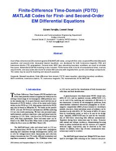
Problem: The investigated structure is shown in Fig. 1. It consists of a 200 nm wide, I 0 0 nm thick, variable length printed dipole. The dipole is placed at the interface between a dielectric substrate and the free space. A rectangular, non-uniform computational grid is used. A particular type of PML absorbing boundary condition, referred to as the uniaxial perfectly matched layer (UPML) introduced by Gedney [61, is used to truncate the computation domain. A delta gap scheme is used to excite the dipole with an I V amplitude, sine-modulated Gaussian Dipale pulse. The spectral content of the pulse covers the 8 to 12 micron domain. The simulation runs until the fields completely die down. An on-thefly discrete Fourier transform of both the driving voltage and the induced current is performed. The input impedance is given by the ratio of the voltage and current Fourier transforms. For every dipole length, the input impedance is Figure 1. Printed dipole antenna on a dielectric recorded substrate.
\
Approach: The FDTD algorithm is implemented on the workstation cluster by splitting the computation grid into equal subdomains. Each subdomain is assigned to a particular node in the cluster. The grid is split along the E planes. Each E plane contains two tangential electric field components and a perpendicular magnetic field component. To update the magnetic field component normal to the cutting plane, four tangential electric field components surrounding then H field are needed. Each subdomain has the necessary electric field components to do so. Therefore, there is no need for inter-node communication to update the magnetic field components. The magnetic field component normal to the cutting plane is redundantly updated by each of the neighboring nodes. Special consideration must be given to the two electric field components tangential to the cutting plane. Every node has only three of the four magnetic field components needed to update a tangential electric field component. Each node misses one Hx needed to update Ez and one Hz needed to update Ex. The missing magnetic field component needs to be retrieved from the neighboring node, leading to inter-node communication. For any cutting plane, two magnetic field components need to be interchanged, in our case Hz and Hx. Again, the two electric field components tangential to the cutting plane are redundantly updated by each of the two neighboring nodes. In the Beowulf cluster at IST, each node contains two processors. It runs LINUX and the MPICH implementation of Message Passing Interface standard is used for inter-node communication. To take advantage of the dual processors at each node, threaded programming is performed using the pthreads library. Within each node, the computation domain is further split along one plane. Each subdomain is assigned to one thread. Results: Figure 2a) shows the normalized run time versus the number of processors for a fixed size problem. Another way of viewing the same data is to use the so calledfixed speedup, computed as the ratio of the time it takes to run a problem on a processor to the time is takes to run the same problem on a given number of processors. Figure 2b) shows the fixed speedup versus the number of processors. As the number of processors increases, the fixed speedup curve deviates from a straight line and starts to saturate. Figure 2c) compares the fixed speedup for two different sized problems. As expected, the run time is Cut by almost a factor of two when going from one processor to two processors. However, there is not much to be gained by using eight or more processors for the smaller problem size shown, due to the increasing effect of communication latency. As the number of processors increases, each processor performs less computation but the same amount of communication. In other words, as the number of processors increases indefinitely for a fixed problem size, the communication time becomes large compared to the
1337
computation time. Note that the larger sized problem efficiently uses a larger number of processors, up to the limit of our system. To really take advantage of the parallelism of the FDTD, the problem size must be sufficiently large compared with the number of processors. Let us assume that the computation domain is going to be split along y = constant planes and the size of the problem that runs on a single processor is Nx*Ny*Nz. On a two processor run the problem size should be Nx*(2Ny)*Nz, on three processors Nx*(3Ny)*Nz and so on. In this situation, the scaled speedup is used to measure the performance of the parallel codes. The scaled speedup for P processors is defined as:
I
timetorunasizeS problemona processor timeto rua a size P * S problemon P processors An example of scaled speedup curve is shown in Fig. 2d). Note the highly linear character of the curve.
ssp(p) = p *
[
A given problem was run on the same number o f nodes, once using threads and once without threads. Figure 3a) shows the fixed speedup versus the number of nodes. When threads are used, each node contributes with two processors to the computation of the fields. The internode communication remains the same but the computation time is reduced by about of factor of two. Figure 3b) shows the fixed speedup vs. number of computing nodes for different threaded and non-threaded cases.
12 -
14
t121~50k50 10 -
-
.'
8-
I%i.
6:
8
4-
z6 I
0,
1338
4
24 20
--
1421~30k29 w h threads
-
4-
14.
w/ threads
P
16 -
111-
8
t ":
$
//) , I
p
/ I
// /"
8-
,I -
:/ '
8
'
I
,
L
1211j30k29 1421j30k291hr . .
0-
. a o
O
D
, o
B P
6-
2
l -
8 9
0
, . , . ,
,
2-
04 I
0
m
P /
( I "
I
.
12.
,
,
'
/
,
,
'
\
1339
0
o
2
d
,
6
. , a
,
IO
. 1,2
. , . , ii
16