Abstract. Current models of primary visual cortex (V1) include a linear filter- ing stage followed by a gain control mechanism that explains some of the nonlinear ...
Feature Coding with a Statistically Independent Cortical Representation Roberto Valerio1, Rafael Navarro1, Bart M. ter Haar Romeny2, and Luc Florack2 1
Instituto de Óptica “Daza de Valdés” - CSIC, Madrid, Spain, 28006 {r.valerio,r.navarro}@io.cfmac.csic.es 2 Faculteit Biomedische Technologie - Technische Universiteit Eindhoven Eindhoven, The Netherlands, 5600 MB {B.M.terHaarRomeny,L.M.J.Florack}@tue.nl
Abstract. Current models of primary visual cortex (V1) include a linear filtering stage followed by a gain control mechanism that explains some of the nonlinear behavior of neurons. The nonlinear stage has been modeled as a divisive normalization in which each input linear response is squared and then divided by a weighted sum of squared linear responses in a certain neighborhood. In this communication, we show that such a scheme permits an efficient coding of natural image features. In our case, the linear stage is implemented as a fourlevel Daubechies decomposition, and the nonlinear normalization parameters are determined from the statistics of natural images under the hypothesis that sensory systems are adapted to signals to which they are exposed. In particular, we fix the weights of the divisive normalization to the mutual information of the corresponding pair of linear coefficients. This nonlinear process extracts significant, statistically independent, visual events in the image.
1
Introduction
Traditional linear models of the responses of V1 neurons in primate visual cortex [1, 2] were highly attractive because of their simplicity, but they failed to explain essential nonlinear features of neural responses. In recent years, various authors have shown that the nonlinear behavior of V1 neurons can be modeled by including a gain control stage, known as divisive normalization [3, 4, 5, 6], after the linear filtering step. In this nonlinear stage the input linear responses are squared and then divided by a weighted sum of squared neighboring responses in space, orientation and scale, plus a regularizing constant. The hypothesis that sensory systems are adapted to the signals to which they are exposed implies that parameters of the divisive normalization are related to the statistics of natural images. More specifically, the efficient coding hypothesis [7] states that an efficient group of neurons should be able to encode as much information as possible, or in other words, that all their responses should be statistically independent. Different versions of this hypothesis were formulated by Barlow [8], who proposed that early sensory neurons remove statistical redundancy in the input signal, and by other authors [9, 10, 11, 12, 13]. Statistically-derived divisive normalization models have shown their utility to characterize the nonlinear response properties of typical neurons in sensory systems L.D. Griffin and M. Lillholm (Eds.): Scale-Space 2003, LNCS 2695, pp. 44–56, 2003. © Springer-Verlag Berlin Heidelberg 2003
Feature Coding with a Statistically Independent Cortical Representation
45
[14, 15, 16]. In addition, Simoncelli and Schwartz [14] showed that statisticallyderived divisive normalization reduces pairwise statistical dependences between output responses. It is well known that linear methods cannot eliminate higher-order statistical dependencies [e.g. 14, 17, 18]. Empirical results by Simoncelli and Schwartz [14] suggest that statistically-derived divisive normalization can significantly reduce higher order statistical dependencies between adjacent responses, which further supports the efficient coding hypothesis. In a recent paper, Hoyer and Hyvärinen [19] have used an alternative framework to show how the responses of V1 complex cells could be sparsely represented by a higher-order neural layer, which leads to contour coding and end-stopped receptive fields. In this communication, we use a statistically-derived divisive normalization model of the nonlinear information processing in V1 cells to obtain almost statisticallyindependent and sparse descriptors of natural images, which code relevant features in images. The main novelty of this scheme resides in the way of fixing the weights of the divisive normalization: each weight is fixed to the mutual information of the corresponding pair of linear coefficients. This is computationally more efficient.
2
Methods
2.1
Model of the Response of V1 Neurons
Following the current models of primary visual cortex (V1), the model proposed here consists of a linear decomposition followed by a nonlinear divisive normalization stage. 2.1.1 Linear Stage The linear stage is a four-level orthogonal wavelet decomposition based on Daubechies filters of order 4 (db8), that is with 4 vanishing moments and 8 coefficients [20]. The basis functions of this linear transform are localized in space, spatial frequency and orientation. This gives rise to 12 subbands (horizontal, vertical and diagonal for each of the 4 scales) plus an additional low-pass channel. Multi-scale and multiorientation orthogonal wavelet transforms like this are very popular for image representation. The marginal statistics of the resulting coefficients are known to be highly kurtotic and therefore non-Gaussian [e.g. 21, 22], and the joint statistics exhibit nonlinear dependencies. The left panel in Fig. 1 shows a typical orthogonal wavelet conditional histogram of a natural image. We can see that coefficients are decorrelated, since the expected value of the ordinate is approximately zero independently of the abscissa and therefore the covariance is close to zero as well. This makes an important difference between orthogonal and non-orthogonal linear transforms, since in the nonorthogonal cases “close” coefficients are correlated and the expected value of the ordinate is not zero but varies linearly with the abscissa. This is what we can see in the right panel in Fig. 1, which corresponds to a non-orthogonal Gabor pyramid [23].
46
Roberto Valerio et al.
Fig. 1. Conditional histograms of two neighbor coefficients (one is the vertical neighbor of the other) in the lowest (finest) scale vertical subband of the Daubechies (left), and Gabor (right) pyramid of the “Einstein” standard test image.
On the other hand, the “bowtie” shape of the left histogram reveals that coefficients are not statistically independent. This shape suggests that the variance of a coefficient depends on the value of the neighboring coefficient. The dependence is such that the variance of the ordinate scales with the squared value of the abscissa. All pairs of coefficients taken either in space, frequency or orientation always show this type of dependence [14, 17, 18], while the strength varies depending on the specific pair chosen. Intuitively, dependence will be stronger for coefficients that are closer, while it will decrease with distance along any axis. The form of the histograms is robust across a wide range of images, and different pairs of coefficients [15, 24]. In addition, this is a property of natural images but is not of the particular basis functions chosen [15]. Several distributions have been proposed in the context of V1 models to describe the conditional statistics of the coefficients obtained by projecting natural images onto an orthogonal linear basis [e.g. 15, 16]. Here we will consider a Gaussian model. Other closely related models have been proposed out of this context. Among them are the Gaussian Scale Mixture (GSM) models [e.g. 25, 26], which model a group of nearby wavelet coefficients as the product of two independent random variables: a scalar random variable and a zero-mean Gaussian random vector. Although GSM models permit, in theory, to get statistically independent coefficients through a nonlinear normalization, these models are not considered here because: first, this normalization procedure differs from the classical divisive normalization in V1 models and second, the Gaussian-distributed output coefficients that one would obtain, do not seem, intuitively, to be a proper model of the sparse responses of V1 neurons (for a discussion on sparse coding in V1 see [e.g. 27, 28]). Assuming a Gaussian model, the conditional probability p(ci | {c j }) of an orthogonal wavelet coefficient ci of a natural image, given the other wavelet coefficients {cj} (j ≠ i), can be modeled as a zero-mean Gaussian density with a variance that depends on a linear combination of the squared coefficients {c 2j } (j ≠ i) plus a constant ai2 , (ai2 +
∑b c j ≠i
ij
2 j
) [16]:
Feature Coding with a Statistically Independent Cortical Representation ci2 exp− 2 2 2 2 2 ( a b c ) + 2π (ai + ∑ bij c j ) ∑ i ij j j ≠i j ≠i
(1)
1
p (ci | {c j }) =
47
In the model, ai2 and {bij} (i ≠ j) are free parameters and can be determined by maximum-likelihood (ML) estimation. Operating with Eq. 1 we obtain the following ML equation: ci2 2 2 + log( ai + ∑ bij c j ) 2 2 j ≠i ai + ∑ bij c j j ≠i
{ai2 , bij } = arg min 2
{ai , bij }
where denotes expected value. In practice, we can compute averaging over all spatial positions of a set of natural images.
(2)
for each subband,
2.1.2 Nonlinear Stage The nonlinear stage consists basically of a divisive normalization, in which the responses of the previous linear filtering stage, ci, are squared and then divided by a weighted sum of squared neighboring responses in space, orientation and scale, {c 2j } , plus a constant, d i2 : ri =
(3)
ci2
d + ∑ eij c 2 i
2 j
j
Parameters d i2 and {eij} in Eq. 3 can be determined from the statistics of natural images if we accept the hypothesis that sensory systems are adapted to the statistical properties of the signals to which they are exposed [7, 8]. We will refer as optimal divisive normalization to the one defined by the values of the parameters (constant d i2 and weights {eij}) that yields the minimum mutual information, or equivalently minimizes statistical dependence, between normalized responses for a set of natural images. For a general formulation, we start from the definition of the mutual information, also called Kullback-Leibler divergence [29] of the normalized responses ri: +∞
MI (r1 , r2 ,..., rn ) = ∫ ... 0
∫
+∞ 0
p (r1 , r2 ,..., rn ) dr1 dr2 ... drn p (r1 , r2 ,..., rn ) log p (r1 ) ⋅ p (r2 ) ... p (rn )
(4)
If we use the change of variable theorem [30] to express the conditional probability density of the normalized responses p(r1, r2,…, rn) in terms of that of the linear inputs p(c1, c2,…, cn), and change the integration variables we get: MI ( r1 , r2 ,..., rn ) = +∞
= ∫ ... −∞
∫
+∞ −∞
c1 ⋅ c 2 ... c n ⋅ p (c1 , c 2 ,..., c n ) p (c1 , c 2 ,..., c n ) log r1 ⋅ r2 ... rn ⋅ p ( r1 ) ⋅ p ( r2 ) ... p ( rn ) ⋅ det [Id − E ⋅ R ]
(5) dc1 dc 2 ... dc n
48
Roberto Valerio et al.
where Id denotes the identity matrix, E the matrix of weights {eij}, and R the diagonal matrix of the normalized responses {ri}. And therefore the general expression for the set of parameters that minimizes the mutual information is: {d i2 , eij } = arg min MI (r1 , r2 ,..., rn ) = 2 { d i , eij }
= arg max 2
{d i , eij }
∫
+∞ −∞
...
∫
+∞ −∞
(6)
p (c1 , c2 ,..., cn ) log (r1 ⋅ r2 ... rn ⋅ p ( r1 ) ⋅ p (r2 ) ... p (rn ) ⋅ det[Id − E ⋅ R ] ) dc1dc2 ... dcn
In addition to the nice feature of giving statistical independent coefficients, the described model has another important property, namely it is invertible. Note that the linear stage is obviously invertible. Regarding the nonlinear stage (except for the signs, which need to be stored), we can reconstruct the squared input linear coefficients ci2 from the normalized responses ri and the parameters of the divisive normalization, d i2 and {eij}, by simply operating in Eq. 3. Since both stages, linear and nonlinear, of the nonlinear image representation scheme are invertible (if we keep the signs of the linear coefficients), it is possible to recover the input image from its nonlinear decomposition.
2
Results
In order to illustrate the features of the cortical code resulting from the above model we have undertaken some experiments with several standard test images. First, to model the conditional statistics of the orthogonal wavelet coefficients of an image, we used the Gaussian model in Eq. 1. We have studied the strength of the dependences between coefficients in space, frequency and orientation, finding that to a first approximation, most of the statistical dependence is concentrated within a neighborhood formed by adjacent coefficients. Thus, we considered in Eq. 1 the 299 coefficients {cj} (j ≠ i) adjacent to ci along the four dimensions (a 5x5 square box in the 2D space for each of the 12 subbands). An alternative way to determine which coefficients to include in the conditioning set, is to obtain the set of intraband and interband coefficients that minimizes the Kullback-Leibler divergence between the real conditional density of the wavelet coefficients and the statistical model of this density [24]. Once we have chosen the conditioning set, the Gaussian model non-negative parameters, ai2 and {bij} (i ≠ j), are adjusted in the following way, instead of using Eq. 2, for the sake of computational efficiency: ai2 is fixed to a small value (0.1) and {bij} (i ≠ j) are substituted by the mutual information of the corresponding pair of coefficients, ci and cj, calculated independently for each subband of the wavelet pyramid over all the coefficients of the input natural image. Note that this choice of parameters makes sense since ai2 is basically a regularizing constant to avoid dividing by zero, and the stronger the statistical dependence between two given coefficients, the greater is the corresponding bij parameter. As an example, Fig. 2 shows the resulting values of
Feature Coding with a Statistically Independent Cortical Representation
49
the {bij} (i ≠ j) parameters for the lowest (finest) scale vertical subband of the “Lena” image. In general, {bij} (i ≠ j) values are much less than one and highest values correspond to those neighboring coefficients in space, orientation and scale that have strongest statistical dependency with a certain coefficient.
Fig. 2. {bij} (i ≠ j) parameters for the lowest (finest) scale vertical subband of the “Lena” image. The 4 scales are vertically arranged (the lowest scale on top), and horizontally the 3 orientations (horizontal, vertical and diagonal on the left, in the middle and on the right respectively).
On the other hand, two considerations must be taken into account in order to efficiently attain an optimal divisive normalization that minimizes statistical dependence between output responses for natural images, that is, in order to efficiently solve Eq. 6. First, the mutual information of the normalized responses, MI(r1, r2,…, rn), (Eq. 4) does not depend on the value of the normalization parameters eii (it can be demonstrated that ∂MI (r1 , r2 ,..., rn ) = 0 , no matter the statistics of the linear inputs), so that ∂eii
these parameters can be fixed to any value (zero, say, for the sake of simplicity). Second, the choice of parameters d i2 = ai2 , eii = 0 and eij = bij, where ai2 and bij are the parameters of the Gaussian model (precisely the choice considered by Schwartz and Simoncelli in [16]) is an approximated solution of Eq. 6, easy to be computed, as it has been empirically demonstrated [16]. It is important to note that if we particularize the marginal probability of the normalized responses, p(ri), to that case, we obtain a highly kurtotic probability density function, which implies that the resulting code is sparse: p ( ri ) =
1 r ⋅ exp − i 2π ⋅ ri 2
(7)
When we apply the model described above, we obtain representations similar to that of Fig. 3.
50
Roberto Valerio et al.
Fig. 3. Lowest (finest) scale vertical subband of the Daubechies (middle row) and the nonlinear divisive normalization (bottom row) decomposition of the “Lena” image.
Intuitively, the nonlinear transform has the effect of randomizing the image representation in order to reduce statistical dependencies between coefficients belonging to the same structural feature, or in other words, the effect of the divisive normalization is to choose which coefficients are most effective for describing a given image structure, similarly to sparsification in those models based on an overcomplete and nonorthogonal basis set (see [27]). Fig. 4 represents three conditional histograms of two adjacent samples in space and illustrates the progressive statistical independence achieved by successive application of the linear (wavelet) and nonlinear (divisive normalization) transforms. The upper panel corresponds to the original image so that pi and pj are adjacent pixels (pj is the right down neighbor pixel of pi). The nearly 1 slope indicates the strong correlation between coefficients. The central panel shows the conditional histogram of the wavelet coefficients ci and cj. This linear transform cannot remove higher-order statistical dependencies, as suggested by the “bowtie” shape of the histogram. The bottom panel
Feature Coding with a Statistically Independent Cortical Representation
51
in Fig. 4 shows the conditional histogram between two adjacent output responses (ri and rj). After normalization, output statistical dependencies are practically removed since the resulting conditional histogram is basically independent on the value of the abscissa. Fig. 4 shows also a numerical evaluation of statistical dependence in terms of mutual information (Kullback-Leibler divergence). Consistently with Fig. 4, the mutual information, MI, is high, about 1.5, in the image domain. MI is much lower in the wavelet domain, after removing linear correlations. The divisive normalization further decreases MI to very low values close to zero. Table 1 illustrates the “robustness” of the model in the sense that results do not depend much neither on the parameters values, nor on the particular input natural image. Specifically, Table 1 shows some numerical measures of statistical dependence in terms of mutual information for 5 standard test images (“Boats”, “Elaine”, “Goldhill”, “Peppers” and “Sailboat”). As we can see, even if we use the parameters values previously calculated for the “Lena” image, the normalized responses are more statistically independent than the corresponding wavelet coefficients for any of the 5 images. Table 1. Mutual information between two neighboring wavelet coefficients ci and cj (cj is the right up neighboring coefficient of ci), and between the corresponding normalized responses ri and rj (using the parameters values of the “Lena” image), of 5 standard test images (see Fig. 5). The considered subband is always the lowest (finest) scale vertical one.
ci , cj
ri , rj
“Boats”
0.18
0.06
“Elaine”
0.05
0.04
“Goldhill”
0.10
0.03
“Peppers”
0.10
0.05
“Sailboat”
0.13
0.05
The effect of divisive normalization on marginal statistics is illustrated in Fig. 6. As we can see, the marginal density of the nonlinear responses, p(ri), is much more kurtotic, or in other words more peaked at zero, than the marginal density of the linear inputs, p(ci). In addition, we can observe that if we multiply the nonlinear responses by a certain constant k, the resulting marginal density p(ri’ = k·ri) closely fits the expression in Eq. 7, which is consistent with the assumption that MI(ci, cj) ≈ k•bij (i ≠ j) implicitly used in the model implementation.
52
Roberto Valerio et al.
MI = 1.55
MI = 0.13
MI = 0.03
Fig. 4. Conditional histograms and mutual information (MI) values of two neighboring pixels pi and pj (pj is the right up neighboring pixel of pi), wavelet coefficients ci and cj, and nonlinear responses ri and rj, of the “Lena” image. The considered subband is the lowest (finest) scale vertical one. Mutual information has been calculated from 200 bin joint histograms in the interval (-100 , 100) of the corresponding random variables after fixing their standard deviation (related to the mode) to 5 in order to compare the results.
Feature Coding with a Statistically Independent Cortical Representation
53
Fig. 5. Standard test images used in the experiments. From top to bottom and left to right: “Boats”, “Einstein”, “Elaine”, “Goldhill”, “Lena”, “Peppers” and “Sailboat”.
54
Roberto Valerio et al.
Fig. 6. Left panel: Marginal density functions of wavelet coefficients (ci) and of nonlinear responses (ri) in the lowest (finest) scale vertical subband of the “Lena” image. Right panel: Density function of the nonlinear responses in the lowest (finest) scale vertical subband after multiplying them by a certain constant k. With x’s it is represented . p ( ri ) =
3
1 2π ⋅ ri
r ⋅ exp − i 2
Conclusions
We have used a statistically-derived model of the nonlinear information processing in V1 neurons to illustrate some features of the cortical code. The key principle is the efficient coding hypothesis, that is, that the resulting responses should be as statistically independent as possible. One of the main contributions is the method for obtaining the parameters values of the model nonlinear step. Basically, d i2 is fixed to a small value (0.1) and {eij} (i ≠ j) are substituted by the mutual information of the corresponding pair of coefficients, ci and cj. This method is computationally efficient and thus permits to consider a large set of neighboring coefficients. Numerical results constitute the empirical proof for both the theoretical formulation and the validity of the numerical procedures, and suggest that the statisticallyindependent and sparse cortical code is a very efficient representation of the most frequent features of natural images. The model is robust in the sense that results do not depend much on the linear orthogonal decomposition, the model of the conditional statistics of the linear coefficients, the training set of natural images, the computing errors (for example in estimating the parameters), or even the particular input natural image. Finally, this nonlinear scheme of image representation, which has better statistical properties than the popular orthogonal wavelet transforms, is potentially useful for many image analysis and processing applications, such as restoration, synthesis, fusion, coding and compression, registration, etc., because of its invertibility and the great importance of statistical independence in these applications. Similar schemes [18, 31] have already been used very successfully in image analysis and processing applications.
Feature Coding with a Statistically Independent Cortical Representation
55
Acknowledgments This research was supported by the Spanish Commission for Research and Technology (CICYT) under grant DPI2002-04370-C02-02. Roberto Valerio was supported by a Madrid Education Council and Social European Fund Scholarship for Training of Research Personnel, and by a City Hall of Madrid Scholarship for Researchers and Artists in the Residencia de Estudiantes.
References 1. D. Hubel, and T. Wiesel, “Receptive fields, binocular interaction, and functional architecture in the cat’s visual cortex”, J. Physiol (Lond), 160, pp. 106-154, 1962. 2. J. A. Movshon, I. D. Thompson, and D. J. Tholhurst, “Spatial summation in the receptive fields of simple cells in the cat’s striate cortex”, J. Physiol (Lond), 283, pp. 53-77, 1978. 3. A. B. Bonds, “Role of inhibition in the specification of orientation selectivity of cells in the cat striate cortex”, Visual Neuroscience, 2, pp. 41-55, 1989. 4. W. S. Geisler, and D. G. Albrecht, “Cortical neurons: Isolation of contrast gain control”, Vision Research, 8, pp. 1409-1410, 1992. 5. D. J. Heeger, “Normalization of cell responses in cat striate cortex”, Visual Neuroscience, 9, pp. 181-198, 1992. 6. M. Carandini, D. J. Heeger, and J. A. Movshon, “Linearity and normalization in simple cells of the macaque primary visual cortex”, J. Neuroscience, 17, pp. 8621-8644, 1997. 7. F. Attneave, “Some informational aspects of visual perception”, Psych. Rev, 61, pp. 183193, 1954. 8. H. B. Barlow, “Possible principles underlying the transformation of sensory messages”, Sensory Communication, p. 217, MIT Press, 1961. 9. S. B. Laughlin, “A simple coding procedure enhances a neuron’s information capacity”, Z. Naturforsch, 36C, pp. 910-912, 1981. 10. J. J. Atick, “Could information theory provide an ecological theory of sensory processing?”, Netw. Comput. Neural Syst., 3, pp. 213-251, 1992. 11. J. H. van Hateren, “A theory of maximizing sensory information”, Biol. Cybern., 68, pp. 23-29, 1992. 12. D. J. Field, “What is the goal of sensory coding?”, Neural Comput., 6, pp. 559-601, 1994. 13. F. Rieke, D. A. Bodnar, and W. Bialek, “Naturalistic stimuli increase the rate and efficiency of information transmission by primary auditory afferents”, Proc. R. Soc. London B, 262, pp. 259-265, 1995. 14. E. P. Simoncelli, and O. Schwartz, “Modeling Surround Suppression in V1 Neurons with a Statistically-Derived Normalization Model”, Advances in Neural Information Processing Systems, 11, pp. 153-159, 1999. 15. M. J. Wainwright, O. Schwartz, and E. P. Simoncelli, “Natural image statistics and divisive normalization: modeling nonlinearities and adaptation in cortical neurons”, Statistical Theories of the Brain, eds. R. Rao, B. Olshausen, and M. Lewicki, MIT Press, 2001. 16. O. Schwartz, and E. P. Simoncelli “Natural signal statistics and sensory gain control”, Nature neuroscience, 4(8), pp. 819-825, 2001. 17. B. Wegmann, and C. Zetzsche, “Statistical dependence between orientation filter outputs used in an human vision based image code”. Proc. SPIE Vis. Commun. Image Processing, pp. 1360, 909-922, Soc. Photo-Opt. Instrum. Eng, Lausanne, Switzerland, 1990.
56
Roberto Valerio et al.
18. E. P. Simoncelli, “Statistical Models for Images: Compression, Restoration and Synthesis”, Asilomar Conf. Signals, Systems, Comput., pp. 673-679, IEEE Comput. Soc, Los Alamitos, CA, 1997. 19. P. O. Hoyer, and A. Hyvärinen, “A multi-layer sparse coding network learns contour coding from natural images”, Vision Research, 42(12), pp. 1593-1605, 2002. 20. I. Daubechies, Ten Lectures on Wavelets, CBMS-NSF Lecture Notes nr. 61, SIAM, 1992. 21. D. J. Field, “Relations between the statistics of natural images and the response properties of cortical cells”, J. Opt. Soc. Am. A, 4(12), pp. 2379-2394, 1987. 22. S. G. Mallat, “A theory for multiresolution signal decomposition: The wavelet representation”, IEEE Pat. Anal. Mach. Intell., 11, pp. 674-693, 1989. 23. O. Nestares, R. Navarro, J. Portilla, and A. Tabernero, “Efficient Spatial-Domain Implementation of a Multiscale Image Representation Based on Gabor Functions”, Journal of Electronic Imaging, 7(1), pp. 166-173, 1998. 24. R. W. Buccigrossi, and E. P. Simoncelli, “Image compression via joint statistical characterization in the wavelet domain” IEEE Transactions on Image Processing, 8(12), pp. 1688-1701, 1999. 25. M. J. Wainwright, and E. P. Simoncelli, “Scale Mixtures of Gaussians and the Statistics of Natural Images”, Advances in Neural Information Processing Systems, 12, pp. 855-861, 2000. 26. M. J. Wainwright, E. P. Simoncelli, and A. S. Willsky, “Random Cascades on Wavelet Trees and Their Use in Modeling and Analyzing Natural Imagery”, Applied and Computational Harmonic Analysis, 11(1), pp. 89-123. 27. B. A. Olshausen, and D. J. Field, “Sparse coding with an overcomplete basis set: A strategy employed by V1?”, Vision Research, 37, pp. 3311-3325, 1997. 28. B. A. Olshausen, “Sparse Codes and Spikes”, Statistical Theories of the Brain, eds. R. Rao, B. Olshausen, and M. Lewicki, pp. 257-272, MIT Press, 2002. 29. S. Kullback, and R. A. Leibler, “On information and sufficiency”, The Annals of Mathematical Statistics, 22, pp. 79-86, 1951. rd 30. A. Papoulis, Probability, random variables and stochastic processes (3 ed.), McGrawHill, Inc, Singapore, 1991. 31. J.Malo, F. Ferri, R. Navarro, and R. Valerio, “Perceptually and Statistically Decorrelated Features for Image Representation: Application to Transform Coding”. Proceedings of the 15TH International Conference on Pattern Recognition, 3, pp. 242-245, IEEE Computer Society, Barcelona, Spain, 2000.