Turkish Journal of Electrical Engineering & Computer Sciences http://journals.tubitak.gov.tr/elektrik/
Research Article
Turk J Elec Eng & Comp Sci (2018) 26: 2886 – 2899 © TÜBİTAK doi:10.3906/elk-1611-297
Feature extraction using sequential cumulative bin and overlap mean intensity for iris classification Ahmad Nazri ALI∗,, Shahrel Azmin SUANDI,, Mohd Zaid ABDULLAH, School of Electrical and Electronic Engineering, Universiti Sains Malaysia, Engineering Campus, Penang, Malaysia Received: 29.11.2016
•
Accepted/Published Online: 30.06.2018
•
Final Version: 29.11.2018
Abstract: This paper examines an approach generalizing a variant of the local binary pattern (LBP) method for iris feature extraction. The proposed method employs two different LBP variants called the sequential cumulative bin and overlap mean intensity for projecting the one-dimensional local iris textures into a binary bit pattern. The assigned bit, either 1 or 0 as a bit code, replaces the original intensity value using a specific condition for the respective reference element. The ratio value from the total transition of 1 to 0 along the row axis represents the feature of each iris image. The extraction only utilizes a small area of interest on the iris image that covers parts of the iris textures with minimum eyelid and eyelashes. The assessment employs the support vector machines classifier and the result demonstrates a good classification rate with average accuracy of 94.0% for the individual mode. However, the classification rate has improved to reach 96.5% accuracy if the assessment uses a concatenated mode set of features. Besides that, increasing the amount of samples in the training data by using the synthetic together with the original samples has also been able to improve the classification rate. Key words: 1D-Local binary pattern, histogram equalization, support vector machines, iris classification
1. Introduction Iris recognition or classification is a method to differentiate between individuals using tiny textures and unique patterns in the iris. Each person has dissimilar patterns even between the left and right eye. A well-known iris classification system is the one suggested by Daugman [1,2]. Since then, many researchers have worked in this field, resulting in improved techniques, and their performances are comparable to Daugman’s work. Reliable features are the key element for obtaining high accuracy. In order to obtain reliable features, the unwanted noises caused by the eyelid and eyelash must be masked and eliminated so that these attributes will not be figured as genuine iris information during feature extraction. There are several eyelid and eyelash removal methods that have been proposed, and most of the methods are performed before the extraction process [3–5]. A unique representation of each individual must be produced from the iris textures in order to classify or identify the person. The iris code proposed by Daugman contained bits 1 and 0 and was the earliest representation for iris textures. Over the years and in current practice [6–16], most of the methods generate the features from a two-dimensional domain of the iris image and then project it into real values or a binary representation. Finding local attributes for iris descriptors is common practice at the feature extraction level in iris recognition [17–19]. Local binary pattern (LBP) is the prevalent approach that uses local information of images for features, and it has been widely used in various application areas including face, texture, and iris ∗ Correspondence:
[email protected]
2886 This work is licensed under a Creative Commons Attribution 4.0 International License.
ALI et al./Turk J Elec Eng & Comp Sci
recognition as well [20–23]. First introduced by Ojala et al. in 1996, this basic LBP operator was generalized to multiscale and multisampling variants of LBP [24]. It is denoted as LBP P,R , where R and P are the radius and the number of neighborhoods, respectively. In general, the equation to calculate the LBP operator is defined by Eqs. (1) and (2) [24]. LBP P,R =
[P −1 ∑
] s (gi −gc ) 2i
(1)
i=0
{ where, s (x) =
1 0
if x≥ 0 Otherwise
(2)
gi is the intensity value at the i th neighborhood from the central element, gc . The neighborhood pixels are converted to 0 if the pixel gray level is smaller than the center pixel. Otherwise, they are converted to 1. Multiplying the converted values by 2n (n is the index from 0 to 7 for the case of the eighth neighborhood), which is read sequentially in a clockwise direction, and summing up the result will produce the LBP operator for the center pixel. Classifying the texture or information by adapting the 2D classical LBP to 1D signal has also been introduced in several works. For example, 1D-LBP has been used to extract the features in speech recognition systems [25,26], EEG signals [27,28], and bone texture characterization [29]. For one-dimensional LBP, the operator is defined by comparing the center value with its neighboring values along one axis only. Normally N /2 neighboring values are considered for the left or right position from the center value. A similar rule as in two-dimensional is used to assign the binary number to each neighboring pixel, regarding the weighted values to each index for the operator computation. To obtain a satisfactory classification result, a robust feature extraction method is required, particularly if the feature is extracted at a specific region because it may contain insufficient information for the required features. Therefore, in this paper, an effective approach using the state-of-the-art LBP is proposed for iris feature extraction. The method will extract the iris information from a selected region that comprehends with less or no unwanted noises due to eyelid or eyelashes. The ratio of the specific bitwise transition along the horizontal axis will be computed for the feature descriptors. The paper is subdivided into the following sections: Section 2 presents an overview of the suggested 1D-LBP approach. Following this, Section 3 delivers the experimental results and the discussion, and finally Section 4 presents the conclusion. 2. The proposed 1D-local binary pattern for feature extraction In this paper, we propose a new extended variant of 1D-LBP that adapts the model of the classical 1D-LBP to classify iris images. The proposed 1D-LBP requires two computation levels before finalizing the bit decision to the reference element. The 1D-LBP code is defined by selecting the majority bit in the bitwise stream from the neighborhood set. The key idea for the proposed 1D-LBP is to convert each pixel (element) in the selected region with binary bit number either 1 or 0. In classical 1D-LBP, the binary code for all possible linearly symmetric neighborhood sets is calculated by thresholding the value to the central element. However, in the proposed method, the central element is replaced with the leftmost value in the neighborhood set for a reference element. 2887
ALI et al./Turk J Elec Eng & Comp Sci
Since the proposed LBP uses the pixels along the horizontal side with a particular number of neighborhoods, the smooth transition computation for the angular iris attributes can be performed in order to obtain precise inference between neighborhoods. One of the main impacts of using the proposed LBP is in terms of the iris region selection, where only a small partial iris region is required for generating reliable iris features. The selected regions generally contain none or a minimum amount of the unwanted attributes, and the algorithms can process the iris attributes without any noise removal method in order to produce the features. This is dissimilar to most of the previous works, in which noise removal groundwork is required before further feature extraction. Having both elements (small iris region and noise removal algorithm), it will be able to reduce the execution overhead in order to complete an entire iris classification system. In order to realize the approach, a small iris region is set for the binary bit projection (Figure 1). A histogram equalization (HE) method is applied to the selected area, and by having the probability density function, p [x] and cumulative distribution function, Cx , the texture enhancement is performed using Eq. (3) [30].
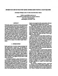
Figure 1. Examples of the image with constant location and dimension.
The = (Cx (i) − (0.5 × p [x])) × imax
(3)
Here, imax is the maximum elements’ intensity detected in the input image. The is the value that will compute the previous corresponding element value, i. The main purpose of the HE is to enhance the contrast of the background noise and at the same time to improve the iris textures’ appearance, as shown in Figure 2. With the textures’ improvement, it provides a sufficient possibility for the proposed LBP to extract the important features and this makes the HE become a very important stage in this study in order to achieve high performance classification rates.
Figure 2. Examples of the image before (left) and after (right) HE.
2.1. Sequential cumulative bin In the first variant, called the sequential cumulative bin (SCB), we formed a linear attribute of size Z that sequentially reads the values with one element step to the right, thresholding these values to the reference (the leftmost element) in order to assign a bit number to each respective neighborhood element. Figures 3a– 3c illustrate the three possible linearly sequential neighbor sets for the different values of Z while Figure 4 diagrammatically illustrates the first level of the SCB method, where the neighborhood values are projected onto the bit number relative to the leftmost (reference) value. In Figure 4, since bit 1 is the majority bit in the stream, this bit will be assigned to the reference element as a replacement for the previous value. However, if an equal majority bit occurs (for the case of 4 and 6 neighborhood elements), the decision is made by considering the average value for all the respective 2888
ALI et al./Turk J Elec Eng & Comp Sci
PTR
P0
P1
P2
P3
PTR
P0
P1
(a)
P2
P3
P4
PTR
(b)
P0
P1
P2
P3
P4
P5
(c)
Figure 3. Linearly sequential neighbor sets with (a) Z = 4, (b) Z = 5, (c) Z = 6.
neighborhoods and then rethresholding with the reference for the bit projection. The SCB 1D-LBP bit projection can be defined by Eqs. (4) and (5). P TR 24
P0 45 1
P1 35 1
P2 47 1
P3 45 1
P4 21 0
P5 47 1
P6 50 1
Binary (1111011) Bit 1 is the majority in the bit stream 1
Figure 4. SCB 1D-LBP code projection process.
Z−1 1DLBP SCB Z = majority (1, 0) |i=0 v(Pi − PT R )
{ where, v (x) =
1 if x ≥ 0 0 if x < 0
(4)
(5)
In Eq. 4, Pi is the i th neighborhood element, Z is the number of neighbor sets used for projection, and PT R is the reference element. The representation of 1D iris patterns is modeled by a ratio for the bitwise transition from 1 to 0 along the horizontal axis and it is computed for individual feature descriptors. With this approach, a set of feature vectors will be produced where the number of the vectors generally follows the size of the vertical axis of the selected region ( y -axis). The calculation for the individual descriptor can be defined using Eqs. (6) and (7). U=
j ∑
X [1]i →X[0]i+1
(6)
i=0
F m =Um /m
(7)
Here, j and m are the horizontal and vertical dimension values while X [ 1 ] and X [ 0 ] are the i th elements with bit 1 and 0, respectively. Um is the amount of bit transition counted along the horizontal at particular vertical mwhile Fm is the bit transition ratio at vertical m , which represents a features vector. 2.2. Overlap mean intensity The second variant is called the overlap mean intensity (OMI). It involves the average distribution and requires two phases of computation before the bit is projected to the reference element. This variant applies a similar concept as in 1D-LBP SCB for bit projection and feature representation. In the first phase, the preinitial average values will be calculated for each block of the consecutive neighboring elements. However, for the second and remaining blocks, the last element in each block will be reused with the next block for another preinitial average 2889
ALI et al./Turk J Elec Eng & Comp Sci
computation. An example of the progression of this variant is illustrated in Figure 5 with two elements for each block and three significant preinitial average values. PTR
P0
P1
P2
P3
24
45
35
47
45
X1
24
X2
40
X3
41
24
46
42 24 – 42 < 0 then P TR → 0
PTR
P0
P1
P2
P3
0
Figure 5. 1D-LBP OMI code projection process.
Average computation is used to fold any smooth or irregular texture intensity in the neighborhood region and then uses bit assignment to indicate the intensity variance for the reference. If the reference element is greater or less than the average value, it means that sufficient intensity difference exists between the elements, even in the case of a small difference between the reference elements and the average intensity. To obtain adequate smooth texture and minimize the incorrect element intensity difference, the denominator, N , in Eq. (8) must be similar to the amount of elements used for the average computation. To find the intensity difference between the reference and the neighborhood overall mean, Eq. (9) is used, with M the number of the calculated average (for example, in Figure 4, M is 3). In general, the OMI variant can be represented by Eqs. (8)–(10). Xi =
1 N
i=i+(N −1)
∑
Pi−1
(8)
i=i
1 ∑ Xi M + 1 i=0 M
Tj = PT R −
{ where, Tj =
1 if Tj ≥ 0 0 if Tj < 0
(9)
(10)
In Eq. (8), X i is the ith preinitial average value. Meanwhile, T j in Eq. (9) is the j th corresponding reference element for bit projection. Generally, both variants are used to find a local correlation between the neighboring elements, whereby the feature descriptor provides eloquent pattern transition information (from the amount of bit transition) for the specified iris textures along the horizontal axis. 2890
ALI et al./Turk J Elec Eng & Comp Sci
3. Experimental results and discussion In this study, we employ an SVM classifier to evaluate the proposed SCB and OMI 1D-LBP variants. Generally, SVM is a machine learning approach widely used for classification or recognition. In the iris recognition field, SVMs have been employed using various kinds of feature schemes with proven performance [31,32]. The key behind SVMs is the kernel function that maps the data from the input space to the higher dimensional feature space, which is designed to make the data points linearly separable. Four types of kernels consisting of linear, polynomial, RBF, and sigmoid are used for assessing the proposed method. In order to achieve high performance accuracy, suitable training data, optimum penalty, and kernel parameters have been chosen during the training session. The method called leave-one-out cross-validation is applied for training data selection in order to obtain a satisfactory classifier (SVM model) for a high performance rate. Three freely available databases, which are CASIA (Chinese Academy of Sciences Institute of Automation) V1 (108 subjects), CASIA V3 (249 subjects), and IITD (Indian Institute of Technology Delhi) (224 subjects), were used to evaluate the performance of the proposed methods. For assessment, we have selected three best samples from each subject for training and the remainder was for testing. Stand-alone and concatenate mode iris features were considered in our assessment. Two multiclass classification approaches based on one-versus-one (OVO) and one-versus-all (OVA) were used to assess the proposed method. The OVO approach is a method to construct the x (x − 1) /2 binary classifier of two classes trained with two by two subjects. For the OVO classification, the SVM model is trained using a dataset consisting of six samples from two different subjects. Each subject is assigned as either positive or negative class. A voting scheme is applied for the testing samples and the class that gives the highest number with positive predictions will be selected as the correct classified subject. Meanwhile, in the OVA approach, which is a method to build x SVM classifier models, the ith classifier is trained with the ith class coded as positive and the rest of the training samples are coded as negative. In the OVA approach, each training dataset is formed based on the combination of three positive samples from one subject and some amount of negative samples from a few different subjects. Based on this combination, it will produce a trained model that may be biased towards the majority (negative) during classification, because the model is trained with imbalanced samples between positive and negative classes. With the OVA approach, we believe that the outcome may provide a decent indication of the proposed method, particularly the features’ reliability in an imbalanced learning environment. Since HE is one of the important stages for better performance, as mentioned in Section 2, a preliminary experiment using the OVO classification scheme on the SCB method with only 25 subjects of each related database has been performed in order to prove its significance. Only the linear kernel is preferred for the assessment and the features are extracted from an image size of 140 ×30 for 6 neighborhoods. The result of this evaluation is shown in Table 1. It can be seen clearly that the proposed LBP method requires the HE scheme at an early stage in order to achieve an acceptable classification rate.
Table 1. Classification rate with and without HE on SCB method (linear kernel).
Database CASIA v1 CASIA v3 IITD
Classification Without HE 4.16 8.33 7.30
rate, % With HE 93.75 91.66 90.62 2891
ALI et al./Turk J Elec Eng & Comp Sci
Having the outcome after HE scheme evaluation, we then continue the assessment to the remaining iris images and it is found that results of satisfactory outcomes are achieved for all types of kernels in the OVO classification approach. This is presented in Table 2, where the concatenated mode shows an improvement in outcome compared to the stand-alone mode for all the database and kernels. For the stand-alone mode, it was found that the result for the OMI method is better with a small increment compared to the SCB variant. Meanwhile, for the OVA classification approach, a satisfactory outcome was also achieved, and the result of this type of classification is shown in Table 3. Again, the result for the concatenated mode is higher than for the stand-alone, but the overall rate is slightly lower compared to the OVO approach for both assessment modes. We have also conducted an additional assessment with several different neighboring elements for both the SCB and OMI in order to observe the performance with respect to the number of neighboring elements, and also for different individual ( X) and adjacent mean ( P ) just for the OMI variant. By limiting the number of neighboring elements ( P ) to seven, it produced a maximum of five and four individual means in the case of three and four elements, respectively. From our observation, based on these two separate mean calculations, we found that in order to obtain a better classification performance, at least three adjacent means were needed for the descriptor computation. The results of these experiments are tabulated in Table 4 and Table 5, respectively. We only choose the OVO classification as a preliminary evaluation for this case as we assume that all the changes made in terms of the number of neighboring elements, various individuals, and adjacent mean will not provide a high impact on the performance of the OVA classification and the concatenate mode. We predicted that a similar performance pattern could be achieved if we take note of the previous results. In Table 4, it can be seen that the neighboring 7 elements are the best amount that would be appropriate to be used for the average computation in both the proposed methods. If the number of neighboring elements is less than five, it may contribute to a diminutive correlation between the neighboring elements and not much information of interest will be obtained from the bit stream. A similar case can also be seen for more than seven, where the reference is correlated with the elements that are far from it, which may contain incoherent attributes between them. For the number of individual and adjacent mean computations (in the OMI case), it is found that only two values (3 and 4) have achieved a satisfactory outcome, as presented in Table 5. If the value for the individual mean computation is increased, it will require more neighboring elements, which may yield a poor average with a deficiency in meaning in order to associate the iris texture relationship. A similar case can be seen in the adjacent mean as we can see that the performance decreases when the adjacent is increased to 5 and a worse performance arises (indicated by X) if the individual mean is set to 4 due to the increment of the neighboring elements used for computation. Meanwhile, Figures 6a–6d show the results for different combinations of the vertical (y-axis) and the horizontal size (x-axis), where it can be concluded that the ranges from 20 to 34 for the vertical and 120 to 160 for the horizontal are the most considerable image sizes for an excellent performance. Generally, an average classification score measurement can be illustrated by an ROC curve, as shown in Figure 7, in which the area under the curve (AUC) indicates that both methods can be good techniques to classify iris texture. However, the proposed methods have insignificant shortcomings since it cannot be tolerated for robust feature formation if the selected region contains more noises attributes. From the two variants, it is found that the performance for the OMI variant is better than the SCB in a single assessment. Based on the nature of the computation, the SCB method may produce features with less pattern separation but enough to cultivate the contrast difference between the neighboring elements. One drawback of the SCB method is that if the selected elements contain high contrast intensity between them, such as from the 2892
CASIA V1 CASIA V3 IITD
Database
CASIA V1 CASIA V3 IITD
Database rate (%) Linear 93.6 92.7 94.8 RBF 92.7 91.5 93.6
Sigmoid 92.7 91.5 93.6
OMI Classification Polynomial 94.6 92.7 94.8 rate (%) Linear 94.6 92.7 94.6 RBF 92.7 92.7 93.4
Sigmoid 92.7 92.7 92.9
Concatenate variant Classification rate (%) Polynomial Linear 96.2 96.5 95.5 95.7 96.2 96.2
Method SCB Classification Polynomial 92.9 90.2 94.8 rate (%) Linear 92.9 90.2 94.6 RBF 90.2 90.4 92.9
Sigmoid 90.4 90.4 92.9
OMI Classification Polynomial 92.7 91.5 94.0 rate (%) Linear 92.7 91.3 94.6
RBF 89.7 89.7 90.2
Sigmoid 89.4 89.4 92.7
Concatenate variant Classification rate (%) Polynomial Linear 95.7 95.5 93.9 93.6 96.2 96.2
Table 3. Result of classification for one versus all approach for the image size of 140 ×30.
Method SCB Classification Polynomial 93.9 92.7 94.6
Table 2. Result of classification for one versus one approach for the image size of 140 ×30.
RBF 93.6 93.4 94.8
RBF 94.8 95.7 96.0
Sigmoid 93.6 93.6 94.6
Sigmoid 94.6 95.5 96.0
ALI et al./Turk J Elec Eng & Comp Sci
2893
ALI et al./Turk J Elec Eng & Comp Sci
Table 4. Average classification rate for several neighboring pixels on different sizes of the selected iris region.
Average classification rate, % Database
Variants
Kernel Polynomial Linear RBF Sigmoid Polynomial Linear RBF Sigmoid Polynomial Linear RBF Sigmoid Polynomial Linear RBF Sigmoid Polynomial Linear RBF Sigmoid Polynomial Linear RBF Sigmoid
SCB CASIA V1 OMI
SCB CASIA V3 OMI
SCB IITD OMI
Number of 2 3 1.0 11.0 1.0 10.5 1.0 10.0 1.0 10.0 1.5 32.5 1.5 32.5 1.5 30.0 1.5 30.0 0.5 10.0 0.5 10.0 0.5 9.0 0.5 9.0 1.5 30.0 1.5 30.5 1.0 29.5 1.0 29.5 1.0 16.5 1.0 18.0 1.0 17.0 1.0 17.5 2.5 35.5 2.5 36.0 2.0 36.0 2.0 36.0
neighboring pixels 4 5 6 62.5 92.5 93.5 62.5 93.0 93.5 62.0 91.0 92.5 62.0 91.0 92.5 64.5 93.5 94.0 64.5 93.0 94.0 64.0 92.0 93.0 64.0 92.0 93.0 61.5 91.5 92.5 61.5 92.5 92.5 60.0 91.0 92.0 60.0 91.0 92.0 61.5 92.0 92.0 61.5 92.0 92.5 61.0 91.0 90.0 61.0 91.0 90.0 63.5 93.5 94.5 63.5 94.0 94.0 63.0 92.0 93.0 63.0 92.0 93.0 64.0 94.0 94.0 64.0 94.0 94.0 64.0 92.0 94.0 64.0 92.0 94.0
7 93.5 93.5 92.5 92.5 94.5 94.5 92.5 92.5 92.5 92.5 91.5 91.5 92.5 92.5 92.5 92.5 94.0 94.0 93.0 93.0 94.0 94.0 93.0 92.0
8 88.5 88.5 85.0 85.0 89.5 89.5 88.0 88.0 86.5 86.5 85.0 85.0 90.0 90.0 89.0 89.0 90.5 90.5 89.0 89.0 90.0 90.0 90.0 90.0
Table 5. Average classification rate, %, for various individual means and adjacent means.
Individual mean 3 4
Adjacent mean 3 4 5 94.5 94.0 93.5 94.5 94.0 X
eyelashes and the iris texture, then it may produce inaccurate bit determination for the reference. However, for the OMI, since it uses a two-level average scheme, if the above-mentioned situation occurs, the computation can blend the eyelashes’ intensity. As a result, the consequence for the wrong final bit projection is less because all the eyelash intensities will be balanced by neighboring elements. If the selected region contains more eyelid or eyelash information than the iris texture, then it may generate a redundant bit, but the chances of this situation happening are low 2894
ALI et al./Turk J Elec Eng & Comp Sci
100 (a)
95
Vertical Size - 20
90 85 80 75
CASIA V1 (SCB) CASIA V3 (SCB) IITD (SCB) CASIA V1 (OMI) CASIA V3 (OMI) IITD (OMI)
70 65
Vertical Size - 26
(b)
Classification Accuracy, %
Classification Accuracy, %
100
60
95 90 85 80 CASIA V1 (SCB) CASIA V3 (SCB) IITD (SCB) CASIA V1 (OMI) CASIA V3 (OMI) IITD (OMI)
75 70 65
60
80
100 120 140 160 180 200 220 240 260
60
80
100 120 140 160 180 200 220 240 260
Horizontal Size
Horizontal Size 96 Vertical Size - 30
(c)
94
Classification Accuracy, %
Classification Accuracy, %
96
92 90 88 86
CASIA V1 (SCB) CASIA V3 (SCB) IITD (SCB) CASIA V1 (OMI) CASIA V3 (OMI) IITD (OMI)
84 82
Vertical Size - 34
(d)
94 92 90 88 86
CASIA V1 (SCB) CASIA V3 (SCB) IITD (SCB) CASIA V1 (OMI) CASIA V3 (OMI) IITD (OMI)
84 82 80
80 60
80
100 120 140 160 180 200 220 240 260
60
80
100 120 140 160 180 200 220 240 260 Horizontal Size
Horizontal Size
Figure 6. Classification accuracy with different horizontal dimensions for vertical size of (a) 20, (b) 26, (c) 30, (d) 34.
True Positive Rate (Sensitivity)
1.0
0.8
0.6 CASIA V1 CASIA V3 IITD
0.4
0.2
0.0 0.0
0.2
0.4
0.6
0.8
1.0
False Positive Rate (1-Specificity)
Figure 7. ROC curve for the concatenated mode for the image size of 140 ×30.
as the selected size for the extraction contains none or less of the unwanted noise. Feature concatenation from both methods exhibits strong efforts to cover any mistaken bit projection. The concatenate mode has caused the feature vector to increase, but it is able to recuperate any unseen features that cannot be extracted by one of the methods. 2895
ALI et al./Turk J Elec Eng & Comp Sci
Besides the above assessments, we have also conducted a preliminary study to observe the consequence of number of samples in the training data for the classification rate. Due to the samples in each database being limited, we used the image deformation technique to augment the samples. Acceptable warping with random displacement to the image pixel (based on the grid) is applied for producing synthetic samples. For initial assessment, 70 synthetic samples are created for each subject from 25 selected subjects of each database. Several training datasets are formed based on the combination of some amount of synthetic (15 and 35 samples) and original samples (0, 1, and 2 samples). A similar experimental setup for model generation as conducted in HE assessment has been considered for the study. In this experiment, the classification score is recorded when testing is performed for the generated model by using the testing samples as applied in the previous experiments. The results for this experiment are tabulated in Table 6. Table 6. Classification rate, %, of the original samples when tested with the model created using some amount of the original and synthetic samples.
Database
CASIA V1 CASIA V3 IITD
Number of synthetic and the training data 15 0 1 2 90.31 97.63 100 88.81 96.86 100 91.36 97.76 100
original samples in the 35 0 91.02 89.21 92.13
1 98.26 97.93 98.56
2 100 100 100
From the table, it is found that to achieve a good classification rate, at least one original together with 15 synthetic samples are required in the training data. Without original samples in the training data, the result is unsatisfactory, although we have increased the amount of the synthetic samples. It can also be seen that with at least one original sample, the classification rate has improved if the amount of the synthetic samples is increased from 15 to 35 samples. It was found that if a minimum of 2 original samples are added in the training data, then the score is able to reach up to 100% accuracy. It was also found that both synthetic and original samples are jointly required in the training data for achieving a satisfactory performance. Based on the results obtained from all the performed experiments, it is observed that the performance of the proposed method is comparable with the existing works if the finding is associated according to the variants of the LBP approach as tabulated in Table 7. The outcome of the proposed method is also promising if the comparison is made based on different frameworks of extraction methods as depicted in Table 8. In fact, the performance of the proposed method is comparable and even better if the results from the usage of synthetic data are taken into account. 4. Conclusion In this paper, the upper half iris area is used to assess the proposed method based on SCB and OMI for feature extraction. Different sizes of regions and pixel neighborhoods are considered to evaluate the proposed method in order to validate the use of the region for iris classification. The classification rate is evaluated using separate and concatenated mode-based features, and it is found that the performance reaches a satisfactory score if the concatenated mode is considered. Besides that, the classification score for the original testing samples also increases if more samples are added to the training data using the synthetic data. Though the approach, which is to acquire up to 17 samples (based on 15 synthetic and 2 original samples), is impossible for real application, it 2896
ALI et al./Turk J Elec Eng & Comp Sci
Table 7. Performance comparison of the LBP variant and the classification method.
Connor et al. [20] Tian et al. [33] Rashad et al. [34] Li et al. [35] Hamouchene and Aouat [36] Nigam et al. [37] Proposed
LBP variant mLBP 2-D LBP (original) 2-D LBP (original) ALBP
Matching approach
Database used
Rate, %
Manhattan distance Vector similarity
CASIA V3 CASIA
88.34 87.00
Combined LVQ classifier
CASIA, MMU1, MMU2, and LEI CASIA V4
99.87
CASIA
76.25
CASIA Interval CASIA V1, CASIA V3, and IITD
99.67 96.5
NBP
Neural network and support vector machine Hamming distance
BLBP 1-D LBP
Hamming distance Support vector machine
99.91
Table 8. Performance comparison with other different frameworks.
Daugman [2] Ma et al. [17] Abdullah et al. [38] Sibai et al. [6] Rai and Yadav [9] Ahmadi and Akbarizadeh [16] Proposed
Feature extraction 2-D Gabor filter 1-D Dyadic wavelet Haar wavelet decomposition Data partitioning technique based on RGB matrix Haar wavelet and 1-D Gabor filter 2D Gabor 1-D LBP
Rate, % 100.0 100.0 99.0 93.3 99.88 95.36 96.5
provides a promising scheme to obtain better classification as the process only needs 2 original samples and the remaining training samples can be produced by using a data augmentation technique to enlarge the amount of samples in the training data. Therefore, the proposed method offers supplementary benefit to iris classification and provides a promising method for remarkable performance if appropriate amounts of samples are available during training session. Acknowledgement A portion of the research in this paper used the CASIA database collected by the Chinese Academy of Sciences’ Institute of Automation (CASIA), which is available online at http://biometrics.idealtest.org/, and Indian Institute of Technology Delhi (IITD) database. References [1] Daugman J. How iris recognition works. IEEE T Circ Syst Vid 2004; 14: 21-30. [2] Daugman J. Statistical richness of visual phase information: update on recognizing persons by iris patterns. Int J Comput Vision 2001; 45: 25-38.
2897
ALI et al./Turk J Elec Eng & Comp Sci
[3] Min TH, Park RH. Eyelid and eyelash detection method in the normalized iris image using the parabolic Hough model and Otsu’s thresholding method. Pattern Recogn Lett 2009; 30: 1138-1143. [4] Tan T, He Z, Sun Z. Efficient and robust segmentation of noisy iris images for non-cooperative iris recognition. Image Vision Comput 2010; 28: 223-230. [5] Labati RD, Scotti F. Noisy iris segmentation with boundary regularization and reflections removal. Image Vision Comput 2010; 28: 270-277. [6] Sibai FN, Hosani HI, Naqbi RM, Dhanhani S, Shehhi S. Iris recognition using artificial neural networks. Expert Syst Appl 2011; 38: 5940-5946. [7] Roy K, Bhattacharya P. Optimal features subset selection and classification for iris recognition. EURASIP J Imag VP 2008; 9: 1-20. [8] Roy K, Bhattacharya P, Suen CY. Towards nonideal iris recognition based on level set method, genetic algorithms and adaptive asymmetrical SVMs. Eng Appl Artif Intel 2011; 24: 458-475. [9] Rai H, Yadav A. Iris recognition using combined support vector machine and Hamming distance approach. Expert Syst Appl 2014; 41: 588-593. [10] Szewczyk R, Grabowski K, Napieralska M, Sankowski W, Zubert M, Napieralski A. A reliable iris recognition algorithm based on reverse biorthogonal wavelet transform. Pattern Recogn Lett 2012; 33: 1019-1026. [11] Wang Q, Zhang X, Li M, Dong X, Zhou Q, Yin Y. Adaboost and multi-orientation 2D Gabor-based noisy iris recognition. Pattern Recogn Lett 2012; 33: 978-983. [12] Sun Z, Zhang H, Tan T, Wang J. Iris image classification based on hierarchical visual codebook. IEEE T Pattern Anal 2014; 38: 1120-1133. [13] Frucci M, Nappi M, Riccio D, di Baja GS. WIRE: Watershed based iris recognition. Pattern Recogn 2016; 52: 148-159. [14] Thomas T, George A, Indra Devi KP. Effective iris recognition system. Proc Technol 2016; 25: 464-472. [15] Soliman NF, Mohamed E, Magdi F, Abd El-Samie FE, AbdElnaby M. Efficient iris localization and recognition. Optik 2017; 140: 469-475. [16] Ahmadi N, Akbarizadeh G. Hybrid robust iris recognition approach using iris image pre-processing, two-dimensional Gabor features and multi-layer perceptron neural network/PSO. IET Biom 2018; 7: 153-162. [17] Ma L, Tan T, Wang Y, Zhang D. Efficient iris recognition by characterizing key local variations. IEEE T Image Process 2004; 13: 739-750. [18] Tajbakhsh N, Arrabi BN, Soltanian-Zadeh H. Robust iris verification based on local and global variations. EURASIP J Adv Signal Process 2010; 2010: 979058. [19] Gragnaniello D, Sansone C, Verdoliva L. Iris liveness detection for mobile devices based on local descriptors. Pattern Recogn Lett 2015; 57: 81-87. [20] O’Connor B, Roy K. Iris Recognition using level set and local binary pattern. Int J Comput Theory Engineering 2014; 6: 416-420. [21] Garcia-Olalla O, Alegre E, Fernandez-Robles L, Garcia-Ordas MT. Adaptive local binary pattern with oriented standard deviation (ALBPS) for texture classification. EURASIP J Imag Video Proces 2013; 2013: 31. [22] Liu L, Fieguth P, Zhao G, Pietikainen M, Hu D. Extended local binary patterns for face recognition. Inf Sci 2016; 358-359: 56-72. [23] Pan Z, Li Z, Fan H, Wu X. Feature based local binary pattern for rotation invariant texture classification. Expert Syst Appl 2017; 88: 238-248. [24] Ojala T, Pietikainen M, Harwood D. A comparative study of texture measures with classification based on feature distributions. Pattern Recogn 1996; 29: 51-59 .
2898
ALI et al./Turk J Elec Eng & Comp Sci
[25] Chatlani N, Soraghan JJ. Local binary pattern for 1-D signal processing. In: IEEE 2010 18th European Signal Processing Conference; 23–27 August 2010; Aalborg, Denmark. [26] Zhu Q, Chatlani N, Soraghan JJ. 1-D local binary patterns based VAD used INHMM based improved speech recognition. In: IEEE 2012 20th European Signal Processing Conference; 27–31 August 2012; Bucharest, Romania. [27] Kaya Y, Uyar M, Tekin R, Yildrim S. 1D-local binary pattern based feature extraction for classification of epileptic EEG signals. Appl Math Comput 2014; 243: 209-219. [28] Tiwari AK, Pachori RB., Kanhangad V, Panigrahi BK. Automated diagnosis of epilepsy using key point based local binary pattern of EEG signals. IEEE J Biomed Health 2017; 21: 888-896. [29] Houam L, Hafiane A, Boukrouche A, Lepspessailes E, Jennane R. One dimensional local binary pattern for bone texture characterization. Pattern Anal Appl 2014; 17: 179-193. [30] Oii CH, Kong NSP, Ibrahim H. Bi-histogram equalization with a plateau limit for digital image enhancement. IEEE T Consum Electr 2009; 55: 2072-2080. [31] Hasimah A, Salami MJE. Iris recognition systems using support vector machines. In: Riaz Z, editor. Biometrics Systems: Design and Applications. Rijeka, Croatia: InTech, 2011. pp. 169-180. [32] Wang Y, Han J. Iris recognition using support vector machines. Lect Notes Comp Sci 2004; 3173: 622-628. [33] Tian QC, Qu H. Zhang L, Zong R. Personal identity recognition approach based on iris pattern. In: Yang J, Nanni L, editors. State of the Art of Biometrics. Rijeka, Croatia: InTech, 2011. pp. 163-178. [34] Rashad MZ, Shams MY, Nomir O, El-Awady RM. Iris recognition based on LBP and combined LVQ classifier. Int J Comput Sci Inf Tech 2011; 3: 67-78. [35] Li C, Zhou W, Yuan S. Iris recognition based on a novel variation of local binary pattern. Vis Comput 2015; 31: 1419-1429. [36] Hamouchene I, Aouat S. A new texture analysis approach for iris recognition. AASRI Proc 2014; 9: 2-7. [37] Nigam A, Krishna V, Bendale A, Gupta P. Iris recognition using block local binary patterns and relational measures. In: IEEE 2014 International Joint Conference on Biometrics; 29 September–2 October 2014; Florida, USA. [38] Abdullah M, Al-Dulaimi F, Al-Nuaimy W, Al-Ataby A. Efficient small template iris recognition system using wavelet transform. Int J Biom Bioinformatics 2011; 5: 16-27.
2899