Feature Generation Using General Constructor Functions - Springer Link

Machine Learning, 49, 59–98, 2002 c 2002 Kluwer Academic Publishers. Manufactured in The Netherlands.

Feature Generation Using General Constructor Functions SHAUL MARKOVITCH AND DAN ROSENSTEIN Computer Science Department, Technion, Haifa, Israel Editor: Douglas Fisher

Abstract. Most classification algorithms receive as input a set of attributes of the classified objects. In many cases, however, the supplied set of attributes is not sufficient for creating an accurate, succinct and comprehensible representation of the target concept. To overcome this problem, researchers have proposed algorithms for automatic construction of features. The majority of these algorithms use a limited predefined set of operators for building new features. In this paper we propose a generalized and flexible framework that is capable of generating features from any given set of constructor functions. These can be domain-independent functions such as arithmetic and logic operators, or domain-dependent operators that rely on partial knowledge on the part of the user. The paper describes an algorithm which receives as input a set of classified objects, a set of attributes, and a specification for a set of constructor functions that contains their domains, ranges and properties. The algorithm produces as output a set of generated features that can be used by standard concept learners to create improved classifiers. The algorithm maintains a set of its best generated features and improves this set iteratively. During each iteration, the algorithm performs a beam search over its defined feature space and constructs new features by applying constructor functions to the members of its current feature set. The search is guided by general heuristic measures that are not confined to a specific feature representation. The algorithm was applied to a variety of classification problems and was able to generate features that were strongly related to the underlying target concepts. These features also significantly improved the accuracy achieved by standard concept learners, for a variety of classification problems. Keywords: constructive induction, feature generation, decision tree learning

1.

Introduction

Research and practice have shown that the performance of standard concept learning algorithms, such as C4.5 (Quinlan, 1993), CN2 (Clark & Niblett, 1989) and IBL (Aha, Kibler, & Albert, 1991), degrades when supplied with data attributes that are not directly and independently relevant to the learned concept (John, Kohavi & Pfleger, 1994; Ragavan & Rendell, 1993). Two related problems have been discerned: feature irrelevance and feature interaction. The problem of feature irrelevance was addressed by designing algorithms that perform feature selection (Kira & Rendell, 1992; John, Kohavi, & Pfleger, 1994; Kohavi & Dan, 1995; Sangiovanni-Vincentelli, 1992; Caruana & Freitag, 1994; Salzberg, 1993). The problem of feature interaction was addressed by constructing new features from the basic feature set. This technique is called feature construction. The new generated features may lead to the creation of more concise and accurate classifiers. In addition, the discovery of meaningful features contributes to better comprehensibility of the produced classifier, and better understanding of the learned concept.

60

S. MARKOVITCH AND D. ROSENSTEIN

The conclusive majority of feature construction algorithms have been specifically designed to generate features of a rigidly predefined representation. Among the popular representations are simple Boolean expressions, M-of-N expressions, hyperplanes, logical rules and bit strings. Most construction algorithms employ special-purpose construction methods and heuristics that are especially suited to their underlying representation. Each of these representations was shown to be beneficial in specific classes of problems. For example, it was shown that M-of-N expressions are particularly useful for medical classification problems where expert systems make use of “criteria tables” that are essentially M-of-N concepts (Murphy & Pazzani, 1991). There are, however, several problems with the above scheme: 1. Given a new classification problem, it is not obvious which of the various representations and associated algorithms should be selected. 2. It is possible that none of the existing schemes is the right one for the problem at hand. In many real-world classification problems, the target concept is best expressed by features constructed using domain-specific knowledge. The above algorithms, with their strict constructor set, cannot exploit such knowledge. 3. The rigidity of the existing algorithms does not allow for easy altering of the representation. For example, even when we decide to use logical constructors, there is no easy way to alter the existing constructor set. 4. Some classification problems may require a combination of several representation schemes. This is difficult to do with existing feature construction algorithms. In this paper we propose a methodology for feature generation which is general enough to address the above problems. The framework consists of two main elements: • A grammar which describes a language for feature construction specifications. Such specifications are written by the user, based on its partial knowledge of the domain. The specification is then used to define the space of constructed features. • A feature construction algorithm that performs a heuristic search over the space of constructed features defined by the user-supplied specification. The formulation and use of existing background knowledge often plays a prominent role in successful concept learning. Classification algorithms are frequently employed by people who may not know the problem concept, but do have some knowledge of the problem domain. Using our framework, background knowledge about potentially significant relations and functions, as well as their properties, can be exploited to construct structured features. The framework was designed for a flexible and general form of feature generation, where the representation language can be supplied as part of the problem definition. Our framework treats feature generation as a search over the dynamic space of constructed features. We start by defining this space, and continue with the definition of the general search operators that allow us to traverse it. We then describe our general FICUS algorithm for feature generation. FICUS is based on an iterative activation of a decision-tree concept learner which is used to define the local context of feature generation. For each node in the tree, a search in the feature space is performed, using the defined search operators to combine highly evaluated

FEATURE GENERATION USING GENERAL CONSTRUCTOR FUNCTIONS

61

features into new ones. The search is guided by general heuristic functions that are uniformly applied to features, regardless of their representational form. The search heuristics employ data-driven as well as hypothesis-driven construction strategies. Our framework was experimentally evaluated in a variety of problem domains. The generated features were evaluated by comparing classifiers that were produced using the new features to classifiers that were produced using only basic features. The generated features significantly improved the comprehensibility of the produced classifiers by capturing important elements of the underlying target concept. The new features also significantly improved the accuracy of the resulting classifiers, as well as reduced their complexity. Section 2 describes related work. Section 3 describes the framework for function-based feature generation. Section 4 defines a language for formulating specifications of feature representation. Section 5 defines the search space of constructed features derived from a given FSS. Section 6 presents the FICUS algorithm. Section 7 describes the experimental evaluation of the algorithm. Section 8 compares FICUS with related algorithms and concludes. 2.

Related work

The problem of automatic feature generation has received significant attention during the last decade. A variety of algorithms have been developed to improve concept learning by using different methods of feature construction. These algorithms differ in their form of feature representation, construction techniques and output format. Several special-purpose algorithms were designed for specific problem domains (Hirsh & Japkowicz, 1994; Sutton & Matheus, 1991). These algorithms construct special-purpose features using domain-specific background knowledge. Such an example is the bootstrapping algorithm (Hirsh & Japkowicz, 1994), designed especially for the domain of molecular biology. The algorithm represents features as nucleotides sequences whose legal syntax structure is determined by existing background knowledge. The algorithm starts with an initial set of feature sequences, produced by human experts, and uses a special set of operators to alter them into new sequence features. Such special-purpose algorithms may be effectively tailored for a given domain, but may be hard to generalize to other domains and problems. More general construction algorithms use a form of feature representation that can be employed for different domains and problems using a fixed set of construction operators. Many algorithms, such as FRINGE (Pagallo & Haussler, 1990), CITRE (Matheus & Rendell, 1989), IB3-CI (Aha, 1991), LFC (Ragavan et al., 1993) and GALA (Hu & Kibler, 1996), use a minimal set of logical operators (such as {¬, ∧}) to express existing Boolean relations between data attributes. FRINGE, LFC and GALA (Hu & Kibler, 1996) operate in the framework of decision tree learning, which is used to define their context of feature construction. Although these algorithms use an identical representational language and rely on the same learning technique, their construction approaches differ. The LFC algorithm performs feature construction throughout the course of building a decision tree classifier. New features are constructed at each created tree node by performing a branch and bound search in feature space. The search is performed by iteratively combining the feature having the highest InfoGain value with an original basic feature that meets a

62


certain filter criterion. The constructed features may be used in the generated tree classifier, which is returned as the final output of the algorithm. The GALA (Hu & Kibler, 1996) construction algorithm resembles LFC in its Boolean operator set. However, its produced output is a feature set rather than a classifier. The FRINGE (Pagallo & Haussler, 1990) algorithm and its descendants (Yang, Rendell, & Blix, 1991) perform feature construction by combining sibling leaves of a generated decision tree. FRINGE operates iteratively. At each iteration, the generated features are used to build the tree of the next iteration. As opposed to GALA and LFC, where construction is guided by data-driven measures such as InfoGain, FRINGE follows a hypothesis-driven construction approach where new features are constructed based on the previously generated hypothesis decision tree. Another algorithm that creates Boolean features using decision-tree concept learning is CITRE, which was presented in an inspiring paper on constructive induction (Matheus & Rendell, 1989). The CITRE construction algorithm (Matheus & Rendell, 1989) was presented as part of a framework which did not confine itself to a specific feature representation. The CITRE algorithm itself, however, was designed to employ an operator set containing only one member—{And}. CITRE employs an additional meta operator for feature generalization. This operator, however, is suited only for nominal type attributes, and for concept problems of an appropriate bias. Like the FRINGE (Pagallo & Haussler, 1990) algorithm, CITRE also performs hypothesis-driven construction. The CITRE algorithm iteratively builds a decision tree, and performs feature construction using patterns that appear in the generated tree. Unlike FRINGE, CITRE searches for patterns in the entire tree, and not just in its leaves. The CITRE algorithm was tested mainly on the tic-tac-toe problem. It employed background knowledge of the tic-tac-toe domain and measured its utility. This knowledge, however, was not added as part of the feature representation; rather it was inserted into the algorithm itself. Another drawback in the employed background knowledge was that it required a deep understanding of the tic-tac-toe problem rather than limited partial knowledge. Aha’s IB3-CI (1991) algorithm, inspired by CITRE, is another construction algorithm that generates Boolean features based on the conjunction operator. IB3-CI integrates instancebased learning performed by the IB3 (Aha, Kibler, & Albert, 1991) algorithm with incremental feature construction performed by the STAGGER (Schlimner, 1987) algorithm. In the course of its activation, IB3-CI generates conjuncts of existing features which match positive instances and mismatch negative ones. IB3-CI exercised some of the ideas presented in CITRE, such as feature generalization and background knowledge, and performed experiments on the tic-tac-toe endgame domain analogous to those performed by CITRE. The minimal operator sets used by the previously presented algorithms are sufficient but not always adequate and efficient for the induction and representation of complex Boolean functions. Several algorithms have been developed to use a predefined set of complex Boolean relations. The ID2-OF-3 (Murphy & Pazzani, 1991) and X-OF-N (Zheng, 1996) algorithms employ a more versatile form of representation for expressing Boolean relations by constructing M-of-N and X-of-N concept features respectively. An M-of-N feature is specified by a set of N features and a number M ≤ N . The feature is satisfied for a particular example if at least M features of the set are true. The motivation for the construction of M-of-N


63

concepts is the belief in their relevance for the acquisition of naturally occurring concepts, particularly in medical domains, where expert systems make use of “criteria tables” that are essentially M-of-N concepts (Murphy & Pazzani, 1991). The ID2-OF-3 and X-OF-N algorithms perform a greedy search in their constructed feature space, guided by operators that generalize or specialize existing features mainly by addition or removal of a single attribute-value pair. The MRP algorithm (Perez & Rendell, 1995) uses relational projection features that are able to describe complex Boolean concepts. In spite of their relevance to a variety of classification problems, Boolean relations cover only a part of the potential interaction between data attributes. In addition, Boolean relations, at least simple ones like AND and OR, are often inherently represented in the decision tree structure. A different form of feature representation, especially suited for continuous attributes, is hyperplanes. A hyperplane is a linear plane that splits the domain space into two separate subspaces. Hyperplanes can be axis parallel, as in C4.5 (Quinlan, 1993), or multivariate as in LMDT (Utgoff & Brodley, 1991), SADT (Heath, Kasif, & Salzberg, 1993) and CART (Breiman et al., 1984). Such multivariate hyperplanes are induced by methods of linear regression and weights adjustment. An extension to the hyperplane representation was performed in the NDT (Ittner & Schlosser, 1996) algorithm, which generates non-linear splits in the form of curved hypersurfaces. As in the previously described algorithms, LMDT (Utgoff & Brodley, 1991) performs feature construction in the course of building a decision-tree classifier. At each created tree node, the algorithm constructs a hyperplane feature by training a thermal linear machine. The construction procedure is aimed at generating concise hyperplanes that are based on relevant data attributes. When LMDT detects that a linear machine is near its final set of boundaries, it eliminates the variable which least contributes to discriminating between elements of the two classes in the current set of instances. Afterwards, it continues training the linear machine. Finally, the most accurate linear machine with the minimum number of variables is chosen. The SADT (Heath, Kasif, & Salzberg, 1993) algorithm uses the same framework as LMDT, but employs a random construction technique that is based on simulated annealing. The idea underlying this method is that the locally best split of a tree node might not be the globally optimal one, and thus it may be preferable to generate a set of alternative trees which may produce good approximate solutions. A related study was conducted by Sutton (1991), who designed an algorithm for learning high-order polynomial functions. The algorithm works by iteratively performing linear regression, combined with feature construction. The algorithm constructs a new feature by forming a product of the two existing features that most effectively predict the square error of its current hypothesis function. Hyperplane representation may be suitable for problems of an appropriate bias; however, it is a fixed representation that can not be adapted to include background knowledge of the problem domain. In addition, it may suffer from poor comprehensibility. Although not directly related to the work presented in this paper, some of the rule-based systems that perform feature construction in the context of supervised learning deserve mention. Algorithms such as STRUCT (Watanabe & Rendell, 1991), AQ17-HCI (Wenk &

64


Michalski, 1994) and PRAX (Bala, Michalski, & Wenk, 1992) employ rules as their feature representation. New rules are created from existing rules by using an operator set to alter them. Rules can be specialized by adding terms to the rule’s conditions, or generalized by deleting terms or replacing them with variables. The rule’s representation is usually limited to clause form. Michalski’s AQ17-HCI (Wenk & Michalski, 1994) construction algorithm bases its operation on the AQ15 learning system. The algorithm iteratively applies AQ15 to induce a rule set which best covers its positive examples. The induced rule set is analyzed, modified accordingly, and then used for the next iteration of the algorithm. Feature construction is also performed in genetic algorithms, such as GABIL (De Jong, Spears, & Gordon, 1992) and GA-SMART (Kira & Rendell, 1992). Such algorithms employ a bit-string representation of features and generate new features as a result of genetic operations such as crossover and mutation. However the bit-string representation does not express feature structure, a drawback which may lead to the generation of meaningless and illegal features. Regarding the use of grammars as part of concept learning systems, the work of Todorovski and Dzeroski (1997) in the context of equation discovery should be mentioned. The discovery system LAGRAMGE attempts to find an equation that describes a given set of measured data. LAGRAMGE uses a context-free grammar to define and restrict its equation hypothesis space. The grammar enables the use of mathematical operators as well as functions representing domain-specific knowledge. The discovery system was successfully applied to a number of problems of equation discovery that relate to the behavior of dynamic systems. To conclude, there are numerous algorithms and representation schemes for feature construction, each having its strengths and weaknesses, and each is appropriate for different types of problems. The work presented in this paper offers a framework that was designed to support a general and flexible representational form. The specification language offered by our framework is strong enough to allow the definition of many of the representational forms employed by the previously described algorithms, such as recursive Boolean features, M-of-N concepts, and simple hyperplanes. In addition, it enables the definition of any other logical, mathematical, or domain-specific function that can be formulated by the user based on domain background knowledge. 3.

A framework for function-based feature generation

In this section we present a general framework for describing feature generation algorithms. A supervised concept learner receives as input a set of basic features and a set of examples for which it produces a classifier. In our framework, a feature construction algorithm receives, in addition, a set of constructor functions. The feature generation algorithm produces a set of constructed features which are added to the set of features supplied to the concept learner. Our generation framework broadens the classic framework of supervised concept learning by introducing new basic elements called constructor functions. These functions, which can be mathematical, logical or domain-specific, are used as the basis for feature generation. The framework is illustrated in figure 1. In Section 6 we describe the architecture for the FICUS algorithm, which is based on this framework. The set of constructor functions define the space of constructed features. Before we describe this space, we define a supervised concept learner as follows:


Figure 1.

65

The generation framework.

Definition 1. Let E be a finite instance set. Let C be a finite set of categories. A classified example is a pair e, c , where e ∈ E and c ∈ C. A feature is defined as a function over E. A classifier is a function s : E → C. Let S be the set of all possible classifiers from E to C. A supervised concept learner is defined as an algorithm that given a set of classified instances E C , and a set of initial basic features Fb , produces a classifier s ∈ S. A set of constructor functions U defines the space of possible constructed features FC , over the set of basic features Fb , and the set of constants. Note that constants are not features since they are not functions over E. Definition 2. Let E be the instance space. Let Fb be a set of basic features. Let U be a set of constructor functions. Let C f be the set of constant features in the union of ranges of Fb and U . The space of constructed features, FC , is then defined as follows: 1. Fb ⊆ FC 2. Let u : d1 × · · · × dk → range(u) be a function of arity k in U . Let f 1 , . . . , f k be a finite sequence of features in {FC ∪ C f }, such that for 1 ≤ i ≤ k : range( f i ) ⊆ di . Let f be a feature defined as ∀e ∈ E, f (e) = u( f 1 (e), . . . , f k (e)). Then f ∈ FC . The above definition allows us to define a feature construction algorithm: Definition 3. A feature construction algorithm is an algorithm that receives as input a set of basic features Fb , a set of classified examples E C and a set of constructor functions U , and produces a set of constructed features Fout ⊆ FC . The utility of a feature construction algorithm is measured by the utility of its produced feature set, which in turn is measured by comparing a classifier that was produced using

66


it to a classifier that was produced using the original basic feature set. The classifiers are compared by criteria such as accuracy, comprehensibility and complexity. Definition 4. Let E C , Fb , S and U be defined as above. An evaluation criterion is a realvalued function v : S → that is used to evaluate classifiers. Let l be a concept learner. The utility of a feature set F with respect to Fb , E C , l, and v can be defined as: Util(F) = v(l(E C , F)) − v(l(E C , Fb )). The utility of a construction algorithm ϕ, with respect to Fb , U, E C , l, and v, is measured by the utility of its produced feature set: Util(ϕ) = v(l(E C , ϕ(E C , Fb , U ))) − v(l(E C , Fb )). The purpose of this work is to design a general feature construction algorithm that generates high utility feature sets for a variety of classification problems. 4.

A specification language for defining feature representation

In the introduction we set a goal of developing a methodology for feature generation, where the representation is not predefined as part of the generation algorithm, but is rather supplied as input by the user. In this section we define a language for formulating specifications of representation schemes. Such a specification defines the space of the constructed features which will be searched by the generation algorithm. More specifically, we define a language that allows us to specify the following: 1. 2. 3. 4.

The set of basic features. The set of constructor functions. The domain and range of each constructor function. A set of constraints over the application of the constructor functions.

The description of these items written in the specification language is called feature space specification (FSS). Figure 2 presents a grammar that defines a language for writing FSS. The definition of an FSS is based on a set of types for the domains and ranges of the constructor functions and basic features. An FSS specifies a hierarchy of types used to define the domains and ranges of basic features and constructor functions. The leaves of the hierarchy are atomic types, and the types at the intermediate nodes are supersets of their children. The types in the hierarchy are either nominal, ordered-nominal, or continuous. Ordered-nominal types are specified by enumerating the type elements together with associated ordinals. Continuous types are specified by their boundaries. Basic features are defined by their ID and type. Constructor functions are defined by their ID, return type and the specification of their input arguments. An argument specification denoted as arg-spec is composed of an argument type and a constraint set.


67

Figure 2. The FSS grammar defines a language for writing feature space specifications. Sets of elements are denoted by {. . .}, while sequences are denoted by . . . .

This scheme allows us to specify how to compose new constructed features witha predefined finite set of arguments. Many functions, however, such as min, max, , , etc., may be applied to a variable number of arguments. Due to their associative nature, it is possible to represent such functions as binary functions, which can effectively operate on an unlimited number of arguments by means of recursive activation. This solution, however, is not adequate for nonassociative functions, such as Average, which calculates its arguments average, > which tests whether its arguments are sorted, = which tests whether its arguments are equal, or Count which returns the number of its positive arguments. Such nonassociative functions, which may operate on an unlimited number of arguments, could only be represented by an infinite series of finite arity functions. To overcome this difficulty, we have defined our constructor functions to be able to also receive sets and sequences of features, as individual arguments. In this way a function such as Average could be defined as receiving a single argument of type set, rather than being defined by an infinite series of finite arity functions. Sequences are used for constructors that are order-dependent, such as >. An argument type, denoted as arg-type, is therefore defined either as a type, a set of type, or a sequence of type. An argument constraint set is a set of Boolean constraint functions that receive an argument and test whether it complies to a given constraint. The FICUS system, described in

68

Figure 3.


An FSS for the tic-tac-toe domain.

Section 6, supplies a built-in set of constraint functions that enable the user to forbid or enforce the use of constants, to restrict the size of sets and sequences, and to forbid duplications in sequences. In addition to the built-in constraint functions, the user may supply constraint functions which represent domain background knowledge. Figure 3 shows an example FSS for feature generation in the domain of tic-tac-toe end games. The type set of the FSS consists of three types: Boolean, Float and Slot. The Slot type represents the value of a board slot and is inherited from the ordered-nominal type. Its range consists of the ordered nominal values “O”, “B” (for blank) and “X”. The basic feature set of the FSS consists of 9 features of type “Slot”, representing the 9 board positions {S11 , . . . , S33 }. To represent a larger-problem game board such as 4 × 4, it is only required to change the basic feature set of the current FSS to the 16 features {s11 , . . . , S44 }. The FSS defines five constructor functions, each consisting of a return type and arguments specification. The definition makes use of three argument constraint functions: NoConst, forbidding constant features, Const, enforcing constant features, and Unique, forbidding identical elements.


5.

69

Feature generation as search

In general, feature generation can be viewed as a search conducted in a defined feature space. In this section we define the search space of constructed features derived from a given FSS. 5.1.

The search space

In order to formulate the definition of the searched feature space, as well as the operators that are used to traverse it, we first define when an argument placement is legal. This definition is based on type compatibility. Definition 5. Let T1 and T2 be types of constructor function arguments. T1 is compatible with T2 (denoted by CmpType(T1 , T2 )) if and only if ((T1 = t1 , T2 = t2 | t1 , t2 ∈ types(FSS)) ∧ (t1 identical to or inherited from t2 )) ∨ ((T1 = set of t1 , T2 = set of t2 ) ∧ CmpType(t1 , t2 )) ∨ ((T1 = sequence of t1 , T2 = sequence of t2 ) ∧ CmpType(t1 , t2 )). We can now define the legality of argument placements. Definition 6. Let u be a constructor function and i an argument index. Let A be a constructor function argument (a feature, a set of features or a sequence of features). The placement of A as the i’th argument of u is defined to be legal (denoted by LegalArg(u, i, A)) if and only if (CmpType(type(A), type(argsi (u))) ∧∀ f c ∈ constraints(argsi (u)), ( f c (A))). Given an input FSS, the space of legal constructed features is defined as the set of all legal compositions that combine basic features into constructed features. Definition 7. Let E be the instance space. Let T be the type set of the FSS. Let C f be the set of all constant features in the union of ranges of types in T . Let Fb be the basic feature set of the FSS. Let U be the constructor function set of the FSS. The space of legal constructed features, F, is defined as follows: 1. Fb ⊆ F. 2. Let u be a constructor function of arity k in U . Let A1 , . . . , Ak be a set in which each element is either a feature, a finite set of features or a finite sequence of features, in the

70


Figure 4.

A tree representation of the constructed feature > ( Max({Slot11 , Slot12 }), Avg({Slot23 , Slot33 }) ).

range {F ∪ C f }, such that ∀i, 1 ≤ i ≤ k : LegalArg(u, i, Ai ). Let f be a feature defined as ∀e ∈ E, f (e) = u(A1 (e), . . . , Ak (e)). Then f ∈ F. The structure of features in F is a tree structure whose intermediate nodes contain constructor functions and whose leaves contain basic features and constants. A set is represented by a node, labeled { }, with a subtree for each of its members. Sequences are similarly represented by a node labeled . Figure 4 illustrates a tree representation of the constructed feature > ( Max({Slot11 , Slot12 }), Avg({Slot23 , Slot33 }) ), defined over the FSS describing the tic-tac-toe domain shown in figure 3. 5.2.

The search operators

In order to traverse a space F, derived from a given FSS, we have defined four types of general search operators. These operators receive either one or two existing features, from which they produce a set of newly constructed features. Although the presented operators do not express every possible method for combining existing features, it is easy to show that, given an FSS, they are sufficient for generating its defined legal feature space, F. We briefly outline the four types of operators, and then define each of them more precisely. We also give an example for each operator, using the FSS describing the tic-tac-toe domain, shown in figure 3. 1. Compose receives one or two features from which it composes new features using all the suitable constructor functions of the FSS.


71

2. Insert receives two features and creates new ones by inserting one feature into the other. 3. Replace receives two features and creates new features by replacing components of one feature with the other feature itself. 4. Interval receives a feature and creates new features that test whether it lies within a specified range. Note that we have introduced a seemingly strong assumption—that the constructor functions are either binary or unary. This is not as restrictive as it sounds, since each of the arguments can be a set or a sequence. It is also possible to extend the definition to k-ary constructor functions. Such an extension, however, will increase the branching factor of the search graph. We now give the precise definitions of the four operators. 5.2.1. The Compose operator. Let f 1 , f 2 ∈ F then Compose( f 1 , f 2 ) = {u(A1 , A2 ) | (u ∈ U ) ∧ (|args(u)| = 2) ∧ (A1 ∈ { f 1 , { f 1 }, f 1 }) ∧ (A2 ∈ { f 2 , { f 2 }, f 2 }) ∧ LegalArg(u, 1, A1 ) ∧ LegalArg(u, 2, A2 )}1 ∪ {u(A1 ) | (u ∈ U ) ∧ (|args(u)| = 1) ∧ (A1 ∈ {{ f 1 , f 2 }, f 1 , f 2 , f 2 , f 1 }) ∧ LegalArg(u, 1, A1 )}. For example, given the features f 1 = Slot11 and f 2 = Slot12 , Compose will return the following 4 constructed features: Compose( f 1 , f 2 ) = {Max({Slot11 , Slot12 }), Avg({Slot11 , Slot12 }), > ( Slot11 , Slot12 ), > ( Slot12 , Slot11 )}. The following example uses constructed features as arguments. Given the Boolean features f 1 = I s(Slot11 , “X ”) and f 2 = Is(Slot12 , “X ”), Compose will return two new constructed features that use constructors with Boolean arguments: Compose( f 1 , f 2 ) = {And(Is(Slot11 , “X ”), Is(Slot12 , “X ”)), Or(Is(Slot11 , “X ”), Is(Slot12 , “X ”))} The unary version of Compose is defined as follows: Compose( f 1 ) = {u(A1 ) | (u ∈ U ) ∧ (|args(u)| = 1) ∧ (A1 ∈ { f 1 , { f 1 }, f 1 }) ∧ LegalArg(u, 1, A1 )}.

72


5.2.2. The Insert operator. Let f 1 , f 2 ∈ F. Let f 2 be denoted as u(A1 , . . . , Ak ), where u is an FSS constructor function, and A1 · · · Ak its input arguments. Then Insert( f 1 , f 2 ) = {u(A1 , . . . , Ak ) | (1 ≤ i ≤ k) ∧ (∀ j = i Aj = A j ) ∧ (Ai ∈ Ins( f 1 , Ai )) ∧ LegalArg(u, i, Ai )}, where

 {}      {{ f 1 , . . . , f n , f }} Ins( f, A)= { f , . . . , f | 1 n+1    (1 ≤ i ≤ n + 1) ∧ ( f i = f ) ∧    (∀ j < i, f j = f j ) ∧ (∀ j > i, f j = f j−1 )}

A is of simple type A = { f1, . . . , fn } A = f1, . . . , fn

.

For example, given the features f 1 = Avg({Slot11 , Slot12 }) and f 2 = Slot13 , Insert will return only one new constructed feature, since there is only one way of adding a member to a set. Insert( f 1 , f 2 ) = {Avg ({Slot11 , Slot12 , Slot13 })} . Should it be an operator that receives a sequence, Insert would have returned 3 constructed features. 5.2.3. The Replace operator. Let f 1 , f 2 ∈ F. Let f 2 be denoted as u(A1 , . . . , Ak ), where u is an FSS constructor function, and A1 . . . Ak , its input arguments. Then Replace( f 1 , f 2 ) = {u(A1 , . . . , Ak ) | (1 ≤ i ≤ k) ∧ (∀ j = i Aj = A j ) ∧ (Ai ∈ Rep( f 1 , Ai )) ∧ LegalArg(u, i, Ai )}, where  {f}      {{ f 1 , . . . , f i , . . . , f n }|      (1 ≤ i ≤ n)∧ ( f i = f ) ∧ (∀ j = i, f j = f j )} Rep( f, A) =    { f 1 , . . . , f i , . . . , f n |     (1 ≤ i ≤ n) ∧    ( f i = f ) ∧ (∀ j = i, f j = f j )}.

A is of simple type A = { f1, . . . , fn }

A = f1, . . . , fn

For example, given the features f 1 = And(Is(Slot11 , “X ”), Is(Slot12 , “X ”)) and f 2 = Is(Slot13 , “O”), Replace will return the following two constructed features: Replace( f 1 , f 2 ) = {And(Is(Slot13 , “O”), Is(Slot12 , “X ”)), And(Is(Slot11 , “X ”), Is(Slot13 , “O”))}.


73

In the following example, members of the single set argument are replaced. Given the features f 1 = Avg ({Slot11 , Slot12 , Slot33 }) and f 2 = Slot13 , Replace will return the following 3 constructed features: Replace( f 1 , f 2 ) = {Avg({Slot13 , Slot12 , Slot33 }), Avg ({Slot11 , Slot13 , Slot33 }), Avg ({Slot11 , Slot12 , Slot13 })}. 5.2.4. The Interval operator. Let f 1 ∈ F. We distinguish between two cases: • f 1 is nominal or ordered-nominal. Interval( f 1 ) = {Is( f 1 , {Ci }) | Ci ∈ Range( f 1 )} where the builtin constructor Is is defined as Is( f 1 , Ci ) = TRUE ⇔ f 1 = Ci . • f 1 is continuous. Let {C1 , C2 · · · Cn } be a discretization of Range( f 1 ). (We use the dynamic discretization algorithm by Fayyad and Irani (1993).) Then Interval( f 1 ) = {InRange( f 1 , {Ci , Ci+1 }) | 1 ≤ i < n}, where the builtin constructor function InRange is defined as InRange( f 1 , {Ci , Ci+1 }) = TRUE ⇔ Ci ≤ f 1 ≤ Ci+1 . For example, given the nominal feature f 1 = Slot11 , Interval will return the following 3 constructed features: Interval( f 1 ) = {Is(Slot11 , “X ”), Is(Slot11 , “O”), Is(Slot11 , “B”)}. Should f 1 have been a continuous feature, Interval would have returned InRange constructed features according to the second definition. 6.

The FICUS algorithm

In this section we present a feature construction algorithm, named FICUS.1 FICUS receives as input an FSS defined by the grammar presented in figure 2 and a set of classified instances. FICUS searches the feature space, F, defined by its input FSS, using the presented search operators. It then returns a utile set of generated features. 6.1.

Architecture

The general framework of FICUS is described in figure 5. FICUS receives as input a set of basic features, a set of classified objects, and an FSS which defines a set of constructor functions. The output of FICUS is a set of constructed features that can be used by any supervised concept learner to produce a corresponding classifier. The algorithm consists of three major modules. The feature generator generates new features. The feature selector selects a utile subset of generated features. The concept learner defines the local context for feature generation. Our current framework employs a decision tree learner (DT), which uses information gain to split nodes and does not prune, for this purpose. Note that the concept learner is used as an internal module of the FICUS algorithm and is independent of the external concept learners that will eventually use the constructed feature set.

74

Figure 5.


General scheme of FICUS.

The algorithm maintains a set of constructed features initialized to the basic feature set. The algorithm iterates as long as computation resources are available. During each iteration, it builds a classification tree using its input examples and its current set of constructed features. In the course of building the tree, the feature generator is activated for each new node using its local instance set. Based on the current constructed feature set, and on the global FSS definition, the generator generates new features that can successfully discriminate between the members of the two classes in its input instance set. The new generated features are then used as additional candidates for splitting the node according to the splitting criterion of the tree concept learner. After the tree is built, the feature selection procedure selects a subset of the newly generated features that appear in the tree. The selected feature subset, together with the basic features, constitutes the new constructed feature set that is used in the next iteration. The algorithm terminates after a specified number of iterations, or as a result of an interactive user request, and returns its current feature set as output. Therefore, FICUS can be regarded as an anytime algorithm (Boddy, 1991; Boddy & Dean, 1994) that is able to return its updated result at any point in time.


Figure 6.

FICUS—pseudo-code

75

(1).

The generation strategy of FICUS is based on an evolutionary approach by which new features are continuously composed from highly-evaluated existing ones. This strategy is implemented at two levels: first, at the local level of each tree node by the activated feature generator, and second, at a global level, by gathering different features of the tree into one integrated set, (the constructed feature set), which is used to generate new features in the next iteration. In the following subsections we present the components of the FICUS algorithm. The entire algorithm is listed in pseudo-code in figures 6 and 7.

6.2.

The feature generator

The feature generator is activated during the construction of each node of the decisiontree concept learner. The generator receives as input the currently employed constructed feature set, the tree node instances, and the FSS. The generator produces a set of features that are then used by the concept learner as candidates for splitting its current tree node. The generator searches the constructed feature space, F, looking for features which best discriminate between members of the two classes in its input set of data instances. The architecture of the feature generator is illustrated in figure 8.

76

Figure 7.


FICUS—pseudo-code

(2).

6.2.1. The search procedure. In general, feature generation can be viewed as a search that is conducted in a defined feature space. For FICUS, this space is defined by its supplied FSS. Since constructor functions may be activated in a hierarchical and recursive fashion, the defined feature space F can be very large or even infinite, making exhaustive search impractical. To efficiently search F, a suitable search strategy is required, as well as an appropriate heuristic to guide it. The feature generator of FICUS employs a search strategy that is a variant of beam search. The generator maintains two fixed-size sets of features: A set of building blocks for the construction of new features, and a target set of generated features which is the eventual output of the search procedure. The target set is initialized to include the members of the input constructed feature set (the output of the previous iteration of the FICUS algorithm). The set of building features is initialized to the union of • the input constructed feature set; • the features from which the input constructed features are composed. These features were added to introduce a form of one-level backtracking. The search algorithm uses two different evaluation criteria to order the two feature sets and trim them to their fixed sizes.


Figure 8.

77

The feature generator.

The search operates iteratively, where at each iteration new features are generated and added to the two maintained sets. The new features are generated by iteratively applying the search operators, defined in Section 5.2, to selected pairs of building blocks. The same feature may be selected for both pair elements, allowing for the application of the unary operators. The selection of building blocks from within the building block set is performed according to their associated evaluation criterion value. Given a selected pair of features, f 1 and f 2 , the algorithm uses the search operators to get a new set of constructed features, called Expand( f 1 , f 2 ):  Compose( f 1 , f 2 ) ∪ Insert( f 1 , f 2 ) ∪ Insert( f 2 , f 1 ) ∪ Replace( f 1 , f 2 ) ∪ Replace( f 2 , f 1 ) Expand( f 1 , f 2 ) =  Compose( f 1 ) ∪ Interval( f 1 )

f 1 = f 2 f1= f2

At each search iteration, the search procedure iteratively expands selected building block pairs, until a fixed number of new features has been generated, or until all the existing pairs have been expanded. The new features are merged into the maintained target and building block sets, and a new iteration begins. The search algorithm maintains a record of previously generated features, to avoid their regeneration, as well as a record of previously expanded building block pairs, to avoid their recurrent expansion. In addition, a filter is used to remove features whose target evaluation criterion is not sufficiently higher than that of their parents. The pseudo code of the generator is presented in figure 7.

78


6.2.2. Feature evaluation criteria. The generator employs two different evaluation criteria: one for the target set and another for the building block set (as defined in the previous section). The evaluation criterion used for ordering the target feature set, denoted by h Ef , is supplied by the concept learner and is dependent on its current local instance set. In the current version of FICUS, which uses a decision-tree concept learner, h Ef is the splitting criterion (e.g. information gain) used to split tree nodes. The evaluation function applied to the set of building blocks, denoted by h b , tries to predict their potential constructive utility, i.e., their utility as building blocks of new features. We propose two alternative functions for evaluating constructive utility: a data driven utility function, h db , and a hypothesis driven utility function, h bh . The data driven function considers three criteria for evaluating a feature: its target evaluation function, h Ef , its complexity, Comp, computed by the size of its representative tree structure, and its relative improvement compared to its parent building blocks. The function directs the search process to prefer features with low complexity, following the Occam’s razor principle. This function is defined as h db ( f ) = α

h Ef (

f)

Comp( f )



 + (1 − α)  norm



h Ef ( f ) Comp( f )

max p∈parents( f )

h Ef ( p) Comp( p)

 

, norm

where the left term represents the target value of f normalized by its complexity. The right term measures the improvement of this normalized value of f with respect to that of its parents. [X ]norm denotes a normalization of X to [0, 1]. α controls the weights given to the two components. A possible problem with the data-driven approach is its disregard of feature interaction. It is quite possible that a feature poorly estimated by h db will produce a highly valued feature due to its interaction with another feature. We therefore propose an alternative hypothesisdriven evaluation criterion which can detect existing feature interactions. The hypothesis-driven function evaluates the constructive utility of features from the building block set, by using them to build a decision-tree hypothesis, and then evaluating each feature by its contribution to it. A feature contributes to a tree by serving as a splitting feature of a node or by participating in an argument of another splitting feature. let E ni be the set of examples at node n i . Let f ni be the splitting feature of node n i . The node-utility of feature f is defined as  E ni   f ni = f , E InfoGain f  n n i i  |E|     E ni InfoGain f ni , E ni u( f, n i ) = γ f ni = f (A1 . . . , Ak ) ∧ k  |E|  |A | j  j =1   f ∈ A j |1 ≤ j ≤ k    0 otherwise. When f serves as a splitting feature, it is credited with its weighted information gain in that node. When it serves as part of an argument of a splitting feature, it is credited with


79

the weighted Info-gain of the splitting feature, divided by the total number of features in its arguments and discounted by γ . γ expresses the fact that the utility of a constructed feature should not be credited entirely to its building blocks. The utility of f with respect to the whole tree is measured by the sum of its node utilities: h bh ( f, T ) =

u( f, n i ).

n i ∈T

One drawback of hypothesis-driven evaluation is that it may lead to a narrow search in the feature space. Out of an entire feature set, only a small number of features are used extensively in the generated classifier. These features tend to overshadow other relevant features that were not included or rarely used in the classifier. This problem intensifies as the number of features increases, especially when the classifier is induced by a greedy algorithm. In our experiments, we found that a hybrid strategy which employs an hypothesis-driven evaluation in the first search phase, (in which the building block feature set is relatively small) and a data-driven evaluation in the following phases, combines the advantages of both approaches. 6.3.

Feature selection

FICUS maintains a fixed-size feature set, which is the basis for its decision-tree learning and

feature generation. The feature set consists of a fixed part, which contains the basic feature set, and of constructed features, which are updated at each iteration of the algorithm. At each iteration, FICUS induces a decision tree containing generated features, and then applies feature selection to choose a subset of them to replace the constructed features of its current feature set. The updated feature set is then used in the next iteration of the algorithm. To perform feature selection, it is possible to use algorithms such as those proposed by Kohavi (1994, 1995), Salzberg (1993), and Rich (1994), which conduct a search in the space of feature subsets. However, to reduce the computational effort of the algorithm, we perform a selection that is based on an analysis of the generated decision tree. The criterion, by which generated features are selected, is their direct contribution to the generated decision tree n i ∈T, f ni = f

En i

|E|

InfoGain f ni , E ni .

All the basic features are included in the feature set regardless of their utility in the tree. This guarantees the completeness of the searched feature space. 6.4.

The complexity of FICUS

During each iteration of the FICUS algorithm, a classification tree is built, and the feature generator is called for each of its nodes. Therefore, the complexity of the algorithm is the number of iterations times the complexity of building a tree. This complexity is dominated

80


by the number of nodes times the complexity of feature generation per node. The feature generator performs several phases. During each phase it generates and evaluates new features, whose number is limited by a given parameter. The cost of evaluation depends on the evaluation methods used. The following analysis assumes a data-driven evaluation of building blocks. Let Nphase be the fixed number of generation phases (the internal loop of the generator). Let Nnew be the fixed number of features generated and evaluated at each search phase. The evaluation of each feature involves the calculation of its Info-Gain value, which, in the worst case of a continuous feature, is equal to the complexity of sorting the instance set of the generator. Let n be a node of a decision tree being built and let E n be its local instance set. The complexity of the feature generator when activated for node n is OG (E n ) = |E n | log2 |E n |Nnew Nphase ,

(1)

where |E n | log2 |E n | is a bound on the complexity of calculating the Info-Gain value of a single feature, and Nnew · Nphase is the total number of evaluated features. The complexity of one iteration of the algorithm is measured by summing the value of Eq. (1) over all the nodes of the produced tree. Let E be the set of examples given to the FICUS algorithm. The total size of the local instance sets of nodes at each level of the decision tree is bounded by E. Therefore, the complexity of generating features in each complete level i of the decision tree T can be bounded as follows: OTi (E) = OG (E n ) n∈T,level(n)=i

= Nphase Nnew

|E n | log2 |E n |

n∈T,level(n)=i

≤ Nphase Nnew |E| log2 |E|.

(2)

The above bound should be multiplied by the tree depth, which is bounded by |E|, and by the number of iterations of the main loop. Therefore, the complexity of FICUS is bounded by Niterations Nphase Nnew |E|2 log2 |E|.

(3)

The bound |E| on the tree depth is for an extreme case. In practice we have received much shallower trees. When using the hybrid evaluation strategy, we must add to the cost of generation the cost of producing the hypothesis tree. This cost is OG (E n ) ≤ |E n | log2 |E n |Nnew Nphase + |E n |2 log2 |E n ||F|, where F is the set of building block features. The complexity of the FICUS algorithm is then bounded by Niterations Nphase Nnew |E|2 log2 |E| + Niterations |F||E|3 log2 |E|,

(4)


81

where the second additional item represents the operational complexity of producing the hypothesis decision tree in the first generation phase. In practice we found that using the hybrid strategy increases the computation time by at most factor of 2. 7.

Experiments

A variety of experiments were conducted to test the performance and behavior of the FICUS algorithm. We start with a description of the methodology used for the experimentation and continue with the description of the experiment results. 7.1.

Experimental methodology

The performance of FICUS was evaluated by the utility of its returned set of generated features. The utility was measured by comparing the performance of classifiers produced by a standard concept learner that used the set of generated features to the performance of classifiers produced by the same learner, using only the original basic features. In our basic experiments we chose the basic DT concept learner. We decided to avoid pruning in order to better isolate the effects of feature generation and reduce the effects of additional factors that do not have a direct bearing on this research. In addition, we tested the features with perceptron, back propagation, nearest neighbor, and k-nearest neighbor algorithms. Each experiment was conducted by averaging the results of 10-fold cross-validation, except for 3 domains with a small number of examples where we performed 2 × 5-fold cross-validation. 7.1.1. Dependent variables. The following dependent variables measure various aspects of the feature generation process. • General feature set quality. The quality of the features generated by FICUS is measured by the quality of the resulting classifiers: – Classification accuracy. The portion of the test set that was correctly classified. For each of the accuracy results we report confidence intervals with p = 0.95. – Accuracy difference. To test the significance of adding the features generated by FICUS, we report the difference between the accuracy with and without the constructed features and the confidence intervals. This is equivalent to the paired t test. • Feature set quality for decision trees. When used for DT, the following features of the decision tree are used as additional quality measurements: – Tree size. One of the motivations for using feature generation is to produce more succinct hypotheses. We measure the complexity of the produced tree by the number of its nodes. – Weighted tree size. Since the produced tree classifiers contain generated features with higher complexity than the basic features, we also compute the weighted tree size,

82


which takes into account the feature size. In Section 5.1 we define the tree representation of a constructed feature. Each internal node stands for a constructor symbol, sequence symbol or set symbol. Each leaf stands for a basic feature or a constant. We define the complexity of a constructed feature to be the total number of nodes (internal nodes and leaves) of its representative tree. The weighted size of a decision tree is the sum of the feature complexity of its nodes. – Comprehensibility. Another motivation for using generated features is to make the produced classifier more comprehensible to a human by introducing features that are related to the target concept. It is difficult to devise a computational method for measuring comprehensibility. Nonetheless we believe that it is important to evaluate this aspect of the produced classifiers. Therefore, we show for each domain its prominent features—features that appear in most produced classifiers. Note that this is an informal and intuitive method for testing another aspect of the algorithm. • Feature generation resources. FICUS is a quite complex algorithm that performs search over the space of constructed features. It is therefore interesting to measure the resources consumed during the generation process. – Evaluated features. The number of times the feature evaluation function is called during generation. – Estimated complexity. The estimated complexity of FICUS based on Eq. (4). – CPU seconds. For completeness we also report the CPU time of the whole generation process. Note that CPU time is not a good measurement due to a large variance in hardware and software quality. The CPU times reported here were achieved with an old generation PC. A modern machine should have yielded results that are faster by a factor of 5–10. 7.1.2. Independent variables. The performance of FICUS is influenced by the following independent variables: • • • •

Niterations , the number of iterations performed by the main loop of the algorithm; Nphase , the number of search phases performed by the feature generator; Nnew , the number of new features evaluated at each search phase of the generator; Evaluation strategy, the evaluation strategy used by the feature generator to evaluate its building blocks. We tested the data-driven strategy and the hybrid strategy.

FICUS was tested on various artificial and real-world classification problems. The majority of

the problem domains were taken from the Irvine Repository. The Attacking Queens, Soccer Offside, and Isosceles Triangle problems are novel problems, the first two of which were designed to test complex target concepts. Below we describe each of the domains used: • Promoter. This problem, taken from the Irvine Repository, deals with the classification of DNA sequences as promoters or non promoters. Each example is represented by 57 nominal attributes, which represent the values of its sequential nucleotides, in the range {A, G, T, C}.


83

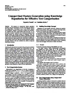
• Wine. This problem, taken from the Irvine Repository, deals with the classification of wines into 3 class types. Each example is represented by 13 continuous attributes, which represent measures of chemical elements in the wine. • Tic-Tac-Toe. The problem, taken from the Irvine Repository, deals with the classification of legal tic-tac-toe end games, as wins or non-wins for the x player. Each example is represented by 9 nominal attributes, which represent the slot values in the range {x, o, b}. • Monks problems. This set of problems, taken from the Irvine Repository, contains the three known monk problems. Each example is represented by 5 nominal attributes in the range {1, 2, 3, 4}. The problems are – (a1 = a2) or (a5 = 1); – exactly two of (a1 = 1, a2 = 1, a3 = 1, a4 = 1, a5 = 1); – ((a5 = 3) and (a4 = 1)) or ((a5 = 4) and (a2 = 3)), with an added 5% class noise. • Attacking queens. The target concept of this problem, illustrated in figure 9, is the existence of a mutual threat between any pair of queens placed on a chess board. In the Queen2 domain, examples are pairs of queens specified by their row and column positions. Similarly, Queen3 deals with triplets of queens. • Soccer offside. This problem, illustrated in figure 9, deals with the classification of soccer field situations as offside or not offside. (An offside situation occurs when a player of one team is placed in front of all the second team’s players, at the moment the ball is being passed ). Each player is represented by two attributes, which describe its X and Y coordinates on the field. We experimented with problems of two 5-player and 11-player teams, expressed by 20 and 44 attributes correspondingly. • Isosceles triangle. This problem, deals with the classification of triangles as isosceles or nonisosceles. Each example triangle is represented by its 3 continuous arc lengths.

Figure 9. The left picture describes the Attacking Queens problem while the right-hand side represents the Soccer Offside problem.

84


Table 1.

Table 2.

The set of all the constructor functions used for the experiments. Standard Mathematical functions

+, −, ÷, ∗, = , AbsDiff , Average, Max, Min.

Standard Logic functions

And, Or

Special Logic functions

Count denoted as Count(b1 , . . . , bn ) returns the number of its Boolean arguments which hold a TRUE value.

Interval functions

Is( f, c) = TRUE ⇔ f = c InRange( f, c1 , c2 ) = TRUE ⇔ f ∈ [c1 , c2 ].

Problems and their supplied constructor functions.

Domain

Constructors

Domain

Constructors

Promoter

{Is, Count}

Wine

{÷, ∗, −, +}

Tic-Tac-Toe

{Is, Count}

Chess Queens

{÷, ∗, −, +, AbsDiff }

Soccer Offside

{÷, ∗, −, +, Max, Min}

Balance

{÷, ∗, −, +, AbsDiff }

Heart Disease

{InRange, Count, And}

Iris

{÷, ∗, Avarage}

Monk Problems

{Is, Count, =, Or}

Isosceles Triangle

{÷, ∗, Count, +, −, =}

Although the target concept is quite simple, concept learning algorithms like C4.5 are unable to produce an effective decision tree for its description. • Balance. This problem, taken from the Irvine Repository, was generated to model psychological experimental results. Each example is classified as having a balance scale tipped to the right, tipped to the left, or balanced. Each example is represented by 4 continuous attributes. • Iris. This problem, taken from the Irvine Repository, deals with the classification of iris plants into 3 classes. Each example is represented by 4 continuous attributes. • Heart. This problem, taken from the Irvine Repository, deals with the classification of patients diagnosed to have suffered a heart attack or not. Each example is represented by 14 attributes, mostly continuous, and few nominal attributes. For each problem, FICUS was supplied with constructor functions relevant to the target concept, as well as irrelevant functions to test the resilience of the algorithm. Table 1 contains the space of all constructor functions used for the experiments described here.2 It √ is easy to add additional mathematical functions such as and a X , logic functions such as XOR and domain-specific functions. These constructor functions are able to express some of the representations that have been discussed, such as recursive Boolean expressions, M-of-N expressions (using the Count function), and simple hyperplanes. Table 2 presents the problem domains together with their associated constructor functions. 7.2.

The performance of FICUS

Our basic experiment tests the performance of FICUS with DT for all the domains. Table 3 compares the performance of DT with the basic features to its performance with the features constructed by FICUS.

85


Table 3. The results obtained for the basic experiment set performed with FICUS. Each number represents the average of 10-fold cross-validation. The numbers in parentheses are confidence intervals for p = 0.95. The table presents both feature quality results expressed by accuracy and tree size, and generation resources represented by CPU seconds, number of evaluated features and estimated complexity. DT

Domain

DT

+ FICUS

Accuracy Size

FICUS

Weighted size

FICUS

Time Evaluated (Seconds) features

Est. comp.

Accuracy

Size

Promoter

73.55 (±5.88)

31.6

83.48 (±4.61)

9.0

14.7

9.94 (±6.69)

9.0

4301

397726

Wine

92.67 (±3.81)

13.9

95.25 (±2.65)

7.4

13.0

2.57 (±4.03)

6.9

1576

964325

TicTacToe

85.38 247.0 (±2.18)

96.45 64.5 (±1.68)

113.7

11.00 (±2.24)

90.9

21625

12562211

Queens2

66.94 337.1 (±4.03)

100.00 (±0.00)

5.0

15.0

33.06 (±4.03)

7.8

1625

2246981

Queens3

66.37 262.1 (±2.58)

98.06 23.2 (±1.64)

40.1

31.69 (±2.65)

40.1

14074

7889049

Offside5

78.71 (±3.47)

86.7

98.55 11.6 (±0.85)

42.1

19.84 (±3.77)

39.2

9755

7747704

Offside11

66.94 (±2.65)

99.5

81.94 62.2 (±3.04)

123.5

15.00 (±4.03)

108.8

36931

22626038

Isosceles

62.10 205.1 (±2.75)

100.00 (±0.00)

3.0

11.0

37.90 (±2.75)

5.5

395

950957

Balance

78.08 222.8 (±2.26)

99.84 (±0.36)

5.0

15.0

21.76 (±2.17)

18.3

5485

4231528

Heart

75.76 (±2.89)

76.8

77.27 67.2 (±1.55)

75.7

1.51 (±3.29)

10.7

6770

1056581

Iris

94.67 (±2.80)

14.6

93.67 (±4.27)

8.4

12.9

−1.00 (±3.90)

3.8

496

180782

Monk1

99.27 116.1 (±0.63)

100.00 (±0.00)

3.0

6.0

0.73 (±0.63)

1.6

276

99538

Monks2

82.74 283.8 (±2.42)

100.00 27.4 (±0.00)

58.8

17.26 (±2.42)

44.0

13418

5880228

Monks3

100.00 143.6 (±0.00)

100.00 (±0.00)

7.0

0.00 (±0.00)

3.8

353

406748

5.0

advantage

resources

The table presents the results achieved by employing a default configuration where Niterations = 2, Nphase = 2, Nnew = 100 and Evaluation Strategy = Hybrid. It is clear that FICUS significantly improved the classification accuracy for most domains. FICUS also achieved better values of standard deviation. This reflects higher stability. FICUS dramatically reduced the size of the produced tree classifiers. It also significantly reduced the weighted tree size for all the problems containing only nominal attributes. For problems containing continuous attributes, the reduction was sometimes less significant, and in a

86


Table 4. A comparison between the performance of FICUS and other feature construction algorithms. Algorithms whose feature representation is believed to be unsuitable for a problem domain were denoted in the table as N/S (not suitable) with respect to the given problem. The numbers in parentheses are standard deviations. FICUS

Problem

DT

+

DT

GALA

+

C4.5

LFC

ID2-of-3 (M-of-N)

Promoter

73.55 (±7.8)

83.48 (±6.1)

79.5 (±7.8)

75.1 (±7.0)

Wine

92.67 (±5.0)

95.25 (±3.5)

93.8 (±3.0)

–

87.6 –

TicTacToe

85.38 (±2.9)

96.45 (±2.2)

–

–

94.9

Queens2

66.94 (±5.3)

100.00 (±0.0)

N/S

N/S

N/S

Queens3

66.37 (±3.4)

98.06 (±2.1)

N/S

N/S

N/S

Offside5

78.71 (±4.6)

98.55 (±1.1)

N/S

N/S

N/S

Offside11

66.94 (±3.5)

81.94 (±4.0)

N/S

N/S

N/S

Isosceles

62.10 (±3.6)

100.00 (±0.0)

N/S

N/S

N/S

Balance

78.08 (±3.0)

99.84 (±0.5)

–

–

–

Heart

75.76 (±3.8)

77.27 (±2.0)

76.4 (±2.5)

75.2 (±2.7)

76.8

Iris

94.67 (±3.7)

93.67 (±5.6)

–

–

–

Monk1

99.27 (±0.8)

100.00 (±0.0)

–

–

100

Monks2

82.74 (±3.2)

100.00 (±0.0)

–

–

98

Monks3

100.00 (±0.0)

100.00 (±0.0)

–

–

97.2

few cases the weighted tree size increased, regardless of the improvement in classification accuracy. Table 4 compares the results achieved by FICUS to those reported for other feature construction algorithms for several UCI problems. Only UCI problems found suitable for these algorithms’ representations were used. The results for ID2-of-3 are taken from (Zheng, 1996). In spite of its generality, the performance of FICUS was found to be comparable, and in most cases superior to that of special-purpose construction algorithms, with respect to their favorable domains. In addition, FICUS was successfully applied to other complex problems such as Attacking Queens and Soccer Offside, for which the algorithms mentioned could not be effectively applied due to their restricted representational power. Algorithms whose feature representation is believed to be unsuitable for a problem domain were denoted in the table as N/S (not suitable) with respect to the given problem. Table 5 presents some of the prominent features that were generated by FICUS when applied to the tested classification problems. The presented features appear in the majority of the classifiers that were generated for the tested problem, mostly in those whose accuracy is high in comparison to the accuracy of classifiers that used the basic features. As can be seen from the table, for the cases where the target concept is known, the prominent features partially (or fully) express the underlying problem concept. Such features enable the concept learner to increase the accuracy, compactness and comprehensibility of the produced classifiers. For example, in the tic-tac-toe domain, almost all the features that were output by FICUS are those using the count constructor to identify full rows, columns and diagonals of the same color. In the promoter domain, FICUS identified the


87

Table 5. A list of prominent features produced by the FICUS algorithm. These examples demonstrate the ability of FICUS to discover features that are strongly related to the target concept. Domain Promoter

Prominent generated feature(s) Count (Is(p-34,G),Is(p-36,T), Is(p-35,T)) This prominently produced feature describes the minus 35 contact region, which has been identified in many recognized promoters.

Offside-11

/(Max(w8 y , w9 y , Max(w1 y , w2 y , w11 y ), Max(w5 y , w6 y , w11 y , Max(w3 y , w4 y , w10 y ))), Max(b4 y , b6 y , b9 y , Max(b1 y , b2 y , b8 y ), Max(b5 y , b7 y , b9 y , Max(b3 y , b10 y , b11 y )))) This complex feature, which appeared in similar versions throughout the produced classifiers, almost fully describes the entire target concept. w6 y is the Y coordinate of player no. 6 of the white team.

Queens-3

*(AbsDiff (Q1x , Q2x ), AbsDiff (Q1 y , Q2 y )), AbsDiff (AbsDiff (Q1x , Q2x ), AbsDiff(Q1 y , Q2 y )) The first feature identifies whether Queens 1 and 2 are placed on the same row or column, while the second feature identifies whether they are placed on any common diagonal. Similar symmetric features identified threats between other queen pairs.

Isosceles

Count(= (A1, A2), = (A2, A3), = (A3, A1)) This feature completely represents the concept of an isosceles triangle, which requires at least one pair of equal arcs.

Tic-Tac-Toe

Count(Is(s1 , x), Is(s2 , x), Is(s3 , x)) Count(Is(s1 , x), Is(s5 , x), Is(s9 , x)) Count(Is(s3 , o), Is(s5 , o), Is(s7 , o)) These representative features describe rows, columns, and diagonals of consecutive x or o signs. Although FICUS was able to produce features of much higher complexity, it almost exclusively produced rows, columns and diagonals of slot triplets.

Monk2

Count(Is(A1 , 1), Is(A2 , 1), Is(A3 , 1), Is(A4 , 1), Is(A5 , 1)) Fully describes the target concept of the Monk2 problem

Wine

∗(Attrib11 , /(Attrib7 , Attrib10 )) This feature and its mathematical equivalents appeared in the majority of classifiers which achieved 100% accuracy. We do not know the meaning of this feature since the wine domain theory was not available to us.

Heart

Count(In Range(cp, −∞, 3.5), In Range(ca, −∞, 0.5) In Range(cp, −∞, 3.5) was a component of most prominent features.

Balance

/(/(Distanceright , Distanceleft ), /(Weightleft , Weightright )) ∗(Distanceright , /(Weightright , ∗(Weightleft , Distanceleft ))) These features fully describe the target concept.

minus 35 contact region, which is considered to be a good promoter indicator by the existing theory. 7.3.

The effect of the number of constructors on the performance of FICUS

Any concept learning task involves a knowledge engineering stage where the expert decides what features will be used for the induction task. Robust learners are able to overcome the

88


Table 6. The results of testing FICUS under two conditions. The third column shows the performance of FICUS when selecting from the union of all the constructor functions of the different domains. The fourth column shows the performance of FICUS with generated features evaluated at the root of the tree only. The numbers in parentheses are confidence intervals for p = 0.95. Domain

DT

DT

+ FICUS

All constructors

Root only

Promoter

73.55 (±5.88)

83.48 (±4.61)

82.03 (±6.00)

83.44 (±6.11)

TicTacToe

85.38 (±2.18)

96.45 (±1.68)

95.36 (±1.34)

88.36 ( ± 2.13)

Queens3

66.37 (±2.58)

98.06 (±1.64)

88.23 (±4.88)

70.32 (±3.66)

Offside5

78.71 (±3.47)

98.55 (±0.85)

97.10 (±2.45)

82.42 (±3.28)

Monks2

82.74 (±2.42)

100.00 (±0.00)

99.92 (±0.18)

92.98 (±3.20)

existence of redundant and irrelevant features. In the FICUS framework, we face a similar situation with the constructors. The expert supplies constructors that are estimated to be relevant to the problem. We tested the robustness of FICUS by giving it the merged set of 5 domains. Table 6 shows the results obtained. We can see that except for one domain, the penalty in performance is negligible. This indicates that FICUS indeed is able to select the right constructors for the generation of good features. 7.4.

The effect of local evaluation on the FICUS

One of the important elements of FICUS is the use of decision trees in order to evaluate features in a local context. We decided to test the utility of this element by turning it off and test the algorithm’s performance. Table 6 shows the results obtained by evaluating features only at the root level of the tree (which is equivalent to not using the tree at all). We can see that in 4 out of the 5 domains the performance of FICUS indeed deteriorated as expected. 7.5.

The effect of the numeric parameters on the performance of FICUS

We have performed several experiments to test the effect of the independent variables described above on the performance of FICUS. We used four problem domains for these experiments: promoter, offside11, 3queens and tic-tac-toe, which represent a variety of domains and learned concepts. The graphs in figure 10 show the mutual effect of the number of iterations (Niterations ) and number of generation-phases (Nphase ) on the accuracy of the produced classifier. As expected, the utility of the generated features increases with the increase in the number of iterations and the number of phases. We found, however, that further increasing the number of generation phases caused an abrupt increase of the feature complexity. The reason for this phenomenon is data overfitting that occurs in tree nodes that contain relatively few cases. In such nodes there is a better chance for generating overly complex

Figure 10.

The mutual effect of the number of iterations & phases on the classification accuracy.


89

90


features that successfully discriminate between members of the two classes in the (relatively small) local instance set. We have indeed witnessed this in several experiments. A possible solution may be to alter the existing evaluation criteria such that the importance of low complexity increases with reverse proportion to the size of the local instance set. For example, in the data-driven evaluation function, h db ( f ), the constant α could be replaced with a function that depends on the size of the local instance set E. Another possible solution for the described phenomenon is pruning. The graphs in figure 11 show the performance of FICUS as a function of its number of evaluated features at each generation phase (Nnew ). These figures also show the effect of the evaluation strategy of building blocks employed by the generator on the achieved performance. Each figure contains two graphs, corresponding to the employed selection strategy. For the offside11 and queens3 problems, which represent complex target concepts, the graphs indicate a noticeable improvement in accuracy as a result of increasing the number of evaluated features. The tic-tac-toe problem demonstrated minimal sensitivity to the number of evaluated features, especially when employing a hybrid selection strategy. For the promoter problem, the optimal number of evaluated features was interestingly discovered to be approximately 12, regardless of the selection strategy. This may result from its large number of irrelevant basic features. This, combined with a small data set, might lead to the construction and selection of superfluous features. The graphs do not indicate a conclusive advantage to either one of the selection strategies, excluding the complex offside11 problem, in which the hybrid strategy significantly outperformed the data-driven. In addition, the hybrid selection strategy outperformed the data-driven when employing a small number (Nnew = 1, . . . , 10) of evaluated features. 7.6.

The performance of FICUS with other concept learners

While FICUS uses DT as an internal procedure for determining local context, the resulting features can be used with other concept learning algorithms. We tested the effect of adding the generated features to the perceptron, back propagation, nearest neighbor and k-nearest neighbor algorithms. Tables 7–12 show the results obtained. We can see from the results that for several domains the performance of the tested algorithm improves significantly when using the features generated by FICUS. For two domains (Isosceles and Monk1), the accuracy obtained by the perceptron algorithm was doubled. For two additional domains (Wine and Monk3) the accuracy improved by more than 20%. The performance of the back propagation algorithm was also improved by the features generated by FICUS, but to a lesser extent. This is not surprising, since we can view the nodes in the hidden layer as intermediate features generated by the back propagation algorithm. Still, for two domains, the difference in accuracy was over 30% in favor of the FICUS enhanced version. For two other domains the difference was around 20%. The performance of all the nearest neighbor classifiers was also significantly improved when using the FICUS generated features. This was achieved despite the sensitivity of nearest neighbor classifiers to redundant features.

Figure 11.

The effect of the number of evaluated features and evaluation strategy on the achieved classification accuracy.


91

92


Table 7. The performance of the perceptron algorithm with the basic features compared to its performance with the featur generated by FICUS. The numbers in parentheses are confidence intervals with p = 0.95. Perceptron

Perceptron + FICUS

Promoter

76.34 (±6.71)

83.96 (±6.22)

7.62 (±8.21)

Wine

30.87 (±5.99)

52.25 (±9.08)

21.39 (±9.52)

TicTacToe

34.66 (±1.84)

37.69 (±3.98)

3.03 (±2.35)

Queens2

58.55 (±4.86)

65.48 (±3.03)

6.94 (±5.00)

Offside5

57.66 (±4.03)

66.13 (±6.77)

8.47 (±6.83)

Offside11

55.48 (±4.14)

60.32 (±7.36)

4.84 (±8.85)

Isosceles

48.70 (±4.73)

98.70 (±1.69)

50.00 (±5.69)

Balance

35.44 (±7.03)

38.80 (±5.09)

3.36 (±6.06)

Heart

62.95 (±7.09)

60.10 (±4.64)

−2.86(±4.53)

Iris

63.33 (±8.63)

66.67 (±5.84)

3.33 (±4.50)

Monk1

49.35 (±2.65)

100.00 (±0.00)

50.65 (±2.65)

Monk2

48.79 (±6.55)

55.97 (±8.30)

7.18 (±9.66)

Monk3

75.97 (±2.85)

98.79 (±1.34)

22.82 (±3.61)

Domain

Difference

Table 8. The performance of the back propagation algorithm with the basic features compared to its performance with the features generated by FICUS. The numbers in parentheses are confidence intervals with p = 0.95. Backprop

Backprop + FICUS

Difference

Promoter

82.49 (±6.45)

83.42 (±7.73)

0.93 (±3.86)

Wine

89.63 (±6.61)

90.79 (±7.31)

1.16 (±2.73)

TicTacToe

62.90 (±3.88)

81.66 (±14.46)

18.76 (±16.08)

Queens2

72.98 (±5.05)

96.13 (±3.38)

23.15 (±6.00)

Offside5

68.23 (±3.51)

75.73 (±4.97)

7.50 (±3.63)

Offside11

59.52 (±3.76)

65.00 (±5.30)

5.48 (±4.79)

Isosceles

61.50 (±3.17)

92.60 (±11.16)

31.10 (±11.78)

Balance

86.40 (±2.27)

89.44 (±3.61)

3.04 (±2.88)

Heart

76.93 (±1.93)

77.10 (±3.25)

0.17 (±4.17)

Iris

85.00 (±4.93)

84.67 (±5.05)

−0.33(±1.35)

Monk1

93.87 (±6.65)

100.00 (±0.00)

6.13 (±6.65)

Monk2

65.16 (±4.48)

99.27 (±0.84)

34.11 (±4.63)

Monk3

97.74 (±1.08)

97.58 (±1.02)

−0.16(±0.76)

Domain

8.

Discussion

We presented the FICUS construction algorithm, which receives the standard input of supervised learning, as well as a feature representation specification (FSS), and uses them to produce a set of generated features. FICUS searches its defined feature space, continuously attempting to improve its generated feature set as long as resources are available. The


93

Table 9. The performance of the nearest neighbor algorithm with the basic features, compared to its performance with the features generated by FICUS. The numbers in parentheses are confidence intervals with p = 0.95. Nearest

Nearest + FICUS

Difference

Promoter

77.73 (±6.91)

82.01 (±4.84)

4.29 (±4.67)

Wine

96.63 (±1.59)

97.47 (±1.49)

0.84 (±1.89)

TicTacToe

67.43 (±1.69)

94.73 (±2.11)

27.30 (±1.75)

Queens2

70.81 (±2.77)

86.21 (±1.97)

15.40 (±2.11)

Offside5

59.35 (±1.54)

67.58 (±4.14)

8.23 (±4.39)

Offside11

54.19 (±2.90)

58.55 (±4.36)

4.35 (±4.96)

Isosceles

69.20 (±1.25)

100.00 (±0.00)

30.80 (±1.25)

Balance

56.56 (±2.98)

79.52 (±3.99)

22.96 (±4.55)

Heart

76.43 (±2.28)

77.10 (±3.11)

0.68 (±4.07)

Iris

94.00 (±4.32)

94.00 (±4.18)

0.00 (±1.59)

Monk1

88.31 (±1.77)

100.00 (±0.00)

11.69 (±1.77)

Monk2

87.98 (±2.01)

100.00 (±0.00)

12.02 (±2.01)

Monk3

91.94 (±2.12)

100.00 (±0.00)

8.06 (±2.12)

Domain

Table 10. The performance of the 3-nearest neighbor algorithm with the basic features, compared to its performance with the features generated by FICUS. The numbers in parentheses are confidence intervals with p = 0.95. 3-Nearest

3-Nearest + FICUS

Promoter

79.18 (±6.32)

86.30 (±4.96)

Wine

96.35 (±1.67)

97.47 (±1.49)

1.12 (±1.39)

TicTacToe

67.95 (±1.82)

96.14 (±2.03)

28.19 (±1.82)

Queens2

70.81 (±2.09)

82.98 (±2.27)

12.18 (±2.64)

Offside5

63.79 (±2.61)

72.58 (±4.19)

8.79 (±3.29)

Offside11

52.66 (±2.67)

60.89 (±3.94)

8.23 (±4.16)

Isosceles

66.70 (±2.52)

100.00 (±0.00)

33.30 (±2.52)

Balance

68.00 (±2.53)

80.96 (±2.70)

12.96 (±2.45)

Heart

80.15 (±3.01)

78.46 (±1.61)

−1.69 (±2.60)

Iris

94.67 (±3.59)

94.33 (±3.56)

−0.33 (±0.75)

Monk1

81.85 (±2.67)

99.35 (±0.65)

17.50 (±2.73)

Monk2

76.13 (±2.96)

99.92 (±0.18)

23.79 (±2.97)

Monk3

92.02 (±2.08)

99.92 (±0.18)

7.90 (±1.96)

Domain

Difference 7.12 (±3.69)

algorithm bases its operation on the framework of decision tree learning, which defines its feature construction context. The algorithm uses general construction operators whose actual action is determined by the input FSS. It also uses general feature evaluation functions that can be uniformly applied to different forms of constructed features. Both data-driven and hypothesis-driven strategies are employed by the algorithm to guide its conducted search.

94


Table 11. The performance of the 5-nearest neighbor algorithm with the basic features, compared to its performance with the features generated by FICUS. The numbers in parentheses are confidence intervals with p = 0.95. Domain

5-Nearest

5-Nearest + FICUS

Difference 9.05 (±5.17)

Promoter

76.84 (±8.26)

85.89 (±6.34)

Wine

96.35 (±0.97)

97.18 (±1.89)

0.83 (±2.12)

TicTacToe

70.41 (±1.82)

95.35 (±1.91)

24.95 (±2.02)

Queens2

71.94 (±1.86)

84.84 (±1.94)

12.90 (±1.92)

Offside5

66.94 (±2.26)

75.81 (±3.73)

8.87 (±2.94)

Offside11

55.16 (±4.14)

62.74 (±4.85)

7.58 (±3.55)

Isosceles

64.50 (±2.27)

100.00 (±0.00)

35.50 (±2.27)

Balance

74.16 (±2.06)

82.56 (±4.22)

8.40 (±3.39)

Heart

81.16 (±3.26)

81.49 (±2.10)

0.32 (±2.26)

Iris

95.00 (±3.03)

94.67 (±3.02)

−0.33(±0.75)

Monk1

78.63 (±2.21)

98.63 (±0.72)

20.00 (±1.80)

Monk2

71.29 (±4.43)

99.52 (±0.49)

28.23 (±4.44)

Monk3

93.31 (±2.09)

99.35 (±0.65)

6.05 (±2.06)

Table 12. The performance of the 7-nearest neighbor algorithm with the basic features, compared to its performance with the features generated by FICUS. The numbers in parenthesis are confidence intervals with p = 0.95. 7-Nearest

7-Nearest + FICUS

Difference

Promoter

75.43 (±6.20)

85.43 (±5.54)

10.00 (±5.87)

Wine

96.90 (±2.02)

97.46 (±1.99)

0.56 (±2.28)

TicTacToe

76.36 (±1.87)

94.99 (±1.69)

18.63 (±2.15)

Queens2

71.53 (±3.41)

86.13 (±1.65)

14.60 (±2.86)

Offside5

66.29 (±2.96)

75.89 (±4.30)

9.60 (±3.54)

Offside11

56.05 (±3.66)

63.87 (±6.18)

7.82 (±4.41)

Isosceles

61.90 (±2.56)

100.00 (±0.00)

38.10 (±2.56)

Balance

77.68 (±1.33)

83.84 (±4.07)

6.16 (±3.62)

Heart

80.99 (±2.20)

83.68 (±2.92)

2.69 (±2.20)

Iris

94.67 (±3.02)

95.00 (±2.81)

0.33 (±0.75)

Monk1

78.55 (±2.04)

98.31 (±0.69)

19.76 (±1.91)

Monk2

67.58 (±2.14)

99.84 (±0.36)

32.26 (±2.21)

Monk3

93.55 (±1.90)

99.11 (±0.63)

5.56 (±1.73)

Domain

While FICUS is similar in some aspects to some of the existing feature construction algorithms (such as LFC, CITRE, GALA, and FRINGE), its main strength and contribution are its generality and flexibility. FICUS was designed to perform feature generation given any feature representation specification complying to its general purpose grammar (presented in figure 2).


95

The large majority of previous related work presented algorithms for searching some known feature space (such as Boolean expressions, M of N expressions, hyper planes, or bit strings). The novelty of this work is in building an algorithm that searches any member of an infinite family of feature spaces defined by a general purpose grammar. The flexibility of FICUS makes it suitable for a wide variety of feature representations and problem domains. It also enables the use of FICUS to evaluate and discover good feature representations for a given domain. By accepting feature representation as dynamic input, FICUS enables easy incorporation of human domain knowledge. The choice of feature representation (mainly the set of constructor functions) is up to the deployer of FICUS. As in the general case of concept learning, poor representation leads to poor results. In our experiments, FICUS performed very well with relatively simple sets of constructor functions that seemed potentially relevant to the given domain. In a lesion study, we supplied FICUS with the union of constructor sets of the individual domains. The results showed only minor deterioration in FICUS’s performance, indicating its robustness to irrelevant constructors. The deterioration that did occur as a result of using irrelevant constructor functions is analogous to the existing findings (Kira & Rendell, 1992; John, Kohavi & Pfleger, 1994; Kohavi & Dan, 1995; Sangiovanni-Vincentelli, 1992; Caruana & Freitag, 1994; Salzberg, 1993) regarding the use of irrelevant attributes in classical concept learning. In both cases, deterioration in accuracy is caused by the data overfitting that results from increasing the feature space. An interesting direction for overcoming this problem could be to exploit the fact that FICUS receives its representation language as dynamic input for conducting a search in the representation space. Methods similar to those employed for feature selection (John, Kohavi, & Pfleger, 1994; Kohavi & Dan, 1995; Salzberg, 1993) could be adopted to find a utile subset of constructor functions. FICUS employs the decision tree algorithm DT as an internal mechanism for directing feature construction. The decision tree splits the instance space into exclusive subspaces for which feature construction is locally applied. Performing local feature construction for different subspaces of the instance space has proved effective especially for complex and disjunctive concepts. A lesion study in which feature construction was performed only for the entire instance space (only at the root of the tree) showed significant deterioration in performance. The internal decision tree algorithm is a straightforward implementation of ID3 without pruning or other advanced improvements. We would like to explore the effect of adding pruning to the internal concept learner (DT). It is quite possible that pruning would remove subtrees with irrelevant constructed features, thus improving the quality of the set of constructed features passed to the next iteration. Regardless of the fact that the DT algorithm is used internally, the output of FICUS is a feature set, and not the final decision tree built in the last iteration. Therefore, FICUS can be used in conjunction with concept learners other than DT. Our experiments showed significant improvement for all tested concept learners, including perceptron, back propagation, and nearest neighbor. It is interesting to view the FICUS algorithm as an evolutionary process. The population is the set of constructed features. New members of the population are constructed by combining existing feature pairs of high fitness. The fitness is assigned by the building block

96


evaluation functions, which look at properties such as information gain, complexity and relative gain with respect to the parents. The pairs are combined by applying a set of predefined combination operators (Compose, Insert, Replace and Interval). The population is kept at a fixed size by removing members with low fitness. The particular tree-based representation used by FICUS resembles the tree-structured elements manipulated by genetic programming algorithms (Koza, 1992; Koza et al., 1996). The merit of our approach was demonstrated by applying the algorithm to various classification problems. FICUS was able to significantly improve the accuracy of the resulting classifiers for several types of concept learners. In addition, it generated features that often expressed important aspects of the underlying target concept. FICUS’s general and flexible form of feature representation turns it into an effective tool for discovering useful representations with respect to a given classification problem. It also enables utilization of partial domain-specific human knowledge for this purpose. One limitation of the FICUS framework is that its search algorithm depends on the assumption that building blocks of complex features of high utility will also be found to be utile. While this was the case in most of the problems upon which FICUS was tested, it is quite possible that in certain domains this assumption does not hold and a gradual generation of structured features will not be effective. This problem may be addressed by increasing the beam size of the search algorithm. Such an increase, however, is quite restricted due to its high computational demands. FICUS runs as a preprocessing stage, prior to to concept learning. Therefore, its nontrivial resource requirement is added to the overall execution time. This might seem to limit our approach. Nevertheless, the user can control the amount of resources invested in feature generation. Therefore, the combined system can be viewed as an anytime concept learning algorithm. That means that the user can specify the required tradeoff between learning resources and expected classification accuracy. As can be seen in our experiments, investing an additional several seconds can yield a very significant improvement in accuracy. To conclude, many researchers have shown the benefit of feature generation for solving classification problems. Many alternative feature generation algorithms based on a variety of representation schemes have been proposed. The methodology presented here offers a general framework for feature generation and has several advantages over existing algorithms. While other algorithms are tailored to a predefined feature representation that may not be inappropriate for the problem at hand, the FICUS algorithm allows a flexible representation which may appropriate for a variety of domains. The most important advantage of our framework is that it allows expressing and exploiting partial background knowledge for constructing utile features. Such knowledge is commonly available for real-world problems, but can not be easily exploited by other feature generation algorithms due to their representational rigidity.

Notes 1. Feature Incremental ConstrUction System. 2. The AbsDiff function measures the absolute difference between two numeric values.


97

References Aha, D. W. (1991). Incremental constructive induction: An instance-based approach. In Proc. 8th International Conference on Machine Learning (pp. 117–121). San Mateo, CA: Morgan Kaufmann. Aha, D. W., Kibler, D., & Albert, M. K. (1991). Instance-based learning algorithms. Machine Learning, 6, 37–66. Bala, J. W., Michalski, R., & Wenk, J. (1992). The principal axes method for constructive induction. In Proc. 9th International Conference on Machine Learning (pp. 20–29). San Mateo, CA: Morgan Kaufmann. Boddy, M. (1991). Anytime problem solving using dynamic programming. In Proceedings of the Ninth National Conference on Artificial Intelligence (Vol. II, pp. 738–743). Menlo Park: AAAI Press/MIT Press. Boddy, M., & Dean, T. (1994). Decision-theoretic deliberation scheduling for problem solving in time-constrained environments. Artificial Intelligence, 67:2, 245–286. Breiman, L., Friedman, J., Olshen, R., & Stone, C. (1984). Classification and Regression Trees. Belmont: CA Wadsworth International Group. Caruana, R., & Freitag, D. (1994). Greedy attribute selection. In Proc. 11th International Conference on Machine Learning (pp. 28–36). San Mateo, CA: Morgan Kaufmann. Clark, P., & Niblett, T. (1989). The cn2 induction algorithm Machine Learning, 3, 261–283. De Jong, K. A., Spears, W. M., & Gordon, D. F. (1992). Using genetic algorithms for concept learning. Machine Learning, 8, 5–32. Fayyad, U., & Irani, K. (1993). Multi-interval discretization of continuous-valued attributes for classifition learning. In Proc. 13th International Conference on Artificial Intelligence (pp. 1022–1027). Heath, D., Kasif, S., & Salzberg, S. (1993). Learning oblique decision trees. In Proc. 13th International Conference on Artificial Intelligence (pp. 1003–1007). Hirsh, H., & Japkowicz, N. (1994). Bootstrapping training-data representations for inductive learning: A case study in molecular biology. In Proc. 11th International Conference on Machine Learning (pp. 639–644). San Mateo, CA: Morgan Kaufmann. Hu, Y.-J., & Kibler, D. (1996). Generation of attributes for learning algorithms. In Proc. 13th International Conference on Machine Learning. San Mateo, CA: Morgan Kaufmann. Ittner, A., & Schlosser, M. (1996). Discovery of relevant new features by generating non-linear decision trees. In Proc. 2nd International Conference on Knowledge Discovery and Data Mining (KDD’96). John, G. H., Kohavi, R., & Pfleger, K. (1994). Irrelevant features and subset selection problem. In Proc. 11th International Conference on Machine Learning (pp. 121–129). San Mateo, CA: Morgan Kaufmann. Kira, K., & Rendell, L. A. (1992). A practical approach to feature selection. In Proc. 9th International Conference on Machine Learning (pp. 249–256). San Mateo, CA: Morgan Kaufmann. Kohavi, R., & Dan, S. (1995). Feature subset selection using the wrapper model: Overfitting and dynamic search space topology. In U. M. Fayyad and R. Uthurusamy (Eds.), First International Conference on Knowledge Discovery and Data Mining (KDD-95). Koza, J. (1992). Genetic programming: On the programming of computers by means of natural selection. Master’s thesis. Cambirdge, MA: MIT Press. Koza, J. R., Bennett, F. H., Andre, D., & Kean, M. A. (1996). Four problems for which a computer program evolved by genetic programming is competitive with human performance. In Proceedings of the 1996 IEEE International Conference on Evolutionary Computation (pp. 1–10). Piscataway, NJ: IEEE Press. Matheus, C. J., & Rendell, L. A. (1989). Constructive induction on decision trees. In Proc. 11th International Conference on Artificial Intelligence (pp. 645–650). Murphy, P. M., & Pazzani, M. J. (1991). Id2-of-3: Constructive induction of m-of-n concepts for discriminators in decision trees. In Proc. 8th International Conference on Machine Learning (pp. 183–188). San Mateo, CA: Morgan Kaufmann. Pagallo, G., & Haussler, D. (1990). Boolean feature discovery in empirical learning. In Proc. 7th International Conference on Machine Learning (pp. 71–99). San Mateo, CA: Morgan Kaufmann. Perez, E., & Rendell, L. A. (1995). Using multidimensional projection to find relations. In Proc. 14th International Conference on Artificial Intelligence (pp. 447–455). Quinlan, J. R. (1993). C4.5: Programs for Machine Learning. San Mateo, CA: Morgan Kaufmann.

98


Ragavan, H., & Rendell, L. A. (1993). Improving the design of induction methods by analyzing algorithm functionality and data-based concept complexity. In Proc. 13th International Conference on Artificial Intelligence (pp. 952–958). Ragavan, H., Rendell, L. A., Shaw, M., & Tessmer, A. (1993). Complex concept acquisition through directed search and feature caching. In Proc. 13th International Conference on Artificial Intelligence (pp. 946–951). Salzberg, S. (1993). Improving classification methods via feature selection. Machine Learning, 99. Sangiovanni-Vincentelli, A. L. O. A. (1992). Constructive induction using a non-greedy strategy for feature selection. In Proc. 9th International Conference on Machine Learning (pp. 355–360). San Mateo, CA: Morgan Kaufmann. Schlimner, J. (1987). Concept acquisition through representational adjustment. Ph.D. Thesis, Department of Information and Computer Science, University of California, Irvine, CA. Sutton, R. S., & Matheus, C. J. (1991). Learning polynomial functions by feature construction. In Proc. 8th International Conference on Machine Learning (pp. 208–212). San Mateo, CA: Morgan Kaufmann. Todorovski, L., & Dzeroski, S. (1997). Declarative bias in equation discovery. In Proc. 14th International Conference on Machine Learning. San Mateo, CA: Morgan Kaufmann. Utgoff, P. E., & Brodley, C. E. (1991). Linear machine decision trees. Tech. rep., COINS Technical Report 91–10. Watanabe, L., & Rendell, L. A. (1991). Feature construction in structural decision trees. In Proc. 8th International Conference on Machine Learning (pp. 218–222). San Mateo, CA: Morgan Kaufmann. Wenk, J., & Michalski, R. S. (1994). Hypothesis-driven constructive induction in aq17-hci: A method and experiments. Machine Learning, 14, 139–168. Yang, D.-S., Rendell, L. A., & Blix, G. (1991). Fringe-like feature construction: A comparative study and a unifying scheme. In Proc. 8th International Conference on Machine Learning (pp. 223–227). San Mateo, CA: Morgan Kaufmann. Zheng, Z. (1996). Constructing nominal x-of-n attributes. In Proc. 13th International Conference on Machine Learning (pp. 1064–1070). San Mateo, CA: Morgan Kaufmann. Received May 28, 1998 Revised April 10, 2001 Accepted April 11, 2001 Final manuscript August 20, 2001

Feature Generation Using General Constructor Functions - Springer Link

Feature Generation Using General Constructor Functions - Springer Link

Suggest Documents

Facial Feature Extraction Using Geometric Feature and ... - Springer Link

Conditional Image Generation using Feature

feature article - Springer Link

feature article - Springer Link

feature article - Springer Link

feature article - Springer Link

feature article - Springer Link

feature article - Springer Link

feature article - Springer Link

Feature Selection Using Fuzzy Objective Functions - CiteSeerX

The Constructor: a web application optimizing cloning ... - Springer Link

constructor - Associated General Contractors of California

constructor - Associated General Contractors of California

Feature Generation for Text Categorization Using

Feature Generation Using Genetic Programming With ... - CiteSeerX

Unsupervised Feature Generation using ... - Semantic Scholar

CMR right ventricular strain assessment using feature ... - Springer Link

Learning Hash Functions Using Column Generation

3D motion matching algorithm using signature feature ... - Springer Link

Using Stepwise Feature Introduction in Practice - Springer Link

Feature Extraction Using Pitch Class Profile ... - Springer Link

Joint feature re-extraction and classification using an ... - Springer Link

Using Non-Feature Films to Teach Diversity, Cultural ... - Springer Link

3D motion matching algorithm using signature feature ... - Springer Link