To improve computer aided diagnosis (CAD) for CT colonography we designed a hybrid classification scheme that uses a committee of support vector machines ...
Feature Selection for Computer-Aided Polyp Detection using Genetic Algorithms Meghan T. Miller1, Anna K. Jerebko1, James D. Malley2, Ronald M. Summers1 1 2
Clinical Center, Department of Diagnostic Radiology, NIH Center for Information Technology, NIH.
ABSTRACT To improve computer aided diagnosis (CAD) for CT colonography we designed a hybrid classification scheme that uses a committee of support vector machines (SVMs) combined with a genetic algorithm (GA) for variable selection. The genetic algorithm selects subsets of four features, which are later combined to form a committee, with majority vote for classification across the base classifiers. Cross validation was used to predict the accuracy (sensitivity, specificity, and combined accuracy) of each base classifier SVM. As a comparison for GA, we analyzed a popular approach to feature selection called forward stepwise search (FSS). We conclude that genetic algorithms are effective in comparison to the forward search procedure when used in conjunction with a committee of support vector machine classifiers for the purpose of colonic polyp identification. Key Words: genetic algorithms, support vector machines, feature selection, forward stepwise search, computer aided diagnosis, virtual colonoscopy.
1. INTRODUCTION 1.1 Computer Aided Diagnosis Colon cancer is the second leading cause of cancer deaths in the US, and research for the development of computer aided procedures for screening patients for colonic carcinoma has grown as a result of the recognized disadvantages that accompany the current standard procedure, the colonoscopy. Computer aided diagnosis (CAD) combined with computed tomographic (CT) colonography, is an alternative. In order for an alternative screening procedure to prevail it must be both sensitive and specific. There is an ongoing effort by several institutions to develop classification schemes that optimize the performance of CAD methods for colon polyp detection. Summers et al. [1] describes recent work on a version of computer automated polyp detection that uses geometric and volumetric features, acquired from the CT data, as the basis for polyp identification. The software first segments the colon using a region growing algorithm, after which, regions of interest along the colon wall are identified. A total of 80 different quantitative features are currently calculated for each polyp candidate, but not all these features are eventually useful. Classification of the candidates is provided by a committee of trained support vector machines (SVMs), each of which uses a four feature input vector. 1.2 Polyp Classification An essential reference for classification, statistical learning machines, and support vector machines (SVMs) in particular, is Hastie et al. [2]. Additional material can be found in Cristianini & Shawe-Taylor [3] and Schölkopf et al. [4]. Consider first constructing an SVM based on the original data,
102
Medical Imaging 2003: Physiology and Function: Methods, Systems, and Applications, Anne V. Clough, Amir A. Amini, Editors, Proceedings of SPIE Vol. 5031 (2003) © 2003 SPIE · 1605-7422/03/$15.00
which consists of N pairs (x1 , y1 ),(x 2 , y2 ),...,(x N , y N ) , for p-dimensional features (predictors) xi ∈ ℜ p and outcomes (polyp, nonpolyp) yi ∈ {+1,−1}.
Define a linear decision boundary (hyperplane) by
{x : f (x) = x T β + β0 = 0}, where β is a unit vector β = 1. One can define a classification rule based on f(x) through G(x) = sign[ f (x)] such that for the test pair (x,y), the observation y is declared a polyp if G(x) > 0, and a non-polyp if G(x) ≤ 0. We observe that f(x) is the signed distance from the data point x to the hyperplane defined by f(x) = 0. We define the margin, C, for the SVM to be 2C = 2 / β . To place the SVM scheme in a larger context, we note that the optimization problem can be restated as a penalized likelihood problem, such that f (x) = x T β + β 0 solves the problem N min β ,β ∑i=1 [1− yi f (x i )]+ + λ β , 2
0
where λ = 1/2γ , and the subscript “+” denotes the positive part of the function. This has the general form of loss function + penalty function.
The optimization problem also has an elegant statement in terms of reproducing kernel Hilbert spaces ([2]; pp. 377-384), and the mathematics of the subject is rich and well-studied. In this context the penalty function above can be generalized, and many choices are then available for the kernel K, among which are polynomials of user-specified degree d, radial basis functions, or weighted hyperbolic tangents (so-called neural network kernels). Using alternative loss functions leads to different classification schemes: the binomial log-likelihood generates the logistic regression scheme, and squared-error loss leads to a penalized linear discriminant decision engine [2]. An important further extension of the SVM architecture is through the use of functions, h j ( x ), j = 1, 2, . . . , M, of the original data vector x. It is possible that such functions transform the problem into a nearly linear one in a sufficiently high dimensional space, and thus that the decision boundary can be easily found. We chose to use degree two polynomial functions of the data, thereby using quadratic kernels in the algorithm.
1.3 Feature Selection
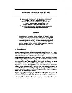
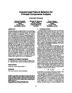
Pattern recognition relies on the extraction and selection of features that adequately characterize the objects of interest. The task of identifying the features that perform well in a classification algorithm is a difficult one, and the optimal choice can be non-intuitive; features that perform poorly separately can often prevail when paired with other features. The filter approach to feature selection tries to infer which features will work well for the classification algorithm by drawing conclusions from the observed distributions (histograms) of the individual features. However, here we see that the histograms give little insight into the separation between polyps and non-polyps. In Figure 1, are the histograms of four features that nonetheless combine to form a good classifier. Clearly the correlation structure of the data is responsible for the success of the joint classifier, and a good classification scheme will attempt to utilize this structure.
Proc. of SPIE Vol. 5031
103
_____________________________________________________________________________________
Polyps
(a) Maximum Average Neck Curvature (cm-1)
(c) Volume (cc)
Nonpolyps
(b) Wall Thickness (cm)
(d) Average Volumetric Gaussian Curvature (cm-2)
Figure 1 Histogram plots showing the frequency of polyps (black) and nonpolyps(white) for four features. Together these four features perform well when used jointly in the support vector classifier, but individually provide no information regarding separation. ___________________________________________________________________________________
Another technique, known as wrapper feature selection [5], uses the method of classification itself to measure the importance of a feature or feature set. The goal in this approach is maximizing the predicted classification accuracy. This approach, while more computationally expensive, tends to provide better results than the simpler filter methods [6]. Recent work in the field of pattern recognition explores the use of evolutionary algorithms for feature selection [7,8,6,9,10,11], and genetic algorithms (GAs)are one type of evolutionary algorithm that can be used effectively as engines for solving the feature selection problem. Feature selection using genetic algorithms has been studied and proven effective in conjunction with various classifiers, including knearest neighbors, and neural networks [8,9,12]. For the research of colonic polyp recognition, with its continually growing list of possible features, it is important to have an efficient and robust feature selection algorithm. The objective of this study is to determine if GA offers a practical approach to feature selection for our data and classification techniques. We compare the results obtained by GA with a forward stepwise selection (FSS) algorithm. 104
Proc. of SPIE Vol. 5031
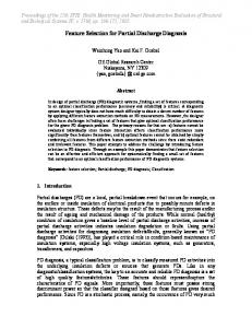
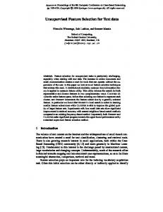
2. METHODS 2.1 Genetic Algorithms GAs are designed to simulate the evolutionary processes that occur in nature [11,13]. The basic idea is derived from the Darwinian theory of survival of the fittest. Three fundamental mechanisms drive the evolutionary process: selection, crossover and mutation within chromosomes. As in nature, each mechanism occurs with a certain probability, allowing for some randomness. Selection occurs on the current population by choosing the most-fit individuals to reproduce. Reproduction, then, can result in the crossover and/or mutation of parent genes to form new solutions. The ratio of heuristic and stochastic decisions, at best, creates a natural balance between survival and evolution. For each generation of the GA, individual solutions are evaluated using a fitness function. The evaluation method is a very important component of the selection process since offspring for the next generation are determined by the fitness values of the present population. Figure 2 provides a simple diagram of the iterative nature of genetic algorithms. The generational process ends when the user defined goal is reached. In most cases, the number of generations is a constant set by the user.
There is some variability introduced by the probability parameters and functions associated with GAs. Function variations range from initialization techniques to additional evolutionary functions. Efforts directed toward analyzing the effects of parameter variation give us some insight into the types of parameter settings that work best in certain situations [14]. The parameters for the designed GA, including population size, probability of crossover and mutation, and selection strategy, were determined manually (Table 1). The major design components of the GA include the initialization process, the design of the evolutionary functions, and an objective fitness function. Initialization: Conventional feature selection allows for variability of both the features and the size of the feature vector. However, the search space can be reduced by using heuristics and/or constraints that accompany the problem [5]. It has generally been observed that when more features are used for classification, more training samples are needed [15]. Our data set, while one of the largest of its kind, still consists of a relatively small number of training samples. Through our experience it was determined that the SVMs functioned well with sets of four features. We held the feature set size constant to effectively reduce the search space and increase the computational efficiency of the genetic algorithm. 100 chromosomes were initialized by random variable selection, and were encoded as four digit integer vectors.
INITIAL POPULATION
EVALUATE
SELECTION
CROSSOVER
MUTATION
Figure 2 Flow diagram depicting the evolutionary process that a genetic algorithm follows.
Population Size Tournament Selection Size Probability of Crossover Probability of Mutation Number of Generation
100 10 0.90 0.10 20
Table 1. A list of the parameter settings used for the GA
Proc. of SPIE Vol. 5031
105
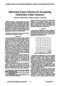
Functions: Genetic operators are designed to build optimal feature sets by evolving and interchanging sub-optimal sets. We defined the evolutionary process using the following functions, tournament selection, uniform crossover, and standard mutation. Tournament selection operates by randomly selecting a set number of candidates, from which the two fittest chomosomes survive. The survivors, called the parent chromosomes, are then subjected to crossover and mutation. Uniform crossover uses a randomly generated binary bit mask to determine which genes (features) are to be crossed. Mutation occurs, with a very low probability, on one or more of any of the alleles within a candidate. If the feature is chosen to mutate it has equal probability of becoming any of the remaining features. The resulting two chromosomes are passed to the next generation for evaluation, and the cycle is repeated until the population is replenished. Figure 2 illustrates the evolution of two child chromosomes.
1.Population
Random selection with replacement
16 45
7 1
37 57
2.Evaluate Fitness .21
69
Random selection without replacement
3.Tourname nt Selection Rank
.46
24
Feature Box 26
4
17
3
.13
80
22
16
69
.54
2
45
37
15
.08
tournament size =3
1
80
22
2
45
1
3
2
45
16 57
69 24
37
15
Select top 2
4.Uniform Crossover Probability = 0.9 Mask
0
1
0
0
Parent 1
80
22
16
69
45
1
57
24
Child 1
80
1
Child 2
45
22
5.Mutation Probability = 0.1
Send Child Chromosomes to the next Generation
.35
.67
.02
.89
.22
.98
.45
.15
80
1
16
69
45
22
57
24
80
1
50
69
45
22
57
24
Parent 2
16
57
69
24
Figure 3 Genetic algorithm sequence using a population of 5, tournament selection, uniform crossover, and standard mutation
Evaluation: To evaluate the feature set candidates we use the predicted accuracy of the classifier. Debate over how to best predict the accuracy of a particular classifier is covered in the statistical literature [16,17]. Cross-validation, bagging, and smoothed leave one out are some of the error estimate methods commonly used. For the purpose of this experiment we chose 10-fold cross-validation (10xCV) applied to the set of true positive detections, which works by holding out a portion of the data for testing, (ten percent, in 10xCV), and training on the remaining data. This process is repeated 10 times, each time leaving out a different portion of the data, such that each case is tested exactly once. The test results provide us with a sensitivity measure. To calculate specificity, we withheld a randomly selected subset of 100 false positive detections for training, and tested on the remaining 700 false detections. We calculate sensitivity, specificity and combine both measurements to get an overall estimate of fitness.
2.2 Forward Stepwise Search Algorithm The forward stepwise search (FSS) algorithm is a classic feature selection technique. The pitfalls of this method include a high susceptibility to getting trapped by local optima, and a one track process that easily discards a feature entirely after a single consideration of its usefulness. However, since variations of 106
Proc. of SPIE Vol. 5031
this method are still widely used in much of the literature on variable reduction [15,18,19], it is important to compare its performance with that of the GA. One method of FSS begins by selecting the single best performing feature as a seed. It then steps through each subsequent feature, adding it to the set if it improves the accuracy measurement, and discarding it otherwise. Each feature has only one chance to survive, which limits the possible combinations. For the purpose of our experiment, the algorithm was slightly modified. Once the feature set size reaches four features, additional features are evaluated by substituting them in for each feature in the set, one at a time. If the new variable improves the predicted accuracy the old variable is discarded.
3. SETUP AND RESULTS
Frequency
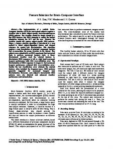
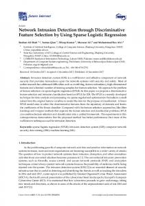
The dataset used contains 207 case studies, with a total of 91 large polyps ( >=1cm), and 33 medium polyps (.5-.9cm). CT colonography was performed using a single detector helical CT scanner. Each patient was scanned in the supine and the prone position. Using the colonoscopy report as the ground truth, a trained observer, under the supervision of a radiologist, manually identified the polyps on the CT scans. A preliminary filter generated a total of 129 true positive detections polyp (multiple detections may correspond to the same polyp) and 2,684 false polyp detections. There are 80 features calculated for each detection. Examples of these features include area, curvature, region density, standard deviation of region density, and wall thickness. A few basic results are observed here. The comparison of the GA with FSS demonstrates the stability of GA. We observe that genetic algorithms are a more consistent method for selecting optimal feature subsets. This is shown by the results of running each algorithm twenty times and observing the differences in the best feature set selected each time. In figure 4 we can clearly see that there are a handful of features that GA repeatedly identifies, whereas FSS is relatively inconsistent. It is not required that GA will always find the same feature set, but we can better interpret the variable’s importance from its consistent selection within the GA scheme. On the other hand, it is hard to draw any conclusions concerning variable importance by plotting the performance of FSS. GA
20 18 16 14 12 10 8 6 4 2 0 1
4
7
10 13 16 19 22 25 28 31 34 37 40 43 46 49 52 55 58 61 64 67 70 73 76 79
Frequency
Feature
FSS
20 18 16 14 12 10 8 6 4 2 0 2
5
8 11 14 17 20 23 26 29 32 35 38 41 44 47 50 53 56 59 62 65 68 71 74 77 80 Feature
Figure 4 Frequency of feature selection over 20 runs for the GA (top) and FSS (bottom).
Proc. of SPIE Vol. 5031
107
Table 2 gives the average sensitivity, specificity, and overall accuracy of the base classifiers selected over all 20 runs, along with standard errors. This comparison demonstrates a statistically significant benefit of GA over FSS. On average, GA was able to significantly increase the specificity of the classifier without reducing the optimal sensitivity found.
Sensitivity ± std error Specificity ± std error 80.6% ± 0.8% 69.4% ± 0.7% 78% ± 2.2% 51.1% ± 3.6% Table 2 (average over 20 runs)
Genetic Algorithm Forward Stepwise
Combined ± std error 75% ± 0.4% 65% ± 1.1%
Figure 5 shows the evolutionary plots of a single run of the GA and FSS. Plotted for the GA is the overall predicted accuracy of the best feature set for each generation. Plotted for FSS is the overall predicted accuracy at each step. The initial improvement made by the GA is noticeable, and a consistent upward trend is observed. On the other hand, the fitness value of the FSS algorithm has no distinguishable point of improvement. Furthermore, in this instance of FSS we can see a point at which the fitness decreases for some time. This is an indication that FSS is easily susceptible to the variability that occurs in error estimation (for further information see [16]).
GA 0.9 Fitness
0.8 0.7 0.6 0.5 1
2
3
4
5
6
7
8
9
10
11
12
13
14
15
16
17
18
19
20
Generation
FSS 0.9 0.8 Fitness0.7 0.6 0.5 0
10
20
30
40
50
60
70
80
Step
Figure 5 Shows the evolution of the best overall accuracy values for GA and below shows the evolution of the fitness values for forward stepwise search.
108
Proc. of SPIE Vol. 5031
4. Discussion and Conclusion We have developed a genetic algorithm for variable selection to be used in the case of colonic polyp detection. This method combines stochastic and heuristic techniques to evolve to an optimal feature subset, and we compared its results to a standard forward stepwise search algorithm. The results of our experiments support the use of genetic algorithms over forward stepwise search for feature selection in computer-aided polyp detection. Our work suggests that genetic algorithms are better for interpreting the feature space since they consistently find groups of variables that yield better results. We also find that, on average, the GA is able to increase the specificity of the classifier while maintaining the sensitivity, which plays a significant role in the advancement of CT colonography. Colonic polyp detection using computer-aided diagnosis will be greatly improved by the discovery of well-defined features and optimal feature sets. The process of feature extraction is ongoing. As new features are introduced, a reliable feature selection algorithm is needed to provide an efficient method for deciphering the interactive, highly correlated nature of the many features.
REFERENCES
1. R.M. Summers, A. Jerebko, M. Franaszek, J. Malley, and C.D. Johnson, Colonic Polyps: Complementary Role of Computer-aided Detection in CT Colonography. Radiology, 2002. 225:391399. 2. T. Hastie, R. Tibshirani, and J. Friedman, The Elements of Statistical Learning: Data Mining, Inference and Prediction. New York; Springer; 2001. 3. N. Cristianini, and J. Shawe-Taylor, Support Vector Machines, and other KernelBased Learning Methods. Cambridge University Press; 2000. 4. B. Schölkopf, C. Burges, AJ Smola (eds), Advances in Kernel Methods; Support Vector Learning. MIT Press; 1999. 5.
R. Kohavi, and G. John, Wrappers for Feature Subset Selection. Artificial Intelligence, 1997. 97:273324.
6.
M. Raymer, W. Punch, E. Goodman, L. Kuhn. and A. Jain, Dimensionality Reduction Using Genetic Algorithms. IEEE Transactions on Evolutionary Computation (2000).
7.
E. Cantu-Paz, Feature Subset Selection by Estimation of Distribution Algorithms.
8.
H. Handels, Th.Rob, J.Kreusch, H.Wolff, and S. Popple, Feature Selection for Optimized Skin Tumor Recognition using Genetic Algorithms. Artificial Intelligence in Medicine, 1999. 16:283-297.
9.
F. Brill, D. Brown, and W. Martin, Fast Genetic Selection of Features for Neural Network Classifiers. IEEE Transactions on Neural Networks, 1992. 3(2):324-328.
10. H. Vafaie, Kenneth D.J., Feature Space Transformation Using Genetic Algorithms. IEEE Transactions on Intelligent Systems, 1998. 13(2):57-65. 11. C. Pena_Reyes, and M. Sippe, Evolutionary Computation in Medicine: an Overview. Artificial Intelligence in Medicine, 2000. 19:1-23. 12. S. Ho, C. Liu, and S. Liu, Design of an Optimal Nearest Neighbor Classifier using an Intelligent Genetic Algorithm. Pattern Recognition Letter, 2002. 23(13): 1495-1503. Proc. of SPIE Vol. 5031
109
13. J.R. Koza, M.A. Keane and M. Streeter, Evolving Inventions. Scientific American, February 2003:5259. 14. P. Castillo-Valdivieso, J. Merelo, A. Prieto, I. Rojas, and G. Romero, Statistical Analysis of the Parameters of a Neuro-Genetic Algorithm. IEEE Transactions on Neural Networks, 2002. 13(6): 1374-1394. 15. K.Z. Mao, Fast Orthogonal Forward Selection Algorithm for Feature Subset Selection. IEEE Transactions on Neural Networks, 2002. 13(5): 1218-1224. 16. R. Tibshirani, A comparison of some error estimates for neural network models. Technical Report, Stanford University Department of Statistics; 1995. 17. T.G. Dietterich, Approximate statistical tests for comparing supervised classification learning algorithms. Neural Computation, 10 (7), 1895-1924; 1998. 18. J. Jelonek, Jerzy S., Feature Subset Selection for Classification of Histological Images. Artificial Intelligence in Medicine, 1997. 9:22-239. 19. B. Sahiner, H.P. Chan, N. Petrick, R.F. Wagner, and L. Hadjiiski, Feature Selection and Classifier Performance in Computer-Aided Diagnosis: The Effect of Finite Sample Size. Medical Physics, 2000. 27(7): 1509-1522. 20. A.K. Jerebko, JD Malley, M Franaszek, RM Summers, Multi-network classification scheme for detection of colonic polyps in CT colonography data sets. In press: Academic Radiology; 2003.
110
Proc. of SPIE Vol. 5031