Feature Selection using Linear Classifier Weights: Interaction with Classification Models Dunja Mladenić
Janez Brank
Jožef Stefan Institute Ljubljana, Slovenia Tel.: +386 1 477 3900
Jožef Stefan Institute Ljubljana, Slovenia Tel.: +386 1 477 3900
[email protected]
[email protected]
ABSTRACT This paper explores feature scoring and selection based on weights from linear classification models. It investigates how these methods combine with various learning models. Our comparative analysis includes three learning algorithms: Naïve Bayes, Perceptron, and Support Vector Machines (SVM) in combination with three feature weighting methods: Odds Ratio, Information Gain, and weights from linear models, the linear SVM and Perceptron. Experiments show that feature selection using weights from linear SVMs yields better classification performance than other feature weighting methods when combined with the three explored learning algorithms. The results support the conjecture that it is the sophistication of the feature weighting method rather than its apparent compatibility with the learning algorithm that improves classification performance.
Categories and Subject Descriptors H.3.0 [Information Storage and Retrieval]: Indexing.
General Terms Algorithms, Performance, Experimentation.
Keywords Text classification, information retrieval, vector representation, feature selection, feature scoring, linear SVM, SVM normal.
1. INTRODUCTION In text classification, feature selection is typically used to achieve two objectives: reduce the size of the feature set in the data representation in order to optimize the use of computing resources and to remove noise from the data in order to optimize the classification performance. A number of standard methods, such as stop word removal or linguistic normalization using stemming, are routinely applied and contribute to the reduction of the feature space, memory
Permission to make digital or hard copies of all or part of this work for personal or classroom use is granted without fee provided that copies are not made or distributed for profit or commercial advantage and that copies bear this notice and the full citation on the first page. To copy otherwise, or republish, to post on servers or to redistribute to lists, requires prior specific permission and/or a fee. SIGIR’04, July 25–29, 2004, Sheffield, South Yorkshire, UK. Copyright 2004 ACM 1-58113-881-4/04/0007...$5.00.
Marko Grobelnik
Natasa Milic-Frayling
Jožef Stefan Institute Ljubljana, Slovenia Tel.: +386 1 477 3900
Microsoft Research Ltd Cambridge, United Kingdom Tel.: +44 1223 479 770
[email protected] [email protected]
consumption, and processing time. In addition, features are often scored and ranked using some feature weighting scheme that reflects the importance of the feature for a given task. Only a selected subset of top scoring features is used for further processing. A fundamental question that arises in this practice is the relationship between the scoring method for feature selection and the classification model that further uses these features. Are there compatibility criteria that the two should satisfy in order to yield optimal classification performance? In a study of Naïve Bayes text classifier [6], feature selection based on Odds Ratio scores consistently lead to statistically significant improvements in classification performance in comparison to the full feature set. This was attributed to the fact that the feature selection method was ‘compatible’ with the used classification algorithm. Indeed, based on statistics used in Naïve Bayes and Odds Ratio, one could characterize them as compatible in the sense that the features with higher Odds Ratio weights are expected to be more influential within the Naïve Bayes classifier. Thus, feature selection based on Odds Ratio weights is expected to be effective in tuning the performance of the Naïve Bayes. In order to gain more insight into this question, we use a novel approach of scoring and selecting features based on weights from linear classifiers. More precisely, we consider an iterative procedure that typically involves a subset of training data to train linear Support Vector Machines (SVM) or Perceptron. The weights of the generated model (i.e., the normal to the hyperplane that separates the classes) are applied to rank the features and select a smaller subset. In the second iteration the full set of data is used within the reduced feature space to train the classifiers and then perform classification of new data. We observe how this type of feature selection method combines with its ‘own’ classification model and with others. The second practical issue is how to select features to take into account available computing resources. Is there an effective way to perform feature selection so to optimize performance for the given computing resources? This can, in fact be achieved by using vector sparsity (or density) as the feature selection criteria as suggested in [1]. We explore the performance optimization for several classifiers in conjunction with different feature weighting algorithms. The main contributions of our work include: (1) widening the perspective on the feature selection task by showing how linear classifiers themselves can be used to address that issue, (2) demonstrating how sparsity based feature selection can guide
optimization of computer resource use, and (3) providing empirical data about the behavior of various combinations of feature selection and learning methods which enable us to make an informed conjecture on the compatibility issue for feature selection methods and the learning algorithm. Our experiment results suggest that it is the sophistication of the feature selection method rather than similarity with the underlying learning algorithm (i.e., apparent compatibility with the classification model) that plays the crucial role in optimizing classification performance. In particular, methods such as feature selection using weights of a linear SVM model, which take into account statistical properties of all the features and documents simultaneously, generally tend to perform better than other explored methods across all text learning algorithms examined. The paper is structured in the following way. We first give a brief description of feature selection and text classification methods used in the experiments. Then we describe the experimental set-up and the sparsity based feature selection. We show how sparsity is used to optimize the use of computing resources. We conclude with a summary of observations and an outline of future work.
2. LEARNING ALGORITHMS AND FEATURE SELECTION METHODS In this study we investigate three learning algorithms, Naïve Bayes, Perceptron, and Support Vector Machines (SVM), and three feature weighting methods, Odds Ratio, Information Gain, and weights from linear classification models. We expected that combinations of these methods would provide valuable insight in the nature of feature selection methods and their compatibility with classification models.
2.1 Learning Algorithms Naïve Bayes. We use the multinomial model as described in [5]. The predicted class for document d is the one that maximizes the posterior probability P(c|d) ∝ P(c) Πt P(t|c) tf(t,d), where P(c) is the prior probability that a document belongs to class c, P(t|c) is the probability that a word w, chosen randomly in a document from class c, equals t, and tf(t,d) is the “term frequency”, or the number of occurrences of word t in a document d. Training simply consists of estimating the probabilities P(t|c) and P(c) from the training documents.
Perceptron [8]. This algorithm trains a linear classifier in an incremental way as a neural unit using an additive update rule. Class prediction for a document represented by the vector x is sgn(wTx) where w is a vector of weights obtained during training. Computation starts with w = 0 and considers each training example xi in turn. If the present w classifies xi correctly it is left unchanged, otherwise it is updated according to the additive rule: w ← w + yi xi where yi is the correct class label of the document xi (yi = +1 for a positive document, yi = –1 for a negative one).
Support Vector Machine (SVM) [2]. This algorithm trains a
linear classifier of the form sgn(wTx + b). Learning is posed as an optimization problem with the goal of maximizing the margin, i.e., the distance between the separating hyperplane wTx + b = 0 and the nearest training vectors. An extension of this formulation, known as the soft margin, also allows for a wider margin at the cost of misclassifying some of the training examples. The dual
form of this optimization task is a quadratic programming problem and can be solved numerically. We used the SvmLight v.3.5 program [3] to train the SVM models. This program is particularly suitable for our purposes because of its optimizations for working with linear kernels. We work with linear SVM and Perceptron models because the existing literature on text categorization indicates that, for this problem, the nonlinear versions of these algorithms gain very little in terms of performance.
2.2 Feature Selection Methods All feature selection methods considered here involve assigning a weight to each feature, ranking the features based on the weights, and retaining only a specified number of features.
Odds Ratio. Let P(t|c) be the probability of a randomly chosen word being t, given that the document it was chosen from belongs to a class c. Then odds(t|c) is defined as P(t|c)/[1–P(t|c)] and the Odds Ratio equals to OR(t) = ln[odds(t|c+)/odds(t|c–)]. Obviously, this scoring measure favors features that are representative of positive examples. As a result a feature that occurs very few times in positive documents but never in negative documents will get a relatively high score. Thus, many features that are rare among the positive documents will be ranked at the top of the feature list. Odds Ratio is known to work well with the Naïve Bayes learning algorithm [6].
Information Gain. Here both class membership and the presence/absence of a particular term are seen as random variables, and one computes how much information about the class membership is gained by knowing the presence/absence statistics (as is used in decision tree induction, e.g., in [7]). Indeed, if the class membership is interpreted as a random variable C with two values, positive and negative, and a word is likewise seen as a random variable T with two values, present and absent, then using the information-theoretic definition of mutual information we may define Information Gain as: IG(t) = H(C) – H(C|T) = Στ,c P(C=c,T=τ) ln[P(C=c,T=τ)/P(C=c)P(T=τ)]. Here, τ ranges over {present, absent} and c ranges over {c+, c–}. As pointed out above, this is the amount of information about C (the class label) gained by knowing T (the presence or absence of a given word).
Feature selection based on linear classifiers. Using weights from the SVM classification model for feature selection was suggested in [9] and studied in detail for linear SVM in [1]. Here we extend this idea to general linear classifiers and discuss the procedure by referring to linear SVM and Perceptron. Both SVM and Perceptron, as linear classifiers, output predictions of the form: prediction(x) = sgn(wTx + b) = sgn(Σj wjxj + b). Thus, a feature j with the weight wj close to 0 has a smaller effect on the prediction than features with large absolute values of wj. The weight vector w can also be seen as the normal to the hyperplane determined by the classifier to separate positive from negative instances. Thus we often refer to the procedure as normal based feature selection. One speculates that since features with small |wj|
are not important for categorization they may also not be important for learning and, therefore, are good candidates for removal.
matches the distribution of categories across documents in the full Reuters collection.
A theoretical justification for retaining the highest weighted features in the normal has been independently derived in a somewhat different context in [10]. The idea is to consider the feature important if it significantly influences the width of the margin of the resulting hyper-plane; this margin is inversely proportional to ||w||, the length of w. Since w = ∑i αi xi for a linear SVM model, one can regard ||w||2 as a function of the training vectors x1, ..., xl, where xi = (xi1, ..., xid), and thus evaluate the influence of feature j on ||w||2 by looking at absolute values of partial derivatives of ||w||2 with respect to xij. (Of course this disregards the fact that if the training vectors change, the values of the multipliers αi would also change. Nevertheless, the approach seems appealing.) For the linear kernel, it turns out that
We also use the same 16 categories that were selected in [1] based on a preliminary document classification experiment that involved training the SVM over a smaller training set for the complete set of Reuters categories and classifying a test set of 9,596 documents. The selection criterion was based on two characteristics of a category: the distribution of positive examples in the whole corpus and the precision recall break-even point for the category achieved in the preliminary experiment. These statistics for the selected subset of 16 categories approximately follows the distribution for all 103 categories. The selected set of categories includes: godd, c313, gpol, ghea, c15, e121, gobit, m14, m143, gspo, e132, e13, c183, e21, e142, and c13.
∑i |∂||w||2/∂xij| = k |wj| where the sum is over support vectors and k is a constant independent of j. Thus the features with higher |wj| are more influential in determining the width of the margin. The same reasoning applies when a non-linear kernel is used because ||w||2 can still be expressed using only the training vectors xi and the kernel function. Note that the normal-based approach to feature weighting and selection involves an important issue: the selection of a set of instances over which one trains the normal w in order to arrive at the feature weights. Since training an SVM model requires a considerable amount of CPU time, and practically requires all the training vectors to be present in main memory all the time, it is desirable to use a subset of the training data in order to facilitate features selection and then retrain the classifier1 over the full data set but using the reduced feature space. Furthermore, it is useful to explore how the selection of the training set affects feature selection and the performance of the final classifier. We illustrate these issues by applying normal based feature selection to different samples of the training data: the full set, one quarter and one sixteenth of the full data size.
3. EXPERIMENT DESIGN 3.1 Data Experiments conducted in this study use data from the Reuters Corpus (http://about.reuters.com/researchandstandards/corpus/) Volume 1 and a sample of 16 categories from the set of 103 categories that comprise the Reuters classification scheme. The experimentation setup is similar to the study presented in [1]. The full Reuters corpus of 806,791 news articles (dated from 20 August 1996 through 19 August 1997) is divided into a “training period” that includes 504,468 articles and a “test period” with the remaining 302,323 documents. For training we used a sample of 118,294 documents from the training period and tested the classifiers on the complete document set from the test period. As described in [1], the selected subset of training data closely
1
Training over the full data set and using the resulting normal to select the features for the second re-training phase makes sense only if the two-phase approach considerably improves the performance and thus justifies the processing cost.
A document may belong to one or more categories; therefore, we regard each category as a standalone binary classification problem where the task is to predict if a document belongs to this category or not. Our document representation is based on the bag-of-words model. We convert text of each document into lowercase, remove stopwords (using a standard set of 523 stop-words), and eliminate words occurring in less than 4 training documents. We represent each document as a TF-IDF vector normalized to the unit length, except for Naïve Bayes when we simply use TF term weighting.
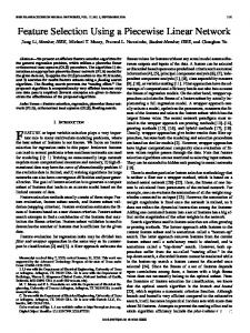
3.2 Sparsity of data representation In order to compare classification performance of several feature selection methods and address the issue of computing resource consumption, we observe the density or, more commonly used term, the sparsity of vectors associated with individual documents. To be precise, we use the term “sparsity” to refer to the average number of terms per document or, more technically, the average number of nonzero components in the vectors by which documents are represented. It has been shown in [1] that the vector sparsity varies significantly when the same number of features is retained for different feature weighting methods. Similarly, a fixed sparsity level yields features sets of very different sizes. This is a rather important observation since it is expected that the performance of the data processing algorithm will depend on the representation of individual documents. As an illustration, Figure 1 shows how specifying the sparsity levels for Odds Ratio, Information Gain, and SVM normal based feature selection affects the performance of the SVM classifier. Each sparsity level is, in turn, achieved by retaining a number of highly scored features. We show the same performance data with respect to the number of features retained for each of the feature selection methods. Sparsity of document vectors, on the other hand, directly affects consumption of computing resources, both the memory for storing the sparse vectors and the time needed to perform calculations. While reducing the total number of features is expected to increase sparsity, the rate at which this is achieved depends on the term weighting scheme, or ultimately the corpus properties such as term distribution (i.e., number of documents in the corpus, or labeled by a particular class, that contain the term). For examples, if the number of features to be retained is fixed, weighting schemes that lead to retaining rare features generally incur a low cost to data storage and calculations. The opposite is true for weighting schemes that favor features common across documents.
M acroaveraged F1, full training set
0.7
0.7
0.65
0.65
0.6
0.6
A verage F1 over the test set
Average F1 over the test set
M acroaveraged F1, full training set
0.55
0.5
0.45
0.55
0.5
0.45
0.4
0.4
0.35
0.35 10
100
1000
10000
100000
Number of features retained after feature selection odds ratio
information gain
svm-1
1
10
100
Average number of nonzero components per vector over the training set odds ratio
perceptron-1
information gain
svm-1
perceptron-1
Figure 1. Macroaverages of F1 measure for the SVM classifier for various feature set sizes and different feature weighting methods. The chart on the left shows the performance against the number of features while the one on the right shows performance at various sparsity levels. The sparsity-based charts allow for a more useful comparison of feature selection methods; e.g., Odds ratio is quite successful at very sparse representations, even though it uses a large vocabulary. Thus, just specifying a fixed number of features does not allow for a reliable control over resource consumption. For that reason, we propose to work directly with the requirement on the sparsity level as the cut-off criterion for feature selection.
3.3 Evaluation measures In our analyses we use standard evaluation measures: precision p and recall r of the classifier, the combined measure F1 defined as F1 = 2pr/(p+r), and precision-recall break-even (BEP) point. Because of the space limitation we report only statistics for the F1 measure, in particular the macroaverages of F1 (calculated for each experiment as the average F1 measure over all categories). Analyses based on microaveraged statistics provide qualitatively similar results.
4. RESULTS 4.1 Effects of feature selection on classification performance In addition to two standard feature weighting methods, Odds Ratio and Information Gain, we report classification results for data representations obtained by normal based feature selection using linear SVM and Perceptron. For both SVM and Perceptron linear classifier we use three sets of training data to obtain feature sets and corresponding weights: the full training set and randomly chosen subsets of 1/4 and 1/16 of the documents. Training the classifiers on these sets results in three normal vectors for each method: svm-1, svm-1/4, and svm-1/16 for the linear SVM and perceptron-1, perceptron-1/4, perceptron-1/16 for the Perceptron. These 6 feature rankings are considered, together with the Odds Ratio and Information Gain, for feature selection and training of the classifiers. For each rank in the list of features we can calculate the average sparsity of vectors achieved if only features from that rank and
above were retained. Similarly, given a sparsity requirement we can find the cut off rank below which the features are discarded in order to achieve the specified vector sparsity. It is interesting to note that specifying sparsity leads to nonuniform number of features across categories, depending on the distribution characteristics of features typical for the category. This is in contrast with the common practice of specifying the fixed number or percentage of top ranking features to be used for all categories. For each of the nine sets of features we train the learning algorithms: Naïve Bayes, Perceptron, and linear SVM, over the training data represented by the reduced set of features. We specify the reduction level in terms of the desired sparsity of vectors. In particular, both Perceptron and SVMs, are in this phase retrained over the full training set, represented by the reduced set of features. The resulting classifiers are then applied to the test data. The charts in Figure 2 show the macroaveraged F1 performance statistics for specific levels of vector sparsity on the horizontal axes: 2, 2.5, 5, 10, 20, 40, and 80 terms per document, as well as for the sparsity of the full document vectors, about 88.3 terms per document on average.
Naïve Bayes Our experiments with Naïve Bayes confirm the known fact that Naïve Bayes benefits from appropriate feature selection [6]. Detailed analysis shows that this is particularly true for categories with smaller number of training data, while for the largest few categories there is little or no improvement from feature selection. Odds Ratio seems to work well with Naïve Bayes when documents are made moderately sparse, 10 to 20 terms per document (which, on average, requires 4000 to 8000 of the best features to be retained) but not extremely sparse. On the other hand, earlier research found that Odds Ratio works well even if
only a few hundred features were kept [6]. Thus, it would be worth exploring whether sparsity is a more reliable parameter in predicting classifier performance than the number of features retained.
Naive Bayes, M acroaverages
Average F1 over the test set
0.54
Information Gain, on the other hand, works well when documents retain about 2.5 terms on average per document, which corresponds to keeping around 70 best features on average (the actual number varies considerably from one category to another, with e13 needing as few as 29 and ghea as many as 163).
0.49
0.44
0.39
0.34 1
10
100
Average number of nonzero components per vector over the training set odds ratio svm-1
information gain perceptron-1/16
svm-1/16 perceptron-1/4
svm-1/4 perceptron-1
Still higher performance with Naïve Bayes can be achieved with feature selection based on Perceptron and linear SVM weights. For SVM, this is true even if much smaller data sets are used in the feature selection phase. Table 1 provides detailed performance results. However, as it can be seen from Figure 2, even with the best of the tried feature selection methods, Naïve Bayes cannot match the performance of the Perceptron and the linear SVM classifiers.
Perceptron, M acroaverages
Table 1. This table shows, for each feature selection method, the best Naïve Bayes classification performance and the sparsity at which it was achieved.
Average F1 over the test set
0.55
0.45
Sparsity which yielded best performance
Macroaveraged F1 at that sparsity
Odds Ratio
20
0.4683
Information Gain
2.5
0.4648
5
0.5208
svm- /4
5
0.5356
svm-1
5
0.5421
10
0.4715
perceptron- /4
10
0.4887
perceptron-1
10
0.5005
Feature selection/ranking method
0.35
0.25
0.15
svm-1/16 1
0.05 1
10
100
Average number of nonzero components per vector over the training set odds ratio svm-1
information gain perceptron-1/16
svm-1/16 perceptron-1/4
svm-1/4 perceptron-1
perceptron-1/16
Linear SVM , M acroaverages
1
0.7
Average F1 over the test set
0.65
Perceptron
0.6
0.55
0.5
0.45
0.4
0.35 1
10
100
Average number of nonzero components per vector over the training set odds ratio svm-1
information gain perceptron-1/16
svm-1/16 perceptron-1/4
svm-1/4 perceptron-1
Figure 2. Macroaveraged F1 performance of different feature selection methods in combination with different machine learning algorithms. Note different scales for F1 values on the vertical axes. The horizontal axes refer to sparsity, the average number of nonzero components per training vector. In this case, this is the average number of terms per training document after terms rejected by feature selection have been removed).
Our experiments show that the Perceptron learning algorithm does not combine well with the feature selection methods considered here. The only case in which performance is actually improved is for the sparsity level of 80 terms per document with perceptron-1, thus a slight reduction in sparsity from 88.3 when all features are used. It is worth noting that the reduction of 8 features on average per document corresponds to retaining around 32,500 out of 75,839 original features. The associated increase in F1, although statistically significant, is marginal (0.8 %). Otherwise, performance drops quickly and considerably as more and more features are discarded. When using SVM-based rankings, the performance is lower although the differences with respect to the Perceptron weighting are small. They are greatest when both feature selectors are allowed to inspect the full document set: perceptron-1 may achieve F1 values up to 2.5 % above those achieved by svm-1 at the same sparsity. The differences between perceptron-1/4 and svm-1/4 and between perceptron-1/16 and svm-1/16 are smaller and often insignificant. Thus, in scenarios when it is desirable to reduce the feature set by first training linear models over smaller
training data sets the two feature scoring methods combine equally well with the Perceptron as the classifier. Furthermore, while the SVM-based feature rankings achieve lower precision and lower F1 values than the Perceptron ones, they tend to have higher recall and break-even point for the same subset of training documents. In combination with the Perceptron classifier, feature ranking by the Information Gain criterion usually performs worse than the rankings of linear classifiers. The difference is slight but statistically significant. On the other hand, the feature ranking by Odds Ratio performs much worse (interestingly, it combines well with the SVM; see the next section). We speculate that the Perceptron type training, which considers individual documents sequentially, is negatively affected by the tendency of Odds Ratio to favor features characteristic of positive documents, in particular those that are rare and absent from negative documents. It would be interesting to see whether Perceptron models with margins [4] are more robust in that respect.
Linear SVM Similarly to Perceptron, the linear SVM does not benefit from feature selection but is much less sensitive to the reduction of the feature space. Here one can reduce the feature set to 10 terms per document on average, while still losing only a few percent in terms of the F1 performance measure. As in the case of Perceptron, statistically significant (though rather small) improvements to the F1 performance in comparison to the full feature set are achieved only when using svm-1 or perceptron-1 feature sets, thus increasing the sparsity from 88.3 to 80 terms per document on average. Odds Ratio works well in combination with the linear SVM classifier, particularly when very sparse documents representations are required. Indeed, at sparsity ≤ 20 it is significantly better than Information Gain. There it also outperforms svm-1/16. At more extreme levels of sparsity it performs better than svm-1/4 and even svm-1 (for sparsity ≤ 2.5). An interesting observation is that the Perceptron-based feature weightings perform much worse with the SVM classifier than the SVM-based weightings. Both feature weighting methods performed quite similarly in combination with the Perceptron as the classifier (see previous section). In addition, perceptron-1 is generally not significantly better than perceptron-1/4, and for extremely sparse documents it is, in fact, significantly worse. Looking at precision and recall separately shows that Perceptron-based feature rankings have particularly poor recall. From sparsity curves that show how the density of document vectors increases with the number of features retained we conclude that the Perceptron-based feature weighting has greater preference for rare features than SVM-based (although not nearly so great as Odds Ratio), especially for features typical of positive documents. We speculate that this may be the cause of poor recall (consequently, poor F1). Interestingly, Information Gain tends to produce high precision but relatively low recall, whereas the opposite holds for Odds Ratio. The SVM-based rankings, on the other hand, are good at both precision and recall, particularly the latter.
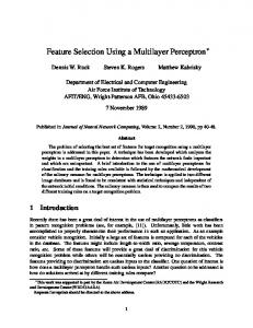
4.2 Feature selection in the memory constraint scenario When text classification is performed with limited memory resources we have a choice of limiting the number of documents used for training or limiting the feature set used to represent the documents or both. The question is how this trade-off affects the performance of the system. (For some training algorithms, such as Naïve Bayes or Perceptron, this is not really a problem, because only (one or more) sequential passes through the training data are needed for training. SVM, on the other hand, requires more or less random access to training documents, which must therefore be kept in main memory during training [11].) Suppose that we have N training documents, and their vectors have S nonzero components on average; thus, M = N⋅S units of memory are required to store the training set. If only M/4 units of memory are available, one could use full vectors of just N/4 training documents; or use feature selection to reduce vectors to sparsity S/2 and work with N/2 training documents, etc. In general, if one needs to reduce memory consumption to M/A, one could keep N/a training documents and use sparsity of S/(A/a) terms per document where a ∈ [1, A]. Thus for a given A we are seeking a for which classification performance is the best. Figure 3 shows the performance of different learning algorithms for A = 1, 2, 4, 8, 16 and a = 1, 2, 4, …, A with SVM weights used in feature selection. Each line corresponds to a fixed memory level requirement: M, M/2, M/4, M/8, and M/16 and the plotted points to F1 measures corresponding trade-off values (e.g., for M/4 these values are: (N/4, S), (N/2, S/2), (N, S/4)). For the Naïve Bayes learner, we observe the expected result: feature selection improves performance and, therefore, for all values of memory reduction A, maximally reducing the feature set to sparsity S/A is best. Of course, the performance increases with the number of training examples used. However, most of the improvement comes from feature selection rather than the increase of the training set. Perceptron, on the other hand, suffers from feature selection so much that keeping fewer documents and using the complete feature set works best, i.e., a = A is the best choice; even doubling the number of documents cannot offset the loss of performance caused by the removal of features. The most interesting behavior is observed with the SVM classifier. Here, non-trivial trade-offs provide best results. For example, for the memory constraint M/2, the trade-off point (N/2, S) yields F1 = 67.3 while (N, S/2) results in an increase to F1 = 68.4. Similarly, for the memory constraint of M/4 we have the following trade-offs: (N/4, S) Æ F1 = 65.2, (N/2, S/2) Æ F1 = 66.5 and (N, S/4) Æ F1 = 67.0. Thus, for the SVM classifier it is generally better to increase the sparsity in order to include a larger number of training examples.
5. CONCLUSIONS Our experiments show that feature scoring and selection based on the normal obtained from the linear SVM combines very well with all the classifiers considered in the study. In particular, in combination with the Naïve Bayes classifier it seems to be far more effective than Odds Ratio for all levels of sparsity below 40 features per vector. Even the Perceptron produces much better feature rankings for Naïve Bayes than Odds Ratio. On the basis of
this observation our conjecture is that, on our dataset, the complexity and sophistication of the feature scoring algorithm plays a larger role in the success of the feature selection method than its compatibility in design with the classifier. Indeed, at the first glance it seems that the Odds Ratio, which closely follows the feature scoring used within Naïve Bayes, should provide the best selection for that classifier. However, a method like SVM that tunes the normal by taking into account all the data points simultaneously seems to be most successful in scoring features.
Performance at fixed memory usage and different choices regarding the sparsity vs. training set size tradeoff. Feature selection uses SVM normal, training with naïve Bayes.
M acroaveraged F1
0.55 0.5 0.45 0.4 0.35 0
10
20
30
40
50
60
70
80
90
Average number of nonzero components per training vector M/16
M/8
M/4
M/2
M
Performance at fixed memory usage and different choices regarding the sparsity vs. training set siz e tradeoff. Feature selection uses SVM normal, training with perceptron. 0.6 Macroaveraged F1
0.55 0.5 0.45 0.4 0.35 0.3 0.25 0.2 0
10
20
30
40
50
60
70
80
90
Average number of nonzero components per training vector M/16
M/8
M/4
M/2
M
Performance at fixed memory usage and different choices regarding the sparsity vs. training set size tradeoff. Linear SVM was used both for training and for feature selection.
Macroaveraged F1
0.69 0.67 0.65 0.63 0.61 0.59 0.57 0.55 10
20
30
40
50
60
70
80
90
Average number of nonzero components per training vector M/16
M/8
M/4
M/2
In the experiments with the memory constraint, we have seen that the Perceptron classifier does not allow for a trade-off since it is adversely affected by feature selection while Naïve Bayes always benefits from feature selection. SVM classifier, on the other hand, can benefit from combining feature selection and adjustment of the training set to fit the memory constraint. Namely, although SVM classifier does not improve with feature selection itself (Section 4.1, subsec. Linear SVM), it yields better performance if feature selection allows a larger training set to be used to train the final model after feature selection. Sparsity of vectors representing the data has been found to be useful for comparing different feature selection methods, particularly because the learning algorithms are more sensitive to sparsity rather than to the number of features as such.
0.71
0
SVM feature ranking combines relatively well with the Perceptron classifier considering the rather dramatic negative effect of feature selection on the Perceptron. One could argue that, because the perceptron-1 is the best performing feature ranking with the Perceptron classifier, the conjecture we proposed in section 1 is weakened. However, when we consider smaller subsets of the training data (e.g., N/4) and look for higher performance levels (F1 > 0.45) of the Perceptron classifier we see that SVM-based and Perceptron-based feature selection have almost identical effect. This makes us believe that our conjecture is in the right direction.
M
Figure 3. Comparison of various combinations of feature selection and training set reduction. Each line connects combinations that have equal memory requirements expressed in terms of the memory M required to represent the entire training, without feature selection applied. The performance varies depending on how the training algorithm reacts to the tradeoff between feature selection and sampling of the document set. If we follow a line for a particular memory requirement from left to right, the representation of documents is more and more complete (i.e., fewer features were discarded) and fewer training documents are used to train the classifier after feature selection. Feature selection is here based on the feature set ranked by normals built from the largest training set that fits the memory requirements (e.g., if the memory limit is M/4, then ¼ of all training documents is used to learn the model and apply feature selection).
Finally, as has been found by other researchers in the field of text categorization, our experiments confirm that SVM outperforms Perceptron and Naive Bayes as a learning algorithm for text categorization. Our further work will expand this study to additional classifiers and data sets, including scenarios that do not necessary involve text data.
6. REFERENCES [1] Janez Brank, Marko Grobelnik, Nataša Milić-Frayling, and Dunja Mladenić. Feature selection using support vector machines. Proc. of the 3rd Int. Conf. on Data Mining Methods and Databases for Engineering, Finance, and Other Fields, Bologna, Italy, September 2002. [2] Cortes, C., Vapnik, V.: Support-vector networks. Machine Learning, 20(3):273–297, September 1995. [3] Thorsten Joachims. (1999). Making large-scale support vector machine learning practical. In B. Schölkopf et al. (Eds.), Advances in kernel methods: Support vector learning. MIT Press, 1999, pp. 169–184. [4] Werner Krauth and Marc Mézard. Learning algorithms with optimal stability in neural networks. Jour. Physics A 20, L745–L752, August 1987.
[5] Andrew McCallum and Kamal Nigam. A comparison of event models for Naïve Bayes text categorization. AAAI Workshop on Learning for Text Categorization (pp. 41–48). AAAI Press, 1998. [6] Dunja Mladenić and Marko Grobelnik. Feature selection for unbalanced class distribution and Naïve Bayes. Proc. 16th Int. Conf. on Mach. Learning. San Francisco: Morgan Kaufmann, pp. 258–267, 1999. [7] J. Ross Quinlan. Constructing decision trees. In: C4.5: Programs for machine learning, pp. 17–26. Morgan Kaufmann, 1993. [8] Frank Rosenblatt. The Perceptron: A probabilistic model for information storage and organization in the brain. Psych. Review 65(6), 386-408. Reprinted in: J. A. D. Anderson, E. Rosenfeld (Eds.), Neurocomputing: foundations of research. Cambridge, MA: MIT Press, 1988.
[9] Vikas Sindhwani, Pushpak Bhattacharya, and Subrata Rakshit. Information theoretic feature crediting in multiclass Support Vector Machines. 1st SIAM Int. Conf. on Data Mining (SDM 2001), Chicago, IL, USA, April 5–7, 2001. SIAM, 2001. [10] Lawrence Shih, Yu-Han Chang, Jason Rennie, David Karger. Not too hot, not too cold: The Bundled-SVM is just right! Workshop on Text Learning (TextML-2002), ICML, Sydney, Australia, July 8, 2002. [11] Soumen Chakrabarti, Shourya Roy, Mahesh V. Soundalgekar: Fast and accurate text classification via multiple linear discriminant projections. Proceedings of the 28th International Conference on Very Large Data Bases (VLDB 2002), Hong Kong, China, August 20--23, 2002, pp. 658–669.