Lecture Notes in Computer Science
1
Featureless Pattern Recognition in an Imaginary Hilbert Space and its Application to Protein Fold Classification Vadim Mottl1, Sergey Dvoenko1, Oleg Seredin1, Casimir Kulikowski2, and Ilya Muchnik2 1
2
Tula State University, Lenin Ave. 92, 300600 Tula, Russia
[email protected] Rutgers University, P.O. Box 8018, Piscataway, NJ 08855, USA
[email protected]
Abstract. The featureless pattern recognition methodology based on measuring some numerical characteristics of similarity between pairs of entities is applied to the problem of protein fold classification. In computational biology, a commonly adopted way of measuring the likelihood that two proteins have the same evolutionary origin is calculating the so-called alignment score between two amino acid sequences that shows properties of inner product rather than those of a similarity measure. Therefore, in solving the problem of determining the membership of a protein given by its amino acid sequence (primary structure) in one of preset fold classes (spatial structure), we treat the set of all feasible amino acid sequences as a subset of isolated points in an imaginary space in which the linear operations and inner product are defined in an arbitrary unknown manner, but without any conjecture on the dimension, i.e. as a Hilbert space.
1
Introduction
The classical pattern recognition theory deals with objects represented in a finitedimensional space of their features that are assumed to be defined in advance, before real objects subject to classification are observed. The emphasis on the feature-based representation of objects is reflected in the name of the most popular method of machine learning for pattern recognition called the support vector method [ 1,2]. At the same time, there exists a wide class of applications in which it is easy to evaluate some numerical characteristics of pairwise relationship between any two objects, but it is hard to indicate a set of rational individual attributes of objects that could form the axis of a feature space. As an alternative to the feature-based methodology, R. Duin and his colleagues [3,4,5] proposed a featureless approach to pattern recognition, in which objects are assumed to be represented by appropriate measures of their pairwise similarity or dissimilarity. It is just this idea we use here as a basis for creating techniques of protein fold class recognition, i.e. allocating a protein, given by the primary chemical structure of its polymerous molecule as a sequence of amino acids (to be exact, their residues) from the alphabet of 20 amino acids existing in nature, over a finite set of typical spatial structures, each associated with a specific manner in which the primary amino acid chains fold in space under a highly complicated combination of numerous This
work is supported, in part, by the Russian Foundation of Basic Research, Grant No. 99-01-00372, and the State Scientific Program of the Russian Federation “Promising Information Technologies”.
Lecture Notes in Computer Science
2
physical forces [6,7]. We lean here upon the compactness hypothesis that is understood as the tendency of proteins with “similar” amino acid chains to belong to the same fold class [8]. It is common practice in computational biology to measure the proximity between two amino acid chains as the logarithmic likelihood ratio of two hypotheses, the main hypothesis that both of them originate from the same unknown protein as result of independent successions of local evolutionary mutations versus the null hypothesis that the chains are completely occasional combinations over the alphabet of 20 amino acids [9]. The generally accepted way of measuring such a likelihood ratio is calculating the so-called alignment score between two amino acid sequences, which is based on finding an appropriate consensus sequence from which both sequences might be obtained as result of as a small number of local corrections as possible, namely, deletions, insertions and substitutions of single amino acids [10,11]. By its nature, the logarithmic likelihood ratio may take as positive as well negative values. In addition, such a ratio calculated for an amino acid sequence with itself gives different values for different proteins. As a result, it is hard to interpret the pairwise alignment score as a similarity measure. In this work, we pose the heuristic hypothesis that the set of all feasible amino acid sequences may be considered as a subset of isolated points in an imaginary Hilbert space in which the linear operations are defined in an arbitrary unknown manner, and the role of inner product is played by the alignment score between the respective pair of amino acid chains. Such an assumption allows for treating the sought-for decision rule of pattern recognition by the principle “one class against another one” as a discriminant hyperplane immediately in the Hilbert space of objects. However, the absence of coordinate axes prevents from finding the “direction element” of the hyperplane, i.e. an element of the Hilbert space that splits all the space points into two nonintersecting regions by values of scalar products with it. Therefore, we propose to use an assembly of selected “representative” objects as a basis in the Hilbert space of all the feasible objects. The elements of the basic assembly are not assumed to be classified, their mission is to serve as coordinate axes of a finite-dimensional subspace, onto which any new object, including those forming the classified training sample, could be projected by calculating inner products with the basic elements. The idea of making distinction between the unclassified basic assembly and classified training sample appears to be quite reasonable for the problem of protein fold class recognition, because the number of proteins whose spatial structure is known is much less than the number of proteins with known amino acid chains.
2
The problem of protein fold class recognition
The problem of finding the spatial structure of a protein represented by its primary amino acid sequence is a challenge posed by the nature. On the one hand, the necessity of such algorithms is dictated by the fact that application of usual physical techniques of magnetic resonance and X-ray analysis is problematic in most cases. Although the number of proteins whose spatial structure is known ever grows, the gap between the number of known amino acid sequences and that of known spatial structures is increasing dramatically. On the other hand, the “existence theorem” is proved by nature itself, because it has been never observed that an amino acid chain had more than one spatial structure. Each protein has its specific spatial organization which does not coincide with that of any other protein. The main principle of establishing the spatial structure of a given
Lecture Notes in Computer Science
3
protein from its amino acid chain consists in finding, for the given chain, the most appropriate structure from a bank of known structures and their fragments. For each amino acid residue in the chain forming a protein of a known structure, the vector of some quantitative features is evaluated which are assumed to be responsible for the spatial position of this residue in the three-dimensional structure. The succession of such features along the amino acid chain is called the profile of this structure. The same features are evaluated for the amino acid chain of the new protein, whereupon the succession obtained is compared with profiles of known structures by alignment of positions in this succession and in the respective profile with respect to eventual insertions and deletions. Such a principle named threading [6] is fraught with enumeration of a large number of known structures. Despite the uniqueness of the spatial structure of each protein, it is the usual case that large groups of evolutionary allied proteins have very similar spatial structures. In this sense, there exist ”much less” spatial structures than primary ones. Of course, the classification of spatial structures is a problem which is not simple, but once a version of classification is accepted, the problem of assigning an amino acid chain to a class of spatial structures falls into the competence area of pattern recognition. In an earlier series of experiments [7], an attempt was made to describe the primary amino acid sequence of a protein by vector of its numerical features and consider it as a point in the respective linear vector space. In particular, the primary structure of a protein was represented by frequencies with which amino acids of the polar, neutral and hydrophobic type and their pairs occur in it. The results of those experiments cannot be assessed as quite successful, to all appearance, because of an immensely rich actual diversity of amino acid properties that may play an important part in forming the spatial structure of a protein. Therefore, we turn here to the featureless formulation of the fold class recognition problem. When studying the structure and properties of proteins, one of commonly used instruments is the characteristic of mutual similarity of two amino acid sequences (a1 ,...,a N ) and (b1 ,...,bK ) given by an appropriate pair-wise alignment procedure (Fig. 1). Procedures of such a kind lean upon a preset similarity matrix for all 210 pairs of 20 amino acids. Such matrices are called substitution matrices and characterize each amino acid pair (a, b) by logarithmic ratio of, first, the probability of their independent occurrence in two amino acid chains pab as result of evolutionary substituting the same unknown amino acid c in a common ancestor chain, and, second, the product of general probabilities qa and qb of their occurrence in arbitrary sequences [9]: (1) s(a, b) log ( pab qa qb ) . The log likelihood ratio s(a, b) is positive if the probability that these two amino acids have a common ancestor is greater than the product of their general probabilities, equals zero in the indifferent case, and is negative if the hypothesis of their common origin is less likely than that of the null hypothesis of their independent occasional appearance. There are several versions of substitution matrices [9,12,13], but each of them is result of observations in large sets of proteins aligned in that or other manner by experienced biologists in accordance with their intuition based, in its turn, on that or other model of evolution. The numerical measure of the proximity of two proteins represented by their amino acid chains is determined as the greatest possible sum of s(a ji , bki ) over all related
Lecture Notes in Computer Science
4
pairs of amino acids ( ji , ki ) , i 1,2,3,..., in a pair-wise alignment with respect to some penalties posed on the presence and length of gaps (Fig. 1): (2) (, ) s(a ji , bki ) gap length penalties . i
In our experiments we used this similarity measure of amino acid chains measured by the commonly adopted alignment procedure Fasta 3 [10,11] with substitution matrix Blossum 50 [9]. As the set of experimental data, we took the collection of proteins selected by Dr. Sun-Ho Kim from Lawrence Berkley National Laboratory in the USA. The collection contains 396 protein domains, i.e. relatively isolated fragments of amino acid chains, chosen from the SCOP Database (Structural Classification of Proteins). The protein domains forming the collection belong to 51 fold classes listed in Table 1. The principle of selection was to provide a low similarity of amino acid sequences within each family, with which purpose only those protein domains were chosen whose similarity (2) to other selected domains did not exceed a preset threshold. Such a principle of selection resulted in protein domain families of different size.
3
The pair-wise alignment score of two amino acid chains as their inner product in an imaginary Hilbert space
It appears natural to interpret the log likelihood ratio for two amino acids s(a, b) (1) as experimentally registered outward exhibition of the actual proximity of their hidden properties. Let these properties be expressed by some hidden vectors y a and y b for which the notion of inner product is defined ( y a , y b ) , then the structure of (1) sug-
gests the idea to consider s(a, b) as a rough measure of it: s(a, b) ( y a , y b ) . By analogy to a single summand, the score of the alignment as a whole (2) may also be interpreted as inner product of the respective combined feature vectors of two proteins (, ) (x , x ) in an imaginary linear feature space. The greater the posi tive value of the similarity, the more “synchronous” are some essential properties of amino acids along the polypeptide chain, the zero value says about full lack of agreement what corresponds to the notion of orthogonality, and a negative value should be interpreted as “opposite phases” of amino acid properties along the chains. However, this is not more than a cursory analogy. For an accurate justification of the hypothesis that there exists a Hilbert space in which the set of proteins could be embedded, we should show that the score matrix of any finite assembly of proteins tends to be nonnegative definite or, at least, can be approximated by such a matrix.
Lecture Notes in Computer Science Table 1. Dr. Kim’s collection of proteins. 1 2 3 4 5 6 7 8 9 10 11 12 13 14 15 16 17 18 19 20 21 22 23 24 25 26
Fold class Globin Cytochrome C Four-helical bundle Ferritin 4-gelical cytokines EF Hand Cyclin Cytochrome P450 Immunoglobin beta – sandwich Common fold of difteria toxin / transcription factors / cytochrome Cupredoxins C2 domain Viral coat and capsid proteins Crystallins / protein S / yeast killer toxin Galastose-binding domain ConA lectins / glucanases OB-fold Beta-Trefoil Reductase / isomerase / elongation factor Trypsin serine proteases Acid proteases PH domain Lipocalings Double-stranded beta-helix Barrel-sandwich hybrid TIM-barrel
Size 12 7 8 8 11 13 4 5 31
27 28 29 30 31 32 33 34 35
5
36
9 3 15 5 4 8 17 5 4 6 5 7 6 6 6 28
37 38 39 40 41 42 43 44 45 46 47 48 49 50 51
Fold class Flavodoxin Adenine nucleotide alpha hydroclase Rossmann-fold domains Thiamin-binding P-loop containing NTP hydrolases Thioredoxin fold Restriction endonucleases Ribonuclease H motif Phosphoribosyltransferases (PRTases) S-adenosyl-L-methionine-dependent methyltransferases Alpha / beta-Hydrolases Phosphorylase / hydrolase Periplastic binding protein I Periplastic binding protein II Lysozyme Cysteine proteinases Beta-Grasp Cystatin Ferredoxin Zincin N-terminal nucleophile aminohydrolases ADP-ribosylation C-type lectin Protein kinases (PK), catalytic core Beta-Lactamase / D-ala carboxypeptidase
Size 9 4 14 3 9 9 5 9 3 5 12 5 7 7 4 4 8 7 20 7 4 4 6 4 3
5
Lecture Notes in Computer Science
6
: TNPGNASSTTTTKPTTTS-----RGLKTINETDPCIKNDSCTG
: GS----ATSTPATSTTAGTKLPCVRNKTDSNLQSCNDTIIEKE i 12 34567 Fig. 1. Fragment of an aligned pair of amino acid chains from the protein family Envelope glycoprotein GP120 in the database Pfam.
We checked this hypothesis for an assembly of 396 proteins (Table 1) by way of calculating all the eigenvalues of the score matrix obtained by the pair-wise alignment procedure Fasta 3 [10,11] with the substitution matrix Blossum 50 [9]. All the eigenvalues turned out to be positive (Fig. 2). The conclusion suggests itself that the pair-wise similarity measure determined by the procedure Fasta 3 possesses properties having much in common with those of inner product. This circumstance should be considered as a reason in favor of the theoretical applicability of the principle of featureless pattern recognition in a Hilbert space to the problem of protein fold class recognition.
18000
0 1
100
200
300
396
Fig. 2. Eigenvalues of Dr.Kim’s collection of proteins: max 16621 , min 304 ; all eigenvalues are positive.
4
Hilbert space of classified objects and optimal discriminant hyperplane
Let the set of all feasible objects under consideration is partitioned into two classes 1 { : g () 1} and 1 { : g () 1} by an unknown indicator function g () 1 . The main idea of the featureless approach to pattern recognition consists in treating the set as a Hilbert space in which the linear operations and inner product are defined in an arbitrary manner under the usual constraints: (1) addition is symmetric and associative , ( ) ( ) ; (2) there exists an origin such that for any element ; (3) there exists the inverse elements () for any ; (4) multiplication by a real coefficient c , c R , is associative (c d ) c(d ) and 1 for any ;
Lecture Notes in Computer Science
7
(5) addition and multiplication are distributive c ( ) c c , (c d ) c d ; (6) inner product of elements is symmetric (, ) (, ) R and linear (, ) (, ) (, ) , (, c ) c (, ) ; (7) inner product of an element with itself possesses the properties (, ) 0 , (, ) 0 if and only if and gives the norm || || (, )1 2 0 .
It is not meant that all the elements of the Hilbert space do exist in reality. We ~ consider really existing objects as making a subset of isolated points in , whereas all the remaining elements are nothing else than products of our imagination. It is ~ just the extension of to what allows speaking about “sums” of really existing objects and their “products” with real-valued coefficients. It is assumed that even if an element of the Hilbert space really exists ~ , it cannot be perceived by the observer in any other way than through its ~ inner products (, ) with other really existing elements . If is a fixed element of the Hilbert space, an imaginary one in the general case, the realvalued linear discriminant function d ( | , b) (, ) b , where b R is a constant, may be used as decision rule gˆ () : {1, 1} of judging on the hidden classmembership of an arbitrary object , might it really exist or not: 0 gˆ () 1, (3) d ( | , b) (, ) b 0 gˆ () 1. Here the element plays the role of the direction element of the respective discriminant hyperplane in the Hilbert space (, ) b 0 . However, we have, so far, no constructive instrument of choosing the direction element and, hence, the decision rule of recognition, because, just as any element of , it can be defined only by its inner products with some other fixed elements that exist in reality. Let the observer have chosen an assembly of really existing objects 0 {10 ,...,0n } , called the basic assembly, which is not assumed to be classified, in the general case, and, therefore, it is not yet a training sample. The basic assembly will play the role of a finite basis in the Hilbert space that defines an n dimensional subspace n (4) n (10 ,...,0n ) : i 1 ai 0i .
We restrict our consideration to only those discriminant hyperplanes whose direction elements belong to n (10 ,...,0n ) , i.e. can be expressed as linear combinations n
(a) ai 0i , a R n .
(5)
i 1
The respective parametric family of discriminant hyperplanes
(a), b
i 1 ai ( , ) b 0 and, so, linear decision rules n
0 i
n 0 gˆ () 1, d | (a), b ai (0i , ) b i 1 0 gˆ () 1,
,
(6)
Lecture Notes in Computer Science
8
will be completely defined by inner products of elements of the Hilbert space with elements of the basic assembly (0i , ) , i 1,...,n . We shall consider the totality of these values for an arbitrary element as its real-valued “feature vector” T (7) x() x1 () xn () R n , x i () (0i , ) .
Mark that if (a), 0 then (0i , ) 0 for all 0i 0 . This means that by choosing the direction elements in accordance with (5) we restrict our consideration to only those discriminant hyperplanes which are orthogonal to the subspace spanned over the basic assembly of objects. As a result, all elements of the Hilbert space that
T
have the same inner products with basic elements x (01 , )(0n , ) , or, in other words, the same projection on the basic subspace n (10 ,...,0n ) (4), will be assigned the same class gˆ () 1 by linear decision rules (6). Therefore, we call the features (7) projectional features of Hilbert space elements. We have come to a parametric family of decision rules of pattern recognition in a Hilbert space (6) that lean upon projectional features of objects: 0 gˆ () 1, (8) . d x() | a, b aT x() b 0 gˆ () 1, Thus, the notion of projectional features reduces, at least, superficially, the problem of featureless pattern recognition in a Hilbert space to the classical problem of pattern recognition in a usual linear space of real-valued features. Let the observer be submitted a classified training sample of objects {1 ,...,N } , g1 g (1 ),...,g N g (N ) , that does not coincide, in the general case, with the basic assembly 0 {10 ,...,0n } . The observer has no other way of perceiving them than to calculate their inner products with objects of the basic assembly, what is equivalent to evaluating their projectional features
x( j ) x1 ( j ) xn ( j ) (10 , j )(0n , j ) R n . T
T
Parameters of the discriminant hyperplane a R n and b R (8) should be chosen so that the training objects would be classified correctly with a positive margin 0 : n when g ( j ) 1, (9) d j | (a), b ai (0i , j ) b aT x( j ) b i 1 when g ( j ) 1. If the training sample is linearly separable with respect to the basic assembly, there exists a family of hyperplanes that satisfy these conditions. It is clear that the margin remains positive after multiplying the pair (a) , b R with a positive coefficient c (a) , c b R , c 0 , thus, it is sufficient to consider direction elements
of a preset norm ||(a) || (a), (a) const . One of them, for which max and the conditions (9) are met, will be called the optimal discriminant hyperplane in the Hilbert space. Because the direction element of the discriminant hyperplane is determined here by a finite-dimensional parameter vector, such a problem, if considered in the basic subspace n (10 ,...,0n ) (4), completely coincides with the classical statement of the pattern recognition problem as that of finding the optimal discriminant hyperplane. The same reasoning as in [2] leads to the conclusion that the maximum margin is 12
Lecture Notes in Computer Science
9
provided by choosing the direction element (a) and threshold b R from the condition (10) ||(a) ||2 min , g j (a), j b 1, j 1,...,N . However, such an approach becomes senseless in case the classes are inseparable in the basic subspace, and the constraints (9) and, hence, (10) are incompatible. To design an analogous criterion for such training samples, we, just as V. Vapnik, admit nonnegative defects g j (a), j b 1 j , j 0 , and use a compromise crite-
rion (, ) C j 1 j min with a sufficiently large positive coefficient C meant N
to give preference to the minimization of these defects. So, we come to the following formulation of the generalized problem of finding the optimal discriminant hyperplane in the Hilbert space that covers both the separable and inseparable case: N 2 ||(a) || C j min, j 1 g aT x( ) b 1 , 0, j j j j
5
(11)
j 1,...,N .
Choice of the norm of the direction element
The norm of the direction element of the sought-for hyperplane can be understood, at least, in two ways, namely whether as that of an element of the Hilbert space or as the norm of its parameter vector in the basic subspace a R n . In the former case we have, in accordance with (5), n
n
|| (a) ||2 (a), (a) (0i , 0l )a i al aT Ma , 2
(12)
i 1 l 1
where M (0i , 0l ), i, l 1,...,n is matrix (n n) formed by inner products of basic elements ,..., , whereas in the latter case 0 1
0 n
n
||(a) ||2 ai2 aT a .
(13)
i 1
In the “native” version of norm (12), the training criterion (11) is aimed at finding the shortest direction element , and, so, all orientations of the discriminant hyperplane in the original Hilbert space are equally preferable. On the contrary, if the norm is measured as that of the vector of coefficients representing the direction element in the space of projectional features (13), the criterion (11) seeks the shortest vector a Rn (13), so that equally preferable are all orientations of the hyperplane in R n but not in . It is easy to see that if and are two arbitrary elements of a Hilbert space , then the squared Euclidean distance from to its projection onto the beam formed by element equals (, ) (, ) 2 (, ) . In its turn, it can be shown [8] that
if
aT a min
j 1 j , (a) n
2
under
the constraint
(a), (a) aT Ma const ,
then
max , and, so, (a) tends to be close to the major inertia axis of
the basic assembly.
Lecture Notes in Computer Science
10
Thus, training by criterion (11) with ||(a) ||2 aT a , i.e. without any preferences in the space of projectional features, is equivalent to a pronounced preference in the original Hilbert space in favor of direction elements oriented along the major inertia axis of the basic assembly of object. As a result, the discriminant hyperplane in the Hilbert space tends to be orthogonal to that axis (Fig. 3). This is out of significance if the region of major concentration of objects in the Hilbert space is equally stretched in all directions. But such indifference is rather an exclusion than a rule. It is natural to expect the distribution of objects be differently extended in different directions, what fact will be reflected by the form of the basic assembly and, then, by the training sample. In this case, a reliable decision rule of recognition exists only if objects of two classes are spaced just in one of the directions where the extension is high. Therefore, it appears reasonable to escape discriminant hyperplanes oriented along the basic assembly even if the gap between the points of the first and the second class in the training sample has such an orientation, and prefer transversal hyperplanes (Fig. 3). It is just this preference that is expressed by the training criterion (11) with ||(a) ||2 aT a min in contrast to ||(a) ||2 aT Ma min .
0i 0 elements of the basic assembly Area of admissible direction elements
j elements of the training sample,g j 1
Admissible direction element (a) with the minimum norm of the coefficient vector || a ||
Isosurfaces of constant norm || a || const in the Hilbert space
j elements of the g 1 training sample, j
a T a min a T Ma min T wo versios of the optimaldiscriminant hyperplanein the Hilbert space
Fig. 3. Minimum norm of the direction vector of the discriminant hyperplane in the space of projectional features as criterion of training. In the original Hilbert space, the discriminant hyperplanes are preferred whose direction elements are oriented along the major inertia axis of the basic assembly.
6
Smoothness principle of regularization in the space of projectional features
Actually, training by criterion aT a min is nothing else than a regularization method that makes use of some information on the distribution of objects in the Hilbert space. This information is taken from the basic assembly and, so, should be considered as a priori one relative to the training sample. In case the distribution is almost degenerate in some directions, it is reasonable to prefer discriminant hyperplanes of
Lecture Notes in Computer Science
11
transversal orientation even if the training sample suggests the longitudinal one as it is shown in Fig. 3. In this Section, we consider another source of a priori information that may be drawn from the basic assembly of objects before processing the training sample. The respective regularization method follows from the very nature of projectional features, namely, from the suggestion that the closer are two objects of the basic assembly, the less should be the difference between the coefficients of their participating in the direction element of the discriminant hyperplane (5). In the feature space of an arbitrary nature, there are no a priori preferences in favor of that or other mutual arrangement of classes, and the only source of information on the sought-for direction is the training sample. But in the space of projectional features different directions are not equally probable, and it is just this fact that underlies the regularization principle considered here. The elements of the projectional feature vector of an object are its scalar T products with objects of the basic assembly x() x1 () xn () Rn ,
xk () (, 0k ) , 0k 0 . The basic objects, in their turn, are considered as elements of the same linear Hilbert space and, so can be characterized by their mutual proximity. If two basic objects 0j and 0k are close to each other, the respective projectional features do not carry essentially different information on objects of recognition , and it is reasonable to assume that the coefficients a j and ak in the linear decision rule should also take close values. Therein lies the a priori information on the direction vector of the discriminant hyperplane that is to be taken into account in the process of training. In fact, the coefficients a j are functions of basic points in the Hilbert space a j a(0j ) , and the regularization principle we have accepted consists in the a priori assumption that this function should be smooth enough. It is just this interpretation that impelled us to give such a principle of regularization the name of smoothness principle. It remains only to decide how the pair-wise proximity of basic objects should be quantitatively measured. For instance, inner products jk ( j , k ) might be taken as such a measure. Then, the a priori information on the sought-for direction element can N be easily introduced into the training criterion aT a C j 1 j min in (11) with
||(a) ||2 aT a as an additional quadratic penalty aT (I B)a C j 1 j min N
where n 1n 11 1i i 1 1 n n T 2 a Ba il ( ai al ) , B , n 2 i 1 l 1 n1 n n n i i 1 and parameter 0 presets the intensity of regularization. Because the size of the training sample N is, as a rule, less than the dimensionality n of the space of projectional features, the subsamples of the first and the second class will most likely be linearly separable. On the force of this circumstance, when solving the quadratic programming problem (11) without regularizing penalty, the
Lecture Notes in Computer Science
12
optimal shifts of objects will equal zero j 0 , j 1,...,N . After introducing the regularization penalty, the errorless hyperplane may turn out to be unfavorable from the viewpoint of a priori preferences expressed by matrix B with sufficiently large coefficient . In this case, the optimal hyperplane will sacrifice, if required, the correct classification of some especially nuisance objects of the training sample, what will result in positive values of their shifts j 0 .
7
Experiments on protein fold class recognition “one against one”
Experiments on fold class recognition were conducted with the collection of amino acid sequences of 396 protein domains grouped into 51 fold classes (Table 1). As the initial data set served the matrix 396 396 of pair-wise alignment scores obtained by alignment procedure Fasta 3 and considered as matrix of inner products of respective protein domains ( j , k ) in an imaginary Hilbert space. In the series of experiments described in this Section, we solved the problem of pair-wise fold class recognition by the principle “one against one”. There are m 51 classes in the collection and, so, m(m 1) 2 1275 class pairs, for each of which we found a linear decision rule of recognition. As the basic assembly 0 {01 ,...,0n } , we took amino acid chains of 51 protein domains, n 51 , one from each fold class. As representatives of classes, their “centers” were chosen, i.e. the protein domains that gave the maximum sum of pair-wise scores with other members of the respective class. Thus, each protein domain was represented by a 51-dimensional vector of its projectional features (7). For each of the 1275 class pairs, the training sample consisted of all protein domains making the respective two classes (Table 1). Thus, the size of the training sample varied from N 7 for pairs of small classes, such as (50) Protein kinases, catalic core and (51) Beta-Lactamase, to N 59 in two greatest classes (9) Immunoglobin beta - sandwich and (26) TIM-barrel. We applied the technique of pattern recognition with preferred orientation of the discriminant hyperplane along the major inertia axis of the basic assembly in the Hilbert space. The quadratic programming problem (11) was solved for each of 1275 class pairs in its dual formulation [2]. A way of empirical estimating the quality of the decision rule immediately from the training sample offers the well-known leave-one-out procedure [2]. One of the objects of the full training sample containing N objects is left out at the stage of training, and the decision rule inferred from the remaining N 1 objects is applied to the left-out one. If the result of recognition coincides with the actual class given by the trainer, this fact is registered as success at the stage of examination, otherwise an error is fixed. Then the control object is returned to the training sample, another one is left out, and the experiment is run again. Such a procedure is applied to all the objects of the training sample, and the percentage of errors or correct decisions is calculated, which is considered as an estimate on the quality of the decision rule inferred from the full sample would it be applied to the general population. In each of 1275 experiments, the separability of the respective two fold classes was estimated by such a procedure. Two rates were calculated for each class pair, namely, the percentage of correctly classified protein domains of the first and the second class. As the final estimate of the separability, the worst, i.e. the least, of these two percentages was taken.
Lecture Notes in Computer Science
13
As a result, the separability was found to be not worse than: 100% in 9% of all class pairs (completely separable class pairs), 90% in 14% of all class pairs, 80% in 32% of all class pairs, 70% in 53% of all class pairs. The separability of 26 classes from more than one half of other classes is not worse than 70%. One class, namely, (50) Protein kinases (PK), catalytic core, showed its complete separability from all the classes. On a data set of a lesser size, we checked how the pair-wise separability of fold classes will change if the number of basic proteins, i.e. the dimensionality of the projectional feature space, increases essentially. For this experiment, we took all the proteins of the collection as basic ones, so that the dimensionality of the projectional feature space became n 396. The same truncated data set was used for studying how the separability of classes is affected by normalization of the alignment scores between amino acid chains, what is equivalent to projection of respective points of the imaginary Hilbert space onto the unit sphere. If (, ) is inner product of two original points of the Hilbert space associated with the respective two protein domains and , the inner product of their projections and onto the unit sphere will be ( , ) (, ) (, ) (, ) . We used these values, instead of (, ) , as similarity measure of protein domain pairs for fold class recognition. For this series of experiments, we selected 7 fold classes different by their size and averaged separability from other classes. The chosen classes that contain in sum 85 protein domains are shown in Table 2. The results are presented in Table 3. As we see, the extension of the basic assembly improved the separability of the class pairs that participated in the experiment. As to the normalization of the alignment score, it led to an improvement with the small basic assembly and practically did not change the separability with the enlarged one. Experimental study of effects of regularization was conducted with the same truncated data set (Table 2). We examined how the smoothness principle of regularization, expressed by the modified quadratic programming problem (4.1, improves the separability of fold classes “one against one” within the selected part of the collection. The separability of each of 21 pairs of classes was estimated by the leave-one-out procedure several times with different values of the regularization coefficient . Each time, the separability of a class pair was measured by the worst percentage of correct decisions in the first and the second class, whereupon the averaged separability over all 21 class pairs was calculated for the current value of . Such a series of experiments was carried out twice, with original and normalized alignment scores. The dependence of the separability on the regularization coefficient in both series is shown in Fig. 4. In both series of experiments, a marked improvement of the separability is gained. The quality of training grows as the regularization coefficient increases, however, the improvement in not monotonic. A slight drop in separability with further increase in the coefficient after the maximum is attained arises from a too deep roughness of the decision rule adjustment.
Table 2. Seven fold classes selected for the additional series of experiments. Fold class
Averaged separability Size from other classes
Lecture Notes in Computer Science 1 3 4 5 10 12 26
Globin Four-helical bundle Ferritin 4-gelical cytokines Common fold of difteria toxin / transcription factors / cytochrome C2 domain TIM-barrel
12 8 8 11 5 3 28
14
73.4 % 70.8 % 60.4 % 66.0 % 65.2 % 8.2 % 52.6 %
Table 3. Averaged pair-wise separability of seven fold classes in four additional experiments. Averaged separability Original score matrix Normalized score matrix
Size of the basic assembly n 51 396
(, )
( , )
63.5 % 76.6 %
69.4 % 75.3 %
Separability (%)
Separability (%) 80
70
80
70.6
70
78.7
69.4
63.5 60
Reglarization coefficient
50
60
Reglarization coefficient
50 5
10
Original score matrix
15
5
10
15
Normalized score matrix
Fig. 4. Dependence of the averaged pair-wise separability over 21 fold class pairs on the regularization coefficient.
8
Conclusions
Within the bounds of the featureless approach to pattern recognition, the main idea of this work is treating the pair-wise similarity measure of objects of recognition as inner product in an imaginary Hilbert space, into which really existing objects may be mentally embedded as a subset of isolated points. Two ways of regularization of the training process follow from this idea, which contribute to overcoming the small size of the training sample. In the practical problem of protein fold class recognition, to embed the discrete set of known proteins into a continuous Hilbert space, we propose to consider as inner product the pair-wise alignment score of amino acid chains, which is
Lecture Notes in Computer Science
15
commonly adopted in bioinformatics as their biochemically justified similarity measure.
9
References
1. Cortes, C., Vapnik, V.: Support-vector networks. Machine Learning, Vol. 20, No.3, 1995. 2. Vapnik, V. Statistical Learning Theory. John-Wiley & Sons, Inc. 1998. 3. Duin, R.P.W, De Ridder, D., Tax, D.M.J. Featureless classification. Proceedings of the Workshop on Statistical Pattern Recognition, Prague, June 1997. 4. Duin, R.P.W, De Ridder, D., Tax, D.M.J. Experiments with a featureless approach to pattern recognition. Pattern Recognition Letters, vol. 18, no. 11-13, 1997, pp. 1159-1166. 5. Duin, R.P.W, Pekalska, E., De Ridder, D. Relational discriminant analysis. Pattern Recognition Letters, Vol. 20, 1999, No. 11-13, pp. 1175-1181. 6. Fetrow J.S., Bryant S.H. New programs for protein tertiary structure prediction. Biotechnology, Vol. 11, April 1993, pp. 479-484. 7. Dubchak, I., Muchnik, I., Mayor, C., Dralyuk, I., Kim, S.-H. Recognition of a protein fold in the context of the SCOP classification. Proteins: Structure, Function, and Genetics, 1999, 35, 401-407. 8. Mottl, V., Dvoenko, S., Seredin, O., Kulikowski, C., Muchnik, I. Alignment Scores in a Regularized Support Vector Classification Method for Fold Recognition of Remote Protein Families. DIMACS Technical Report 2001-01, January 2001. Center for Discrete Mathematics and Theoretical Computer Science. Rutgers University, the State University of New Jersey, 33 p. 9. Durbin, R., Eddy, S., Krogh, A., Mitchison, G. Biological Sequence Analysis. Probabilistic Models of Proteins and Nucleic Acids. Cambridge University Press, 1988. 10. Pearson, W. R., Lipman, D. J. Improved tools for biological sequence analysis. PNAS, 1988, 85, 2444- 2448. 11. Pearson, W. R. Rapid and sensitive sequence comparison with FASTP and FASTA. Methods in Enzymology, 1990, 183, 63-98.