148
trends in analytical chemistry, vol. 16, no. 3, 1997
Feed-forward artificial neural networks: applications to spectroscopy Dragan A. Cirovic Bris to/, UK Applications of multi-layer feed-forward artificial neural networks (ANN) to spectroscopy are reviewed. Network architecture and training algorithms are discussed. Backpropagation, the most commonly used training algorithm, is analyzed in greater detail. The following types of applications are considered: data reduction by means of neural networks, pattern recognition, multivariate regression, robust regression, and handling of instrumental drifts.
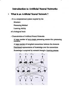
1. Introduction’ Artificial neural networks (ANN) are mathematical models comprised of highly inter-connected processing units, neurones. The theoretical bases of these systems were originally developed within neuroscience. They were subsequently embraced by other branches of science in an attempt to transfer rules governing natural intelligent systems into the sphere of artificial intelligence, in the first instance, and later into many others. The forms of exploitation of natural cognition principles by diverse branches of science often bear very little resemblance to their native counterparts. One of the most important concepts borrowed from the natural cognition research is that of parallel distributed processing (PDP). The PDP is a method of storing and retrieving information from the system which consists of a large number of very simple processing units, with an exceptionally high level of interconnection between the units. Such a system possesses the ability to adjust the strength of connections between its units during the learning stage. The connection strengths (network weights) are means of capturing information. The stored data can be retrieved subsequently by presenting the trained system with the input stimuli. The form of
‘A glossary
appears at the end of this article.
01659936/97/$17.00 PHSO165-9936(97)00007-l
knowledge gathered by neural nets is fundamentally different from that used conventionally by computers, where information is stored in a sequential manner. The PDP systems generalize data, in the sense that they do not allow one-to-one correspondence between physical memory and information units. This, in turn, makes their informationretrieval times much shorter, and their physical storage requirements much smaller, than those offered by sequential systems. The initial experiments with ANNs, which have more than a half-century-long tradition, did not offer much encouragement. This was owing partly to the lack of theoretical foundations, and partly to the inability of the technology of the time to cope with the high computational requirements of ANNs. The more recent advances in information technology coincide with an increase of interest in neural networks, and the last decade can be labelled the most fruitful period in the field. One of the first waves of theoretical advances in the area was reviewed in the book edited by Rumelhart and McClelland [ 11. Since then, ANNs have proved to be useful in a number of fields, including pattern recognition and classification, function approximation, non-linear regression analysis, clustering, combinatorial optimization, robot control, and image compression. The width of scope of applications of ANN comes from their ability to approximate complex functions, which makes them well-suited for modelling non-linear relationships. The developments in recent years have shown increasing growing interest in ANNs among chemists. This process has been catalyzed by a number of excellent tutorials and reviews [ 2-91. The most often used network type was the multi-layer feedforward (MLF) ANN with backpropagation training. It is thought that 90% or more of all applications of ANNs have utilized the feed-forward architecture. The backpropagation training procedure is so common for feed-forward networks that the term ‘backpropagation’ is regularly used to designate both the network architecture and the training procedure. The range of chemical applications of MLF ANN is very large. It includes fields as diverse as: Copyright
0 1997 Elsevier Science B.V. All rights reserved.
trends in analytical chemistry, vol. 16, no. 3, 1997
149
modelling of secondary molecular structure of proteins and DNA, molecular dynamics, quantitative structure-activity relationships (QSAR), quantitative structure-property relationships (QSPR), interpretation of spectra, calibration, and process control. In this article, precedence is given to the spectroscopic applications.
2. Theoretical
foundations
MLF networks belong to a class of supervised learning nets. They require a training data set composed of input/output data pairs. For example, in multivariate calibration one may want to establish a relationship between IR spectra and the corresponding concentration profiles of chemical mixtures. Each sample is characterized by a spectrum (network input) and a concentration profile (the desired output). The inputs are presented to the net, one at a time, usually in random order, and the network outputs are compared to the target outputs in order to adjust network weights. One epoch involves the presentation of all samples to the network. Network training consists of performing a series of epochs until a certain convergence criterion is satisfied. 2.1. Network architecture A MLF ANN consists of an input layer, an output layer, and a variable number of hidden layers. The input layer is not normally counted, because it is only formally present, in the sense that it does not do any processing: for example, a two-layer network consists of the input, hidden, and output layers (Fig. 1). All connections between the layers are allowed. Connections between the nodes of the same layer, as well as the auto-connections (loops), are prohibited. The connections between non-con-
Fig. 2. Fully connected three-layer feed-forward ANN with additional direct connections. The direct connections are symbolically presented as the bold arrows.
secutive layers are called ‘directed connections’. They are symbolically presented with bold arrows, as in Fig. 2. Although the recursive connections are feasible, they require adjustments to be made to the training algorithm. The geometrical disposition of neurones within a layer is an application-specific issue. In spectroscopic applications, layers usually have a linear topology. The optimal network architecture depends on the complexity of the modelled relationship. Generally, error surfaces encountered in quantitative analysis are less complex than those used in qualitative analysis. The methods for determination of the optimal number of hidden layers can be divided into two groups. One of them starts from a very simple network and gradually increases the network complexity until the optimal architecture is found. The methods from the other group attempt to reach the optimum by moving in the opposite direction, i.e. they start from a large network and monitor the effects of reducing the number of hidden layers and connections between the nodes. In either case, a vast amount of redundant computation has to be performed in order to establish the optimum. However, for many practical applications such an extensive search for the optimal network architecture is not justifiable, and an empirical rule which says that the number of adjustable parameters should be approximately a half of the number of samples, can be used instead. 2.2. Network layers
Fig. 1. Fully connected two-layer feed-forward ANN. The threshold nodes are greyed.
In this article, network layers are denoted by the superscripts p = 0, .. . , N (see Fig. 3 and Table 1). The desired output is denoted by the superscript d. The pth layer’s input, GP, and output, yp, are vectors with mp elements each, i.e.
trends in analytical chemistry, vol. 76, no. 3, 1997
150
..I I N
P
U T
m”
Y0
Fig. 3. Schema of an N-layered feed-forward ANN.
I
1. and 2). In the matrix representation of the network (Fig. 3. ) it is assumed that the dimensions of the affected vectors and matrices are accordingly enlarged. 2.3. Training algorithm The most commonly used training algorithm, the backpropagation, is the first-order gradient method. It is known as a steepest decent optimization. Its object or error function, E, is for the sample-wise minimization defined as a sum of squared residuals between the desired and the actual network output
(1)
mN
E(w) = The two successive layers, (p- 1 )th and pth, respectively, are related by means of a weight matrix wp=
(2)
The input to the pth layer is the sum of weighted outputs from the previous layer (JP
=
wPyP-’
(3)
The output of the pth layer lies in a domain of the corresponding transformation function
c
f(OP) = max[O, min(GP,
l)]
function is the (5)
A limitation of this function is that it is not differentiable in its whole domain, which makes it inaccessible to gradient-based training methods. The continuous functions with a similar shape, such as sigmoidal (or logistic) and tanh are used instead (see Fig. 4). These functions are particularly convenient because their derivatives are very simple. The choice between the two functions is basically only dependent on the desired output range. The adaptive ability of the network is greatly enhanced by the use of a constant term referred to as a threshold. This term causes a horizontal shift of the transformation curve, i.e. the threshold of the graphs in Fig. 4 is zero. A common way of implementing thresholds is to add to each network layer an extra node with a constant value of one (see Fig.
(6)
E(W’, .. .. WN)=E(w).
The backpropagation training is a process of step-wise modification of weights in the direction of the maximal gradient of object function, which is defined as follows: aE(w) a
wfl
=_mP)
The simplest form of transformation so-called threshold logic function
u:“,’
For the case of the batch (epoch-wise) minimization Eq. (6) is easily transformed into an average error for all samples. Eq. (6) employs a notational simplification which identifies a set of weight matrices Wp (p= 1, .. .. N) with a single weight vector, w, consisting of all weight elements, i.e.
Aw; = -7 YP
(Y! -
i=l
(7)
The learning rate, q, is a positive real number. A high value for ?,Jaccelerates training, but can easily lead to oscillations around the minimum. However, setting q to some low value causes an increase in the number of training epochs. The optimal value Table 1 Table of notation Symbol
WP mp E(w) W
Aw; rl :? &
Description @h layer’s input @h layer’s output pth weight matrix Number of elements in the oh layer Network error function Vector of all network weights Gradient of the #h element for the flh layer Leaning rate Relative weighting of the momentum term Delta factor for the Rh node of the @h layer pth momentum matrix
151
trends in analytical chemistry, vol. 16, no. 3, 1997
The relative weighting of the momentum term, a, is a constant whose value is in the range O-l. The effect of the momentum is to drive the response surface out of the local minimum extreme. A further layer of sophistication of the backpropagation algorithm is to replace a single pair of learning/momentum coefficients by a set of weight-specific pairs of coefficients:
0.5 --
5
-3
,i
-1
1
3
4
: : -0.5 --
I .’ :
-1
- .--
: .’
A*
Fig. 4. Node transfer functions: sigmoidal function (full line) and tanh (dashed line).
of q is a compromise between the two. Its actual value depends on the scale of the training set. The analytical form of the gradient can be obtained by multiple application of the chain rule on error function. The elements of the gradient vector are partial derivatives of E( w ) in respect to the weight elements ($). The computational requirements for the evaluation of a gradient element are proportional to the distance of the corresponding weight from the output layer. It can be shown that the gradient can be expressed in terms of a delta factor,
which is independent of the actual position of the layer in the net. This rule is known as the generalized delta rule [ 1,2,4-61. Backpropagation in its elementary form suffers from a very slow convergence rate, and it has high likelihood of oscillating around the minimum. In order to overcome these shortcomings, Rumelhart and McClelland [ 1 ] introduced a gradient momentum term into Eq. (7). The momentum is a weight change from the previous iteration, i.e. MP=old AWP. One way of incorporating the momentum term into the backpropagation algorithm is as follows: new WP=old
WP+v(l--a)AWP+aMP
(8)
The self-adjustment is a preferred way of handling these coefficients. The general trend is to keep them proportional to their corresponding gradients. A number of different coefficient adjustment schemes has been proposed. The most widely used one, the so-called Delta-bar-delta rule [ 10,111, is based on a product AW+tAW, where the term AWk-i is a weighted average gradient of the previous two iterations. Although backpropagation is the most commonly used training method there are a number of alternatives. They range from the gradient-based methods such as the Kalman filters [ 10,111 to the gradient-independent methods which utilize a genetic algorithm or simulated annealing. The main asset of gradient-based methods is their relatively short training time. However, gradient-independent methods have the advantage of being less likely to fall into a local minimum and the ability to model networks with discontinuous transfer functions. The problem of the duration of network training is independent of the type of training algorithm. It is desired to achieve a balance between the under- and over-fitting of the network. This is usually done by monitoring the mean square error (MSE) of an
Fig. 5. MLF ANN with the Orthonet training procedure. The hidden nodes enclosed by the dashed rectangle are added to the network dynamically during the training.
152
independent validation data set during training. The point where this MSE curve reaches the minimum is assumed to correspond to an optimally trained network and any further reduction of the MSE accumulated in the training set would be regarded as over-fitting or memorizing of the training data set.
3. Applications 3.1. Data reduction Modern analytical instruments are capable of quickly generating huge data sets. The various types of spectrometers are typical of such instruments. The acquired data are regularly characterized by a high level of redundancy. This results from the high correlation between the variables, e.g., the correlation between consecutive UV/Vis spectral channels in peak areas is close to one. In order to enhance the interpretability, to diminish the impact of noise, and reduce data storage requirements, the raw data are processed by dimension reduction techniques. The common ways of performing data reduction are principal component analysis (PCA ) or Fourier transformation [ 12- 15 1. The omnipresence of these methods in chemical data processing does not qualify them as universal remedies. It is often the case that the direction of the maximal variance is not the most relevant one, or it may not be appropriate to project the data onto a set of mutually orthogonal functions. The linear data analysis overcomes these limitations by projecting data onto the directions of maximal covariance between the considered data sets partial least squares (PLS ) [ 15-18 1. This approach is easily extendable to a non-linear domain, e.g., polynomial or spline PLS [ 19,201. In an attempt to merge the underlying principles of PLS and MLF ANNs with backpropagation training Wythoff [ 2 1 ] has proposed a new method for stepwise orthogonal decomposition. The method is called the Orthonet. It divides the network into two parts: the linear orthogonal feature (factor) extraction portion and the non-linear mapping portion. The first part consists of the input layer and the first hidden layer, while the second part comprises the remaining layers (see Fig. 5 ). The nodes of the first hidden layer have a linear transformation function. The weights between the input layer and the first hidden layer correspond to what is known as the ‘loadings’ in PLS. The net-
trends in analytical chemistry, vol. 16, no. 3, 7997
work training procedure evaluates factors sequentially, one at a time. After the convergence, the factor is subtracted from the data set, which ensures their mutual orthogonality. During the training stage there is always only one feature node in the first hidden layer. The non-linear mapping portion of the network acts much like an ordinary feedforward network. The trained network consists of all extracted factors, e.g., a three factor network has three nodes in the first hidden layer. There are numerous alternatives to the Orthonet algorithm [ 2 11. Some of them involve the simultaneous extraction of the orthogonal vectors. The main disadvantage of these implementations is that whenever one factor is modified the remaining ones have to be orthogonalized, which is easily achievable by means of the Gram-Schmidt or some other orthogonalization method. The drawback is that these orthogonalizations inevitably introduce undesired changes of the feature vector directions. 3.2. Interpretation
of spectra
Interpretations of spectra belong to the pattern recognition class of ANN applications. The aim is to relate the spectra and corresponding chemical structures. For the case of IR spectra [ 22-241 the molecular structures are considered in terms of their functional groups. The presence or absence of functional groups is indicated by means of a certain coding scheme. The main problem in these applications is a disproportion between the abundances of functional groups, e.g., the abundance of CH and OH in a collection of organic compounds is likely to highly exceed that of the majority of other groups. A common solution is to treat different functional groups as Bayesian classes and to use their respective class frequencies as a weighting criterion [ 6 1. An additional improvement in prediction rates can be achieved by utilizing networks based on orthogonal projections [ 211. This results from the fact that many functional groups may account for only a relatively small percentage of total data variance. The pattern recognition method proposed by Smits et al. [ 241 is aimed at dealing with huge databases of chemical components. This approach takes advantage of the observation that a system of small networks (modules), which are dedicated to specific classes of chemical components, is likely to be more efficient than a single network. In
trends in analytical chemistry, vol. 16, no. 3, 7997
essence, the composite type of network recognizes the fact that difficult-to-learn functional groups are better modelled by small localized networks. The limitation of the method is that correlation between different functional groups is not fully preserved within local networks, and consequently the predictive ability of the whole system is highly dependent on the information exchange between the modules. 3.3. Calibration The relationship between backpropagation ANN and classical regression is neatly defined in the following quotations from Ref. [ 6 ] : ‘ ‘While classical regression begins with the assignment of an explicit model generated using analytical knowledge of the system under study, backpropagation develops an implicit model. The form of this model is constrained only by the bonds on the set of all functions that the chosen architecture can implement. Therefore, backpropagation learning can be considered to be a generalisation of classical regression”. At the same time, it is important to realise that “Neural networks should only be used when the equations describing the variation in a system are unknown, or cannot be solved. Attempts to do otherwise will produce a solution which can at best match the predictive performance of the analytical solution on unknown inputs, and will probably be worse”. Another important point to be made is that the extrapolation ability of ANN models is very low. For that reason, a trained network should not be used for making predictions outside the range spanned by the training set. The early calibration work [ 25,261 was mainly concerned with the elucidation of the extent to which ANN regressors are affected by different levels of noise in predictors and responses and with defining their efficiency in modelling non-linearity in UV Nis spectra. The analyzed sources of non-linearity were non-linear instrumental responses, concentration-dependent wavelength shifts, and absorption bandwidth changes. There have been a few attempts [ 27,28 ] to take advantage of network architectures with direct connections, or to minimize network size by eliminating less important connections [ 27 1. The ANNs were shown to be efficient in modelling mass spectroscopy data [ 29 1. In this case, the significant gains in network training speed were achieved by discarding low intensity masses without sacrificing the prediction accuracy of the models.
153
3.4. Instrumental
drifts
Spectroscopic chemical data analysis is seriously affected by instrumental drifts. These are defined as differences between the spectra of the sample, recorded on the same instrument over a period of time, which cannot be eliminated by instrumental standardization. In pattern recognition, instrumental drifts make classes lying close to each order hard to distinguish [ 30 1, while in regression analysis drifts manifest as bias. Recently, a neural network was employed in correction of pyrolysis mass spectrometer drifts. This method is purported to be robust on outliers, able to perform non-linear mapping of one spectrum onto another and to be applicable to other types of spectroscopy (i.e. IR, ESR and NMR) [311. 3.5. Robust methods The least-squares criterion is at the core of the backpropagation training procedure (Eq. ( 6)). Consequently, MLF ANNs are affected by the presence of outliers in a data set as much as any of the classical least-squares-based regression methods. Robust regression techniques are chemometric methods dedicated to addressing these problems. They generally take one of two distinct routes: ( 1) outlier detection and elimination from the set or (2) robust regression. While the former is still mainly in the sphere of classical statistical analysis, the latter has been a focus of active ANN research [ 32-341. In essence, the robust regression replaces the vulnerable least-squares method with some other regression method which is less susceptible to the presence of erroneous measurements. Many of these methods are founded on the concept of the median. The main dif-ficulty associated with robust regression methods is that they are very computationally intensive [ 35 1. 3.6. Alternative
approaches
An interesting alternative customization of feedforward ANN was proposed by Frank [ 361. Her method is termed the Neural Network based on PCR and PLS components non-linearized by Smoothers and Splines (NNPPSS). The NNPPSS is aimed at overcoming limitations of ordinary feed-forward ANN (both network architecture and training procedure) when it is used as a calibration tool on data sets having a low samples-to-
154
variable ratio. This method utilizes two-layer feedforward network architecture. In contrast to the backpropagation training, it uses a fixed set of weights, and searches for the optimal number of hidden nodes and their optimal transformation function. The method uses either adaptive window smoothers or adaptive splines as its transformation functions. This choice of transformation function makes the method more robust to outliers and it is less affected by noise. In the first step, a set of network-weight vectors is calculated by means of some linear regression method [PLS or principal component regression (PCR)]. The algorithm then performs a non-linear fitting on a number of different subsets of weights vectors. The weight subset with the highest R2 is accepted as the final solution.
trends in analytical chemistry, vol. 16, no. 3, 1997
Output layer. The network layer which performs
the final processing. Parallel distributed processing (PDP). The approach to information management which stores and retrieves data by means of network connections.
Acknowledgements The author would like to thank Health and Safety Executives (United Kingdom) for prov-iding financial support. Professor Et-no Pretsch (Zurich) is gratefully acknowledged for helpful suggestions.
References 4. Final remarks MLF ANNs are well suited for the modelling of non-linear relationships and they are likely to be the methods of choice when a mathematical model is not available or cannot be obtained for the problem under consideration. However, there is no advantage in applying ANN-based techniques to problems which are well modelled by classical mathematical and statistical tools.
5. Glossary Artificial neural network (ANN). The mathematical model consisting of simple inter-connected processing units which are highly inter-connected and are capable of storing data in a distributed form by means of network weights. Backpropagation. The first-order gradient optimization method used for ANN training. Hidden layer. The network layer between the input- and hidden layer. Input layer. The temporary place-holder of the currently processed sample. Multi-layer-feed-forward (MLF) ANN. The type of network architecture which has neurones organized as a series of layers. Network epoch. The sequence of sample presentations to the network which include all samples in the data set. Outtier. The sample in a data set which has a much higher error level than the remaining samples
[ 11 D.E. Rumelhart, J.L. McClelland and the PDP Research Group, Parallel Distributed Processing: Explorations in the Microstructure of Cognition, Vol. 1, MIT Press, Cambridge, MA, 1986. [ 21 J. Zupan and J. Gasteiger, Anal. Chim. Acta, 248 (1991) 1. [ 31 J. Zupan and J. Gasteiger, Neural Networks for Chemists: An Introduction, VCH, Weinheim, 1993. [ 41 P.A. Jansson, Anal. Chem., 63 ( 1991) 357A. [ 5 ] J.A. Bums and G.M. Whitesides, Chem. Rev., 93 (1993) 2583. [ 61 B.J. Wythoff, Chemom. Intell. Lab. Syst., 18 (1993) 115. [ 7 ] M. Bos, A. Bos and W.E. van der Linden, Analyst, 118 (1993) 323. [ 8 ] J.R.M. &nits, W.J. Melssen, L.M.C. Buydens and G. Kateman, Chemom. Intell. Lab. Syst., 22 (1994) 165. [ 91 J. Henseler, in P.J. Braspenning, F. Thuijsman and A.J.M.M. Weijters (Editors), Artificial Neural Networks, An Introduction to ANN Theory and Practice, Lecture Notes in Computer Science, Vol. 931, 1995, p. 37. [lo] T.B. Blank and S.D. Brown, J. Chemom., 8 (1994) 391. [ 111 SD. Brown and T.B. Blank, in S.D. Brown (Editor), Computer Assisted Analytical Chemistry, Wiley, New York, 1996, p. 107. [ 121 D.L. Massart, B.G.M. Vandeginste, S.N. Deming, Y. Michotte and L. Kaufman, Chemometrics: a Textbook, Elsevier, Amsterdam, 1988. [ 13 ] E.R. Malinowski, Factor Analysis in Chemistry, Wiley, New York, 1991. [ 141 R. Brereton, Chem. Intell. Lab. Syst., 1 ( 1986) 17. [ 151 H. Martens and T. Nzs, Multivariate Calibration, Wiley, New York, 1989.
155
trends in analytical chemistry, vol. 16, no. 3, 1997
161 H. Wold, Eur. Econ. Rev., 5 ( 1974) 67. [I71 S. Wold, A. Ruhe and W. Dunn, SIAM J. Sci. Statist. Comput., 5 (1984) 735. [ 181 P. Geladi and B.R. Kowalski, Anal. Chim. Acta, 185 (1986) 19. [ 191 I.E. Frank, Chemom. Intell. Lab. Syst., 8 (1990) 109. [201 S. Sekulic and B.R. Kowalski, J. Chemom., 6 (1992) 199. L211 B.J. Wythoff, Chemom. Intell. Lab. Syst., 20 (1993) 129. [=I M.E. Munk, M.S. Madison and E.W. Robb, Mikrochim. Acta, 2 ( 1991) 505. ~231 M. Meyer and T. Weigelt, Anal. Chim. Acta, 265 (1992) 183. ~241 J.R.M. Smits, P. Schoenmakers, A. Stehmann, F. Sijstermans and G. Kateman, Chemom. Intell. Lab. Syst., 18 (1993) 27. [251 J.R. Long, V.G. Gregoriou and P.J. Gemperline, Anal. Chem., 62 (1990) 1791. [261 P.J. Gemperline, J.R. Long and V.G. Gregoriou, Anal. Chem., 63 (1991) 2313. v71 C. Borggaard and H.H. Thodberg, Anal. Chem., 64 (1992) 545. [281 M.B. Wise, B.R. Holt, N.B. Gallagher and S. Lee, Chemom. Intell. Lab. Syst., 30 ( 1995) 8 1. ~291 R. Goodacre, M.J. Neal and D.B. Kell, Anal. Chem., 66 (1994) 1070. [ 301 J.R.M. Smits, W.J. Melssen, M.W.J. Derksen
and G. Kateman, Anal. Chim. Acta, 284 (1993)
[
[ 311 E’Goodacre [ 321
[ 33 ] [ 341 [ 35 ] [ 36 ]
and D.B. Kell, Anal. Chem., 68 (1996) 271. D.S. Chen and R.C. Jain, IEEE Trans. Neural Networks, 5 (1994) 467. J. Wang, J. Jiang and R. Yu, Chemom. Intell. Lab. Syst., 34 (1996) 109. B. Walczak, Anal. Chim. Acta, 322 (1996) 21. Y.-Z. Liang and O.M. Kvalheim, Chemom. Intell. Lab. Syst., 32 ( 1996) 1. I.E. Frank, presented at InCINC’94, the First International Chemometrics InterNet Conference, 1994 (http://www.emsl.pnl.gov:208O/docs/ incinc/homepage.html).
Dragan A. Cirovic is studying for a PhD in the Chemometrics group at the School of Chemistry, University of Bristol, Cantock’s Close, Bristol BS8 ITS, UK. He obtained his MSc degree at the Crystallagraphy Department, Birkbeck College, University of London, and his first degree at the Biochemical and Food Engineering Department of the Faculty of University of Belgrade. His Technology, current research interests involve the development of scientific software and applica-tion of multivariate statistical analysis and artificial neural networks to chemical problems.
A graphical criterion to examine the quality of multicomponent analysis Implications for wavelength selection Joan Ferrk*, F. Xavier Rius Tarragona,
Spain
A graphical criterion approach has been developed to examine the quality of a set of sensors in multicomponent analysis. Criteria such as sensitivity and selectivity, used in wavelength selection problems, can be explained in terms of the confidence interval of the estimated concentrations. These confidence intervals describe (hyper)ellipsoids *Corresponding author. Tel: 34-77-558155. Fax: 34-77-559563. E-mail:
[email protected] 0165-9936/97/$17.00 PUSO165-9936(96)00104-5
whose volume, shape and orientation are related to the optimization criteria. The effect of sensor selection on these criteria is discussed and guidelines for wavelength selection are given. The usefulness of the graphical criterion is shown in the simultaneous determination of P-chlorophenol and 2,4dichlorophenol in water.
1. Introduction Spectroscopic multicomponent of determining the concentrations Copyright
analysis consists of the K compo-
0 1997 Elsevier Science B.V. All rights reserved.