Feed-Forward Parameter Identification for Precise Periodic ...

2012 American Control Conference Fairmont Queen Elizabeth, Montréal, Canada June 27-June 29, 2012

Feed-Forward Parameter Identification for Precise Periodic Quadrocopter Motions Angela P. Schoellig, Clemens Wiltsche and Raffaello D’Andrea Abstract— This paper presents an approach for precisely tracking periodic trajectories with a quadrocopter. In order to improve temporal and spatial tracking performance, we propose a feed-forward strategy that adapts the motion parameters sent to the vehicle controller. The motion parameters are either adjusted on the fly or, in order to avoid initial transients, identified prior to the flight performance. We outline an identification scheme that tunes parameters for a large class of periodic motions, and requires only a small number of identification experiments prior to flight. This reduced identification is based on analysis and experiments showing that the quadrocopter’s closed-loop dynamics can be approximated by three directionally decoupled linear systems. We show the effectiveness of this approach by performing a sequence of periodic motions on real quadrocopters using the tuned parameters obtained by the reduced identification.

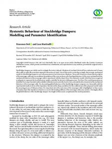
I. INTRODUCTION The objective of the research presented in this paper is to have a quadrocopter accurately track three-dimensional periodic motions, without incurring large transients at the beginning of the motion. This research is motivated by the ultimate goal of performing quadrocopter choreographies along to music. To achieve precise synchronization to a given periodic (music) reference signal, and to achieve exact reference trajectory tracking, we concentrate on adapting the parameters of the feed-forward input signal sent to the vehicle controller. An example of the 3D periodic motion considered in this paper is pictured in Fig. 1. Trajectory tracking with quadrocopters is typically achieved using feedback control approaches. Methods range from classical PID control, backstepping techniques and nonlinear control [1]–[4], to LQ optimal solutions and model predictive control, e.g. [5]. Such controllers, however, are not usually able to achieve high-performance trajectory tracking with zero phase lag for arbitrary periodic quadrocopter motions of varying angular frequencies. Perfect temporal accuracy can only be achieved by using different controllers (or controller parameters) for different motions and motion frequencies. Moreover, feedback control is inherently causal because the control actions depend only on past measurements. Causality, imperfect initial conditions and model errors effect an initial transient phase, in which the tracking errors are substantial. For choreographies in which motions are changed in quick succession, designing separate controllers for different motions is impractical, and the transient behavior as described The authors are tems and Control,

with ETH

the Institute Zurich, 8092

for Dynamic SysZurich, Switzerland.

(aschoellig,wclemens,rdandrea)@ethz.ch 978-1-4577-1096-4/12/$26.00 ©2012 AACC

Fig. 1. An example of a 3D periodic motion (with ωdx,y = 2ωdz = π rad/s, Ax,y = Azd /2 = 0.4 m, θdx = π/2). d

above is highly undesirable. Switching between different controllers may even cause instability. In this paper, we propose a control strategy that builds upon the same basic trajectory-tracking controller for periodic motions at all frequencies, but adapts the parameters of the actual input to the controller in order to guarantee precise tracking and synchronization. These parameters can be identified prior to the flight performance to effectively reduce transient time and tracking errors. Other research on motion synchronization with external inputs has focused largely on real-time interaction between robots and the environment. This research mostly deals with real-time signal processing and synchronization schemes, and typically features humanoid robots that perform rhythmic motions such as dancing, drumming and singing in tempo with an exogenous signal [6]–[8]. In contrast, our work features aerial robots and a priori known reference signals. The contribution of this paper is a feed-forward strategy that avoids the large transients, preserves the shape of the periodic motion and maintains high temporal accuracy, even in the first period of the motion. It is possible to adapt only the amplitude and phase of the motion, which is done either online, or offline prior to the actual flight performance. We show that, for directionally decoupled linear systems, the identification of offline parameters requires only a small number of experiments that can be stored concisely in a table. The general idea is based on first identifying the linear closed-loop transfer function and then using it to compensate for the steady-state errors in advance [9]. This ‘black box’ approach allows the strategy presented herein to be used for any (approximately) linear system with independent directions.

4313

V

x

V

z

z

Motion Primitive

V

Aid , ωdi , θdi , δdi

Aic , ωci , θci , δci

Periodic Trajectory Generation

sc , s˙ c , s¨c

Σ

y O x

V

y

pc , q c , rc , cc

s, s, ˙ R Online Parameter Adaptation

Identified Parameters

Trajectory Following Controller

s

Estimator

position, attitude

Cameras

Fig. 2. The inertial coordinate system O and the vehicle coordinate system V defining the vehicle attitude.

Fig. 3. The control configuration shows the online and offline motion parameter adaptation (bold boxes), and the underlying trajectory-following controller.

This feed-forward adaptation scheme was applied to quadrocopter music performances. Videos are available at http://tiny.cc/MusicInMotion. The 3D periodic motion primitives considered in this paper are presented in Sec. II. The quadrocopter dynamics and the trajectory-tracking controller are introduced in Sec. III and IV, respectively. The quadrocopter response to the motion primitives is investigated in Sec. V, where an online parameter adaptation strategy is introduced and relevant system properties are derived. The system properties are then used in Sec. VI to develop an offline parameter adaptation strategy. We show the effectiveness of the offline strategy by performing a sequence of motion primitives with a quadrocopter. Experiments are conducted in the Flying Machine Arena, an indoor test environment for quadrocopters. For a detailed description of the experimental setup, refer to [10].

which sets the motion frequencies ωdi . Ultimately, motion primitives can be arranged in a choreographic sequence and be timed to music [12].

II. PERIODIC MOTIONS We present a framework for periodic motion primitives in three dimensions, generalizing from the one-dimensional side-to-side motion in our previous work [11]. We specify motion primitives on the vehicle’s position in the inertial coordinate system O, see Fig. 2. The heading of the quadrocopter (that is, the yaw angle in Z-Y-X Euler attitude representation) is held at zero. The remaining rotational degrees of freedom are defined by the quadrocopter dynamics, cf. [10] and Sec. III. The desired position of the quadrocopter at time t, sd (t) = (xd (t), yd (t), zd (t)) is given by     x  x Ad cos(ωdx t + θdx ) xd (t) δd  yd (t)  = δ y  +  Ay cos(ω y t + θy )  , (1) d d d d Azd cos(ωdz t + θdz ) zd (t) δdz (δdx , δdy , δdz )

where is the desired center position of the motion primitive. The shape of the primitive is adjustable by a set of nine motion parameters: in each direction i ∈ {x, y, z}, we specify the desired amplitude Aid , frequency ωdi and phase θdi . By varying the nine parameters, a wide range of different motions can be expressed, such as side-to-side motions, bounces, ellipses, eights and spirals, see for example Fig. 1. Not all parameter values result in periodic motion primitives that can be followed by the quadrocopter. If the amplitudes or frequencies are too high, the motion becomes infeasible due to thrust limitations of the propellers and limited sensor range. This is investigated in [10]. The motions considered in this paper are assumed to be feasible. One of our goals is to synchronize the motion to an external reference signal (for example, the beat of a music piece),

III. QUADROCOPTER DYNAMICS The translational motion of a quadrocopter in the inertial frame O is described by       x ¨(t) 0 x ¨ = c bx 0 y¨(t) = R(t)  0  − 0 ⇔ y¨ = c by , (2) z¨ = c bz − g z¨(t) c(t) g where R(t) is the rotation matrix from the body frame V to the inertial frame O, c(t) is the collective thrust of the four propellers, and g is the acceleration due to gravity. The values (bx , by , bz ) correspond to the third column of the rotation matrix, namely (R13 , R23 , R33 ), and represent the direction of the collective thrust in the inertial frame O. The rotation matrix R evolves according to   0 −r(t) q(t) ˙ 0 −p(t) , R(t) = R(t)  r(t) (3) −q(t) p(t) 0 where (p, q, r) represent the quadrocopter angular body velocities around the body (V x, V y, V z) axes, see Fig. 2 and [13]. The quadrocopter is controlled by four inputs: a collective thrust command cc , and commanded angular body velocities (pc , qc , rc ), see Fig. 3 and Sec. IV-A. The controller design introduced below is based on the above dynamics model. For a more detailed quadrocopter model that includes rotational dynamics refer to [10]. IV. QUADROCOPTER CONTROL The overall control configuration of our approach is outlined in Fig. 3. Below we describe the trajectory-following controller (TFC) that is the basis of our approach, and analyze its properties with particular regard to periodic motions as described in Sec. II. A. Approach The TFC accepts position, velocity, and acceleration commands, denoted by sc (t), s˙ c (t) and s¨c (t) respectively, and attempts to maintain the quadrocopter on this specified trajectory. Control is based on the estimated quadrocopter position s = (x, y, z), velocity s˙ and attitude R, see Fig. 3. The TFC outputs the commands cc and (pc , qc , rc ) to the vehicle. The TFC consists of three separate loops for altitude, horizontal position, and attitude, see Fig. 4. While the TFC

4314

bx (t) = bxc (t) and by (t) = byc (t). Then, (2) can be written as

R x, x, ˙ y, y˙ xc , x˙ c , x ¨c , yc , y˙ c , y¨c z, z˙ zc , z˙c , z¨c

Position Control

bxc , byc

Attitude Control

pc , q c , rc cc

Altitude Control

b

z

Fig. 4. Cascaded control loops of the trajectory-following controller (TFC).

operates in discrete time, the controller design is based on the continuous-time system dynamics representation. The altitude control is designed such that it responds to altitude errors (z − zc ) like a second-order system with time constant τz and damping ratio ζz , z¨ = −

1 2ζz (z˙ − z˙c ) − 2 (z − zc ) + z¨c . τz τz

(4)

It uses the collective thrust to achieve this. With (2) and (4), we obtain cc = (¨ z + g)/bz . (5) Similarly, the two horizontal position control loops are shaped based on (2) with cc from (5), resulting in the commanded rotation matrix entries bxc and byc . The attitude control is shaped such that the two rotation matrix entries bx , by react in the manner of a first-order system with time constant τrp ; that is, for x: b˙ xc = (bx − bxc )/τrp . The values b˙ xc , b˙ yc are directly mapped to the commanded angular body velocities (pc , qc ) using (3) and the estimated attitude R,      1 R21 −R11 b˙ xc pc . (6) = qc R33 R22 −R12 b˙ yc Vehicle yaw control can be considered separately, since rotations around the body V z axis do not affect the above dynamics. The yaw controller is a proportional controller and the resulting yaw angle rate is mapped to rc using the kinematic relations of Euler angles. The innermost loop, on board the quadrocopter, controls the angle rates (p, q, r) to the calculated set points (pc , qc , rc ). The feedback loop closed by the TFC is responsible for maintaining the quadrocopter on a trajectory, which is provided by the periodic trajectory generation (PTG). The PTG is based on the motion primitives in Sec. II and implements (1) with motion parameters δci , Aic , ωci , θci , where the subscript ‘c’ stands for ‘commanded’. The commanded parameters are one of the following: simply the desired parameters (no adaptation); adapted online (see Sec. V); or adapted both online and offline (see Sec. VI). Fig. 3 illustrates the three options. B. Analysis To highlight the key characteristics of the above control architecture, we analyze the closed-loop dynamics under the following simplifying assumptions: (i) the commanded collective thrust can be changed instantaneously, that is, c(t) = cc (t); (ii) the estimated rotation matrix entry bz corresponds to the actual one; and (iii) we have direct control over the other two rotation matrix entries, namely

x ¨ = ux ,

with ux = fx (t, bxc ) = c(t)bxc (t)

y¨ = uy , z¨ = uz ,

with uy = fy (t, byc ) = c(t)byc (t) with uz = fz (t, cc ) = cc bz (t) − g,

(7)

where ui , i ∈ {x, y, z}, represent the flat inputs resulting from a feedback linearization [14]. Such a transformation between the virtual inputs ui and bxc , byc , cc was applied in the previous controller equations, cf. (5), allowing us to use techniques from liner feedback control design. Eq. (7) decouples the three directions and shows linear system behavior in each direction. In the ideal case where the quadrocopter dynamics correspond to the model (2), the combination of feedback linearization with velocity and acceleration feed-forward (see z˙c , z¨c in (5)) results in perfect trajectory tracking. Assumptions (i) and (ii) are good approximations due to the fast motor dynamics (with motor time constants more than six times faster than the controller time constants, cf. [15]) and due to precise attitude estimates that are based on high-accuracy camera measurements and that include a prediction step to compensate for system latencies. Assumption (iii) is true only if the system has zero rotational inertia (cf. [10]), which is not the case. In reality, exceptionally high angular accelerations (cf. [15]) can be achieved and rotational inertia terms are small. Thus, the overall closed-loop dynamics may still be expected to be approximately linear. The approximate directional independence and linear dynamics behavior is exploited in Sec. V and further investigated using experimental data, since additional effects of latencies, time discretization, on-board dynamics, and modeling errors are difficult to predict. C. Results In a first attempt, the desired periodic trajectory is directly fed to the vehicle controller (TFC); that is, sc (t) := sd (t). The quadrocopter response is a sinusoidal motion with a (after the transient phase) constant change in amplitude, phase and center position. Phase shift and amplitude error are observed in each translational direction and are not necessarily equal in size. The frequency of the quadrocopter motion corresponds to the commanded one. This suggests that the quadrocopter controlled by the TFC can be regarded as a linear system, which explains the phase offset and amplitude amplification. Fig. 5 (top figure) shows the result for a planar side-to-side motion. The amplitude error of the quadrocopter response (black solid line) is obvious, whereas the phase error between the reference trajectory and the actual quadrocopter response is hardly noticeable. In actual experiments, however, small phase errors are visible and audible when, for example, quadrocopter choreography is timed to music, as a phase shift causes a misalignment between the flight trajectory and the music beat. For the side-to-side motion, music beats may occur at the outermost points of the trajectory. In this case, humans are particularly sensitive to non-zero vehicle velocity at beat times. Correspondingly, the bottom plot of

4315

x [m]

x [m]

0.6 0 −0.6 1

2

3

4

5

6

0

1.5

2

4

6

8

10

12

14

16

18

20

2

4

6

8

10 time [s]

12

14

16

18

20

0.6 x [m]

peak vel. [m/s]

0

0.6 0 −0.6

1 0.5

0 −0.6

0 0

1

2

3 time [s]

4

5

6

0

Fig. 5. Side-to-side motion (with ωdx = 3.25 rad/s, Ax d = 0.6 m): no motion parameter adaptation. Top: quadrocopter response (solid) for a desired oscillation in the x direction (dashed). Bottom: corresponding peak velocities, i.e. absolute value of vehicle velocity at the peaks of the desired trajectory. High peak velocities imply a large phase error.

Fig. 7. Side-to-side motion. Top: online motion parameter adaptation only, quadrocopter response (solid) for a desired oscillation in the x direction (dashed). Bottom: offline motion parameter adaptation, with online motion parameter adaptation turned on after 2 periods.

Fig. 5 illustrates the velocity of the quadrocopter at beat times, i.e. when the reference trajectory reaches its maximum or minimum value. Note that if different directions exhibit different a phase shift or amplitude error, the shape of the motion primitive can even be changed, see Fig. 6. In the following section, we correct for the amplitude error and phase shift, and investigate the closed-loop behavior in more detail by analyzing the steady-state correction terms. Because the commanded amplitude is often amplified by the closed-loop system (rendering feasible commanded trajectories into infeasible quadrocopter motions), the correction is done first.

at time t. We multiply the position estimate s(t) and with the two reference signals, rcos (t) = cos(ωd t + θd ) and rsin (t) = sin(ωd t + θd ), and integrate the result over N periods, that is T = 2πN ωd . We assume that the errors stay constant over the interval [t − T, t]. This yields Z 1 t At + Ad η1 (t) = s(t)rcos (t)dt = cos(θt ) T t−T 2 (8) Z At + Ad 1 t sin(θt ), s(t)rsin (t)dt = η2 (t) = T t−T 2 and finally p At = 2 η1 (t)2 + η2 (t)2 − Ad

V. ONLINE CORRECTION

θt = − arctan (η2 (t)/η1 (t)) .

A. Approach The goal is to accurately track the desired trajectory sd (t) by minimizing the deviation from the estimated trajectory s(t). To this end, the motion parameters in the commanded trajectory sc (t) are adjusted by directionally decoupled integral controllers, see Fig. 3. The approach is based on our previous work, see [11]. For notational convenience, we drop the superscripts i ∈ {x, y, z} indicating the direction throughout this section. The motion parameters of the commanded trajectory are set to θc (t) = θd + θon (t), δc (t) = δd + δon (t),

z-position [m]

where terms. We phase

Ac (t) = Ad + Aon (t),

the subscript ‘on’ indicates the online correction They are updated in real time, during the flight. first determine the additive error in amplitude At , θt and position δt of the quadrocopter response

3.5 3 2.5 −0.6

−0.4

−0.2

0 0.2 x-position [m]

0.4

0.6

= Fig. 6. Vertical bounce motion (with = ωdz /2 = 1.56 rad/s, Ax,y d z Ad /2 = 0.6 m): no motion parameter adaptation. The vehicle’s response (solid) can differ in shape from the desired trajectory (dashed). ωdx,y

(9)

position error of the sinusoidal response is δt = RThe t (δ − s(t))dt. Since an insufficient number of meat−T d surements is available at the beginning of a motion, the integrals deliver reliable values only after several periods of the motion primitive. The online correction terms are calculated by integrating the errors according to t

Aon (t) = kA ∫ Aτ dτ,

t

θon (t) = kθ ∫ θτ dτ,

0

(10)

0

and similarly for δon (t). The gains kθ , kA , kδ are chosen to ensure converge of the online correction terms to the steadystate values θon,∞ , Aon,∞ and δon,∞ , respectively. Note again that the above online parameter adaptation strategy is implemented for each direction separately. B. Results Using the proposed online parameter adaptation strategy, the errors in amplitude, phase and center position are effectively regulated to zero, see Fig. 7. We observe a substantial transient phase before the online correction terms attain steady state, see Fig. 8. This is mainly due to the fact that the error identification scheme (8)-(9) only provides reliable values after several periods. To draw further conclusions, we consider the steadystate values in the following form: the amplitude-normalized amplification factor,

4316

i αon,∞ = (Aid + Aion,∞ )/Aid ,

i ∈ {x, y, z} ,

(11)

i i , as and δon,∞ and the steady-state phase and offset, θon,∞ before. We found that, when executing the same motion primitive multiple times, the standard deviations of the corresponding steady-state values are small. We call this the intraclass variability, which is a measure of the repeatability of the experiments. We then investigated the inter-class variability: the standard deviation of the steady-state values i i i is evaluated for different motion , and δon,∞ , θon,∞ αon,∞ primitives. We found that the inter-class variability of the obtained steady-state values for a given translational direction at a given directional frequency is of the same order of magnitude as the intra-class variability. Supported by the considerations in Sec. IV-B and by experiments shown below, this leads to the following conclusions:

•

Decoupled directions. The steady-state values i i αon,∞ , θon,∞ in each direction are independent of the motion’s components in the other directions. Moreover, as expected from the quadrocopter’s symmetry, the x and y directions exhibit the same behavior. Linear behavior. Considering the motion component in one direction i, the steady-state values depend only on the motion’s frequency in this direction ωdi . l αon,∞

Fig. 9 depicts the amplification factor and steadyi against the motion’s directional frequency state phase θon,∞ ωdi for the two directions i ∈ {x, y}. Plots are shown for ten different periodic motion primitives in 1D, 2D and 3D of various amplitudes up to 0.6 m and different relative phase shifts. The standard deviation of the steady-state terms is indicated by the vertical labels. In particular, the variability of the amplification factors translates, for the largest amplitude, to a residual deviation of ±1.5 cm, which lies within the TFC hover accuracy of ±2 cm. The variability of the phase translates to a residual time shift of ±25 ms (at maximum), which is within the human audiovisual synchrony perception limits [16], and therefore likewise negligible. These results affirm the linearity and directional independence property. Note that when performing the identification run with the same motion primitives several times, the variability is of the same order of magnitude. Consequently, we do not lose i , Aion,∞ for one motion accuracy when identifying θon,∞ primitive and later using it for another one as described in the next section. The steady-state correction terms for the center position i δon,∞ lie within the hover accuracy with a variability of i the same magnitude. Thus, the value δon,∞ cannot be called repeatable and may either be neglected because of its small average size or identified each time when flying.

0.013

0.8 x-direction y-direction mean standard deviation

0.7 0.6 0.5

0.7 0.8 0.9 1

2

3 0.030

0.1

−0.2

−0.3

0.015

0.015

0.012

0.010

0.008

−0.1

0.011

x,y θon ,∞ [rad]

0

x-direction y-direction mean standard deviation 0.7 0.8 0.9 1

•

0.012

0.009 0.010

0.9

0.017 0.025

Side-to-side motion: convergence of the online correction terms.

0.010

1

30

0.011

25

0.012

20

0.012

15 time [s]

0.014

10

0.014

5

0.012

x δon

0.014

Fig. 8.

1.1

Axon

0.015

0

x θon

αx,y on,∞ [-]

x [m] / θ [rad]

0.1 0 −0.1 −0.2

2

3

ω [rad/s]

Fig. 9. Steady-state correction values in x and y for ten different motions primitives in 1D, 2D and 3D. Here, ω = ωdx = ωdy . The vertical labels provide the standard deviation for the samples. Top: steady-state x,y amplification factor αx,y on,∞ . Bottom: steady-state phase θon,∞ .

VI. OFFLINE IDENTIFICATION A. Approach The previous section showed that the steady-state values obtained from the online correction are repeatable. Consequently, relevant steady-state values can be extracted once, and later applied to improve the transient performance. We employ offline identified parameters in addition to the online adaptation. Again, we drop the superscripts indicating the direction. The parameters of the commanded trajectory are set to Ac (t) = αoff Ad + Aon (t), θc (t) = θd + θoff + θon (t),

δc (t) = δd + δon (t),

where the subscript ‘off’ indicates the offline motion parameters identified prior to the experiment. Note that there is no offline parameter for the center point δc , because the errors are small in size and less repeatable and, thus, more efficiently handled by the online adaptation strategy. The offline parameters are selected at the start of a motion on the basis of the desired motion primitive and stay constant for the duration of the executed motion. For a given motion, the offline correction terms are set to the steady-state values obtained from the online correction, see Sec. V-B: αoff = αon,∞ ,

θoff = θon,∞ .

We make use of the directional independence and linearity property derived above to efficiently identify the offline cor-

4317

norm. peak vel. [-] error in x [m]

2

VII. CONCLUSION

without corrections with corrections

1 0 0

1.2 0.8 0.4 0 −0.4 −0.8 0

5

10

15

20 time [s]

25

30

35

15

20 time [s]

25

30

35

without corrections with corrections

5

10

Fig. 10. Sequence of motions (comprising a circular motion in 3D, a swing motion in 3D and a horizontal circle): with and without feedforward corrections. Offline correction terms were obtained from a reduced identification. Top: absolute value of velocities at the peaks of the desired x trajectory normalized by dividing by Ax d ωd . Bottom: errors between desired trajectory and vehicle response (sd (t) − s(t)) are plotted.

rection terms for all periodic motions that can be expressed in our framework (1). We perform a single identification run with fixed amplitudes Aid , phases θdi and center point δdi and vary only the frequency ωdi = ω. Moreover, since the x and y direction exhibit the same dynamics, an identification run with a 2D motion primitive in x or y, and z is sufficient to completely identify all necessary feed-forward parameters. Conceptually, the offline identification strategy results in a pair of maps x,y x,y Γxy : ωdx,y 7→ (αoff , θoff ),

z z Γz : ωdz 7→ (αoff , θoff ),

where the superscript x, y indicates that this map is used for both, the x and are stored  y direction.x,yThe values  in a x,y z z αoff αoff θoff table with rows ωdx,y ωdz θoff . We use linear interpolation between the offline parameters, which are only obtained at a discrete set of frequencies. B. Results As compared to using only online parameter adaptation, the proposed offline identification substantially decreases the transient phase, see Fig. 7. The offline parameters are effective from the start of the motion primitive. When combining online and offline correction, the former is used only after several periods. In order to show the effectiveness of the reduced identification scheme, we perform a sequence of periodic 3D motions with offline parameters obtained from an oscillatory motion in 2D (Axd = Azd = 0.4 m, ωdx = ωdz = ω). Fig. 10 shows that the quadrocopter’s deviation from the desired trajectory is clearly reduced when using the offline parameter adaptation strategy. As a consequence, the corresponding peak velocities (cf. Fig. 5) are also small indicating that the phase error is reduced. Note that the transient performance can be further improved by starting the vehicle with the appropriate velocity and acceleration. The videos at http://tiny.cc/MusicInMotion show examples of quadrocopter choreographies timed to music.

In this paper we studied a feed-forward parameter tuning strategy that improves the tracking performance of periodic motion primitives, as compared to pure feedback control, especially during transients. With pre-identified correction terms, the tracking converges to a level virtually imperceptible to a human observer within a single period. The parameter correction terms depend only on the motion’s 3D directional frequencies. The translational directions are independent, allowing for an efficient offline identification of correction values. Due to the directional independence, the approach presented in this paper can be applied even to nonperiodic 3D motions that are composed of periodic motions in each translational direction. R EFERENCES [1] S. Bouabdallah and R. Siegwart, “Backstepping and sliding-mode techniques applied to an indoor micro quadrotor,” in Proceedings of the IEEE International Conference on Robotics and Automation (ICRA), 2005, pp. 2247–2252. [2] S. Al-Hiddabi, “Quadrotor control using feedback linearization with dynamic extension,” in Proceedings of the International Symposium on Mechatronics and its Applications (ISMA), 2009, pp. 1–3. [3] T. Lee, M. Leoky, and N. McClamroch, “Geometric tracking control of a quadrotor UAV on SE(3),” in Proceedings of the IEEE Conference on Decision and Control (CDC), 2010, pp. 5420–5425. [4] D. Mellinger and V. Kumar, “Minimum snap trajectory generation and control for quadrotors,” in Proceedings of the IEEE International Conference on Robotics and Automation (ICRA), 2011, pp. 2520– 2525. [5] C. Castillo, W. Moreno, and K. Valavanis, “Unmanned helicopter waypoint trajectory tracking using model predictive control,” in Proceedings of the Mediterranean Conference on Control Automation, 2007, pp. 1–8. [6] K. Murata, K. Nakadai, K. Yoshii, R. Takeda, T. Torii, H. G. Okuno, Y. Hasegawa, and H. Tsujino, “A robot uses its own microphone to synchronize its steps to musical beats while scatting and singing,” in Proceedings of the IEEE/RSJ International Conference on Intelligent Robots and Systems (IROS), 2008, pp. 2459–2464. [7] J.-J. Aucouturier, “Cheek to chip: dancing robots and AI’s future,” IEEE Intelligent Systems, vol. 23, no. 2, pp. 74–84, 2008. [8] D. Grunberg, R. Ellenberg, I. H. Kim, J. H. Oh, P. Y. Oh, and Y. E. Kim, “Development of an autonomous dancing robot,” International Journal of Hybrid Information Technology, vol. 3, no. 2, 2010. [9] P. Allen, “Feed-forward compensated high switching speed digital phase-locked loop frequency synthesizer,” Proceedings of the IEEE International Symposium on Circuits and Systems, vol. 4, pp. 371– 374, 1999. [10] A. P. Schoellig, M. Hehn, S. Lupashin, and R. D’Andrea, “Feasibility of motion primitives for choreographed quadrocopter flight,” in Proceedings of the American Control Conference (ACC), 2011, pp. 3843–3849. [11] A. P. Schoellig, F. Augugliaro, S. Lupashin, and R. D’Andrea, “Synchronizing the motion of a quadrocopter to music,” in Proceedings of the IEEE International Conference on Robotics and Automation (ICRA), 2010, pp. 3355–3360. [12] A. P. Schoellig, F. Augugliaro, and R. D’Andrea, “A platform for dance performances with multiple quadrocopters,” in Proceedings of the IEEE/RSJ International Conference on Intelligent Robots and Systems (IROS) - Workshop on Robots and Musical Expressions, 2010, pp. 1–8. [13] P. C. Hughes, Spacecraft Attitude Dynamics. John Wiley & Sons, 1986. [14] A. Isidori, Nonlinear control systems. Springer Verlag, 1995. [15] M. Hehn and R. D’Andrea, “Quadrocopter trajectory generation and control,” in IFAC World Congress, vol. 18, 2011, pp. 1485–1491. [16] R. Arrighi, D. Alais, and D. Burr, “Perceptual synchrony of audiovisual streams for natural and artificial motion sequences.” Journal of Vision, vol. 6, no. 3, pp. 260–268, 2006.

4318