Parameter Identification for Material Models from

!" #$%" &'$( ! )*+!,.-.+ !/+(1032546 #7,' (981: * ; *+ =?@ '+(+$BAC/+DE" F*7+IG HKJ'L'MONPHKM Q MRTS UWVYX=Z\[@] ^`_[@VaX[@bdc]WeCZ f#ghjilkming`o kpcq7]rbs]ut ]&v tw [&xyVYz|{}\cbs~Om}\t!Vaq@Vac## VY{[uq7]rt{ 'kWF_[uZ\vf#5fFx3bdVa{ V CcbVa[@qub]}`w ]5l]ut ]u]u}\[@]a#\gh\h\gl]rtn]u]r}\[@]a#_v}KVYc)}\s[ubsc%n#Va[u%}\c l Y Y l FL=jlL=jR Y¡.¢£¤@¥r¦l§n¨ © ¤uª¦\£ « ¡.¬®@ªs©D®¯¦\°±¦`£l²´³=ª£ µTj¥5¶!¦`£¤uª£¨ ¨n·¹¸ºµT©r»n£ ª©Y® ¼K¡.½'¥rK·µa¤@µa¥W¢§ µT£¤@ª¿¾©D¤@ª¦\£%À%Á» µÂÃ ¤@ªs·ªÄYj¤@ªs¦`£Å½Æ¥|¦KÇÈµT· É ¡.ÊËÃFµa¥rªs·µT£¤@È=ÌC¤@ÎÍW©YÏ¨nªs®@ª¤@ª¦\£ Ð¡Ñl¨l¥|°Ò©Dµ¸ºj¤u©u» ª£ ÓÔ£ §B¢£¤uµY¥rÃF¦\È¤@ª¦\£ ÕK¡.¸ºj¤uµa¥rªsÈÖ¸º¦)§ µTÈ®°d¦`¥W³=j¥|Ó`µÑ)¤7¥|ªs£×¢£ ©D¦\·ÔÃn¥|µT®u®@ªÇ ÈsµCÌ5µT°d¦`¥|·j¤uª¦\£n® Ø ¡.½'¥rK·µa¤@µa¥W¢§ µT£¤@ª¿¾©D¤@ª¦\£ ÙK¡.ÚWµT®u¨nÈ¤@®£ §BÌCªs®@©Y¨n®u®uª¦\£n® ÛK¡¶!¦`£ ©DÈs¨n®uª¦\£ ÚWµT°Òµa¥|µa£ ©DµT® Í&Ã ÃFµT£ §nªË

x }\q7]rVY[WZ`vnzYbdVYczaVPÜ¯{Vaq@bdq&qut X=VY[@lbdq@VaÝ Þ+[Yfàß:kpcfáf#UWbsVaVY[a#Ff#%Z\w ~)]uVaXFV\Fxâfãnz`f=}`c_[@Z\vfÞ+[afäßpkpc f#5fFxybsVa{V l]rtn]u]r}\[@]a#å\tcVæ\ggh

áCq5}Ôq@]utVYc)]5Z\v']r{V6x xyáBX[uZ\[r}\3k.Zt d3dbd~`V+]rZ[uq7]+}`c3v Z\[uVa Zq7]¯]r{}\c ~B_[@Z\vf#Þ+[afäß kpc f5fxybsVa{V`v Z[{bdqzaZ\cq@]r}\c]6VYczaZt [r}\VY%VYc]Î}\c qut XX=Z\[@]TfWbdqVac]r{)tq@bÒ}\q@ }\c \tbd}`czaV {}T\VWÝFVaVYcÅ}+%} @Z[v}\zY]uZ[v Z[]u{V&qutzYzaVYquq.Z\v#]r{VWx xyá+ [u}\t}K]rVX[@Z[u}\yf`k}` V n]u[uVY%VYs [u}`]rVDv t ]rZI{bs v Z[5X [uZjlbdbscÅ V&b]r{ }`c ZXXt [@]rt cbs]p3]rZ Z[@~yZ\c 6 x}\q@]uVa[CÜ¯{Vaq@bdq}`]C]r{V kpcq7]rb]rt ]uVZ\vFá5XX dbdVYxyVYz|{}\cbszaqafk'}\E]r{ [uZt\{sPZjVY[@&{VYd VaÝÎ{bsqÆ%Z`]rbs`}`]ubdZc}\cÔ\tbd}`czaV t [ubdc ]u{VzaZt [uquVPZ\v']r{bsqZ\[u~#f kÖ!ZtsÎ}\squZWdbd~`V.]uZC]u{}\c~PÞ+[afäßpkpc fá6fKUWbsVaVY['v Z\[{bsqq@tXFVa[@lbsqubdZ\c6Z\v]u{V!]u{Vaq@bdqY!f Wbdq'"V nXÒ}`c}`]rbsZcq {VYdXFVa3%V}\bdcB}\c3bdclßpVYX ]r{B~)cZj&dVYVZ\v']r{VZX ]ubd $b #a}`]rbsZcI[uZ\t ]rbscVaq¯V X Ò}\bscVaBbdc×]u{bdq!Z[u~#f kWZt d sbd~`VÎ]rZ3"V nX[uVYquqÔ}BVYVaX q@Vacq@VÅZ\v[r}K]rbs]utVÎ]uZ å f& x VY% cV #Ix nz`'f Wbdq{VYdXº]rZj}`[uq]r{V V XFVa[@bd Vac]|}`X}\[@]&Z`v]u{VZ[@~B}\c×]r{ VPV nXÒ}\c}`]rbsZcq]r{ Va[uVYbdc3qu{}`d}\}Tlq&Ý=V[@Va VaÎÝFVa[@VaÖf kC}\ VaVaX s bscVaÝn]rVaº]rZy=fã Zw ~]rVaXFV x nz`fcZ\]Zc sv Z\[{bdqq@tX=VY[@lbdq@Z[@ tbd}\czaVÔ t[ubscI]r{V d}`]rVY[¯X}\[@]WZ\v]r{V]u{Vaq@bdqa#Ýtn]5}`dquZv Z[¯{bsq¯v [ubdVYcq@{bdXÖfk.Z\td3dbs~\V+]rZ%}\z|~)cZj&dVYV{bdq¯zYZ% bs]7ß Vac]W}\cBVYc)]u{)tqubd}\qu bscI]|}\~)bscÔZjVa[¯]u{VqutXFVa[7lbdqubsZcBZczYVÞ+[afäßpkpcfná6f UWbsVaVY[¯{}\ c bdqu{ Va3{bdq ZlzY]uZ[r}`Æq@]utbdVYqaf'xy[Yf'%Z\w ~)]uVaXF!V ( qP]ubd Vayq@tVYq@]ubdZcq{}T\V%ÝFVaVYcâV n]u[uVY%VYs {VYdX v t Æbdcº%}\~)bdc ]u{bdq!Z[u~B}Ôq@tzazYVaquqYf k+]u{}\c~O}\sÆ]r{V%zaZ`ß´Z[@~\VY[uqÎZ\v]r{V kpcq@]ubs]ut ]rV%Z\v¯á5X XdbsVa x3Vaz|{}\c bdzaqv Z[]r{VYbd[P{VasX t[@bdc3]r{V zYZt[uq@VZ`v]u{bdq!Z[u~#f áCÝ=ZjVC}\s´\k !Ztd dbs~\V]uZ]u{}\c~ÔÎX}\[@Vac]rqv Z[Æ]u{Vabs[zaZcq7]|}\c]!VaczYZt[u}\Va Vac]aflÜ¯{ Vabd[q@tXXFZ[@] bsq+&{}`]{}\qÅ}`VÎ]r{bsq}T X=Z\ququbsÝdV`fÜ¯{Vabs[zaZ)c Vac zaVÅbscº%V{}\q{VYdXFVaO%VÔ[@Va}`bdcº%bscVÎ]rZ z|{}`quVP6×[@VT}\ qaf *t bsc[ubd}\c ss]uk{V!Zt[r}`dÔtsbd}`~`]uVV]rzaZ+Z]ut{[@}\quV`cf ~}\dl6v [ubdVYcqÆZ`vF]u{V& x xyá+zYÒ}\q@qv Z[]u{Vv [ut bs]uv t nbsquzYtquq@bdZcq Ü¯{}`c~IZt+ÞÎlv Z[&}\}TlqCÝFVabscÎ]r{ Va[uV&{VYck.cVaVY-,+Pf áC[utc} _[r}\~K}\q@{

i

Contents

Contents 1. Introduction . . . . . . . . . . . . . . . . . . . . . . . . . . . . . . . . . . . . . . . . . . . . . . .

1

1.1. The Direct Problem . . . . . . . . . . . . . . . . . . . . . . . . . . . . . . . . . . . . . . .

2

1.2. The Inverse Problem . . . . . . . . . . . . . . . . . . . . . . . . . . . . . . . . . . . . . .

2

1.3. Ill-posedness of the Inverse Problem . . . . . . . . . . . . . . . . . . . . . . . . . . .

3

1.4. Motivational Example . . . . . . . . . . . . . . . . . . . . . . . . . . . . . . . . . . . . .

4

1.5. Aim of the Thesis . . . . . . . . . . . . . . . . . . . . . . . . . . . . . . . . . . . . . . . .

6

1.6. Overview of the Documentation . . . . . . . . . . . . . . . . . . . . . . . . . . . . . .

6

2. Basics of Non-Linear Continuum Mechanics . . . . . . . . . . . . . . . . . . . . .

8

2.1. Material Body . . . . . . . . . . . . . . . . . . . . . . . . . . . . . . . . . . . . . . . . . . .

8

2.2. Fundamental description of motion of the body . . . . . . . . . . . . . . . . . . .

8

2.3. Deformation Gradient: Tangent Map . . . . . . . . . . . . . . . . . . . . . . . . . . .

9

2.4. Adjoint Transformation: Normal Map . . . . . . . . . . . . . . . . . . . . . . . . . . 10 2.5. Volumetric Transformation . . . . . . . . . . . . . . . . . . . . . . . . . . . . . . . . . . 10 3. Parameter Identification - The Optimization problem . . . . . . . . . . . . . 12 3.1. General Optimization Theory . . . . . . . . . . . . . . . . . . . . . . . . . . . . . . . . 12 3.2. Optimization in 1-D . . . . . . . . . . . . . . . . . . . . . . . . . . . . . . . . . . . . . . . 13 3.3. Multidimensional Optimization . . . . . . . . . . . . . . . . . . . . . . . . . . . . . . . 15 3.3.1. Unconstrained Optimization . . . . . . . . . . . . . . . . . . . . . . . . . . . . 15 3.3.2. Solution schemes based on Newton-Type methods . . . . . . . . . . . . . 15 3.3.3. Optimization with Constraints . . . . . . . . . . . . . . . . . . . . . . . . . . 18 3.3.4. Sequential Quadratic Programming . . . . . . . . . . . . . . . . . . . . . . . 19 3.4. Exemplary Algorithms . . . . . . . . . . . . . . . . . . . . . . . . . . . . . . . . . . . . . 20 3.4.1. COBYLA method . . . . . . . . . . . . . . . . . . . . . . . . . . . . . . . . . . . 21 3.4.2. NLPQL Algorithm . . . . . . . . . . . . . . . . . . . . . . . . . . . . . . . . . . . 24 3.4.3. DONLP2 Algorithm . . . . . . . . . . . . . . . . . . . . . . . . . . . . . . . . . . 25 4. Experimental Data Acquisition . . . . . . . . . . . . . . . . . . . . . . . . . . . . . . . 27 4.1. Experimental Setup . . . . . . . . . . . . . . . . . . . . . . . . . . . . . . . . . . . . . . . 27 4.2. Specimens Employed . . . . . . . . . . . . . . . . . . . . . . . . . . . . . . . . . . . . . . 28 4.3. Optical Measurements . . . . . . . . . . . . . . . . . . . . . . . . . . . . . . . . . . . . . 29 4.4. The ARAMIS Software . . . . . . . . . . . . . . . . . . . . . . . . . . . . . . . . . . . . 30 4.5. Inhomogeneous 3D experiments . . . . . . . . . . . . . . . . . . . . . . . . . . . . . . 31

Contents

ii

5. Surface Matching and Interpolation . . . . . . . . . . . . . . . . . . . . . . . . . . . . 34 5.1. FE surface extraction . . . . . . . . . . . . . . . . . . . . . . . . . . . . . . . . . . . . . . 35 5.2. Orientation of the Measurement-Cloud . . . . . . . . . . . . . . . . . . . . . . . . . 37 5.3. Surface Matching of Three-Dimensional Surfaces . . . . . . . . . . . . . . . . . . 38 5.4. Interpolation of Experimental Data onto FE Nodes . . . . . . . . . . . . . . . . . 40 5.4.1. Linear Regression . . . . . . . . . . . . . . . . . . . . . . . . . . . . . . . . . . . 40 5.4.2. Reduced Linear Regression . . . . . . . . . . . . . . . . . . . . . . . . . . . . . 43 6. Material Models for Large Strain Incompressible Deformations . . . . . 47 6.1. Framework of Elasticity . . . . . . . . . . . . . . . . . . . . . . . . . . . . . . . . . . . . 47 6.2. Finite Linear Visco-elasticity . . . . . . . . . . . . . . . . . . . . . . . . . . . . . . . . 49 6.3. Non-linear Visco-elasticity in the Logarithmic Strain Space . . . . . . . . . . . 51 7. Parameter Identification . . . . . . . . . . . . . . . . . . . . . . . . . . . . . . . . . . . . . 53 7.1. The Least Squares Functional . . . . . . . . . . . . . . . . . . . . . . . . . . . . . . . . 53 7.2. Parameter Vector . . . . . . . . . . . . . . . . . . . . . . . . . . . . . . . . . . . . . . . . 55 7.3. Parameter Identification Tool . . . . . . . . . . . . . . . . . . . . . . . . . . . . . . . . 56 7.4. Sensitivity Analysis . . . . . . . . . . . . . . . . . . . . . . . . . . . . . . . . . . . . . . . 57 8. Results and Discussions . . . . . . . . . . . . . . . . . . . . . . . . . . . . . . . . . . . . . 58 8.1. Material 1: Elasticity . . . . . . . . . . . . . . . . . . . . . . . . . . . . . . . . . . . . . . 58 8.2. Material 2: Finite Linear Viscoelasticity . . . . . . . . . . . . . . . . . . . . . . . . . 59 8.3. Material 3: Finite Nonlinear Viscoelasticity . . . . . . . . . . . . . . . . . . . . . . 60 9. Conclusion . . . . . . . . . . . . . . . . . . . . . . . . . . . . . . . . . . . . . . . . . . . . . . . . 67 A. Appendix . . . . . . . . . . . . . . . . . . . . . . . . . . . . . . . . . . . . . . . . . . . . . . . . . 69

1

Introduction

1. Introduction Modern day infrastructure demands highly reliable structures and machine components and an efficient functionality of these systems. Very obviously, this leads to a sustained increase in the cost of manufacture. Business concerns and large organizations can illafford such cost fluctuations, which may sometimes even prove detrimental to the survival of the organization. Faced with such economic considerations, there is a huge tendency to push components and structures to their working limit. This essentially brings the reliability of these components into question. One is then forced to conduct a number of reliability tests to ensure the safe working of these components. Needless to say, this once again forces an increase in costs which is highly undesirable. Off late, there has hence been a huge thrust on Simulation Techniques to enhance system performance. The usage of simulation to substitute real time testing undoubtedly leads to a dramatic decrease in manufacturing costs. The advantages of simulation are PSfrag replacements hence manifold. This obviously leads one to question the accuracy of the results obtained by simulation. It is of paramount importance that the simulation technique used, not only provides realistic system behavior, but also provides accurate results to substantiate experimental evidence. Simulation process

True process f¯

a)

Structure

¯ u

f κ

Model

u

b) Figure 1: Illustration of True and Simulation processes

Figure 1 shows a graphical representation of a typical process. Figure 1a represents a true process. Assessment of system behavior of true structures is governed by two types of variables – the first type is the control variable f¯ representing, for instance, mechanical ¯ representing the response of the structure, loading, the second type is the state variable u for example, deflection. The assessment of engineering components and structures, or in other words, the prediction of system behavior by simulation is usually done on the basis of an assumed model. As illustrated in Figure 1b, the control variable f forms the input to the simulation, the desired output being u. The simulation is governed by the assumed model and the parameters κ governing the model. The above mentioned general principles are applicable to all engineering disciplines - dynamics, statics, fracture and damage mechanics, contact mechanics, mechatronics, nanotechnology, magnetics to mention a few. This work deals with the identification of parameters (κ) governing the simulation model, specifically with the determination of material parameters for a constitutive model. As has been obvious from the explanations thus far, an accurate simulation requires an accurate model which gives a realistic approximation of the system behavior. Restricting ourselves to the field of continuum mechanics, we hence focus on formulating an appropriate mate-

2

Introduction

rial model to realistically predict system behavior. In particular, emphasis is laid on the determination of material parameters governing the material model.

1.1. The Direct Problem To understand the concept of parameter identification, we first take a look into the structure of any Initial Boundary Value Problem(IBVP). The formulation of such a typical structural analysis is termed as the Direct problem. The solution of the direct problem leads us to the response of the system. In this approach, basic physical laws (balance laws) are postulated, supplemented by boundary conditions defining the problem. Furthermore constitutive equations relating stress and strain variables are incorporated, thus defining the material characteristics. Modern day feasibility of computing power has led to the usage of more realistic constitutive relations accounting for realistic hardening and softening behavior, rate effects, temperature effects and so on. Implicitly through the constitutive model, material parameters are introduced, summarized as vector κ ∈ P ⊂ Rnp , with np , being the number of material parameters. In this way, the mathematical formulation of the appropriate model structure, which occasionally is termed structure identification, intends to provide a qualitative description of the realistic physical behavior of the system. With this notation, the direct problem is mathematically formulated as The Direct Problem: Find u(κ,f ) ∈ U , such that g(κ,u,f ) = 0 for given f ∈ F and κ ∈ P

(1.1)

where g(κ, u, f ) = 0 are referred to as constraint conditions, which restrict the domain of the parameter vector. Through the solution of an IBVP, we determine the so-called model error emod , which is the difference in the solution of the IBVP and the actual solution. Mathematically ¯, emod = u(κ∗ ) − u

(1.2)

where κ∗ is the assumed parameter vector. If the model error is beyond acceptable limits, it is a common practice to increase the complexity of the model, which generally is accompanied by an increase in the number of material parameters np .

1.2. The Inverse Problem Contrary to the formulation of the direct problem, we formulate the problem of Parameter Identification or what is mathematically referred to as the Inverse Problem. We must understand that for the solution of any IBVP, one of the key inputs required is the vector of material parameters. In general, this parameter set is not known and must be determined on the basis of an experimental data set D 1 ∈ D. Mathematically, the formulation of the inverse problem is represented as The Inverse Problem: ¯ ∈ P, such that Mu(κ(f ,d)) ¯ =d ¯ Find κ∗ = κ(f ,d) ¯∈D for given f ∈ F and d

(1.3)

¯ which is the measurement data set, is usually regarded as incomplete and The data set d, being affected by measurement errors. Hence the resulting parameter vector κ∗ can only be regarded as an approximation to the actual parameter vector.

PSfrag replacements

3

Introduction

System

Material Model

Material Model

Control Variables

Control Variables

Material Parameters Material Pa- Initial rameters Conditions System Response

Direct Problem

System Response

System Response

Inverse Problem

Material Parameters

Initial Conditions

Figure 2: The Direct and Inverse Problem - Pictorial representation

1.3. Ill-posedness of the Inverse Problem The inverse problem of parameter identification is an ill-posed problem. Referring to the classical definitions of Hadamard [14], a problem is well posed if the conditions of (i) existence, (ii) uniqueness and (iii) stability – continuous dependence on the data – can be simultaneously satisfied. The following explanation demonstrates the violation of these requirements in the case of the inverse problem (see also Mahnken [19]). Existence During the process of performing experiments, experimental errors creep in. The source of these errors maybe human errors or machine errors. In practice these are very difficult to avoid or control. Also there is a high likelihood of limitations in the assumed model. As a consequence, the inverse problem (1.3) may not have a solution, or in other words, the exact solution of the inverse problem may be non-existent. Uniqueness The inverse problem of parameter identification usually has a great possibility of nonunique solutions. Non-uniqueness of solution poses large numerical difficulties. The presence of non-uniqueness usually indicates an under-determined system or an overdetermined system. This occurs due to the absence of certain required experimental data. For example, for an initial boundary value problem of one-dimensional elasticity, it would not be possible to determine the Young’s modulus E based on displacement data only, if E were to be a function of the geometry, i.e. E = E(x). Additional information on the forces would be very necessary. Such absence of data leads to non-unique solutions. A further example for non-uniqueness of the solution is illustrated below. Consider a stress response of a material governed by two material constants. Assuming a linear elastic law, the stress is then given by σ = (E1 + E2 ). Through experimental observation, one can determine the numerical value of (E1 + E2 ), but not E1 and E2 individually.

4

Introduction Stability PSfrag replacements

The inverse problem may not always be stable. A small perturbation in the data, someux [mm] times results uiny [mm] uncontrolled deviations of the material parameters. One must realize that these perturbations may be caused by experimental errors too. Hence experimental errors may render the inverse problem unstable. Fx [N ]

1.4. Motivational Example Mooney Rivlin model

As statedExperiment in the previous section, it is generally not possible to find an exact solution to the inverse problem defined by (1.3). What we hence seek, is a reasonable approximate to the actual parameter vector. A typical procedure to find this approximation is to construct a function using the experiment and the simulated data – the simulated data obtained through the assumed constitutive model – and to minimize this function using optimization routines. The function thus helps to compare the two data sets and the process of optimization ensures a good approximation of the experimental data by the 50 simulated data. 100 150 The usual technique of identifying material parameters is on the basis of data obtained 200 from homogeneous 250experiments. In other words, homogeneous tests such as tension, compression etc. are 300 conducted and the experimental data set is formulated. These tests are 350 then simulated assuming a suitable material model to produce realistic effects – rate 400 effects, hardening, softening etc. – to obtain the simulated data set. A least squares func450 tional is then constructed using these two data sets. Further the function is minimized in -1 the presence of constraint conditions, which define the domain of the parameters, leading -0.8 ∗ to the approximate -0.6 parameter vector κ . -0.4 -0.2 2.5

Fx [N/mm2 ]

2.0 1.5 1.0

5 10 0.5 15 20 0 25 0 30

Simulation Experiment 0.2

0.4

0.6

0.8 λ1 [−]

1.0

1.2

1.4

Figure 3: Results of Homogeneous tests on rubbery material. Simulation is done using the Mooney-Rivlin constitutive model

It must be noted here that the major goal of constitutive modeling is to obtain a model that is able to predict structural response accurately and realistically. The predictive power of the constitutive model, including the material constants, needs to be validated over a wide range of loading conditions. In other words, the constitutive model must be able to simulate real time structural behavior. To ensure this, the predictive power of the constitutive model must not be limited to/by homogeneous tests only. Inhomogeneous

5

Introduction

tests simulated with the same constitutive model must be able to predict the structural response as accurately as possible. This is because inhomogeneous tests span a wider range of loading conditions and are more closer to real time loading of a structure than homogeneous tests. Since material constants also form a part of the constitutive model, a major question hence arises – Are parameters identified from homogeneous tests also valid for the inhomogeneous case? The answer, emphatically speaking, is not always Yes. To illustrate a scenario where identification of parameters from homogeneous tests fail for inhomogeneous tests, we consider an example presented by van den Bogert & de Borst [5]. Tests were performed on specimens of rubbery materials. In the first case, homogeneous tension tests were conducted and these were simulated (ref. [26]) using the well known Mooney-Rivlin elastic model. Figure 3 illustrates the results of the identification from the homogeneous experimental results. As can be seen from Figure 3, the Mooney-Rivlin constitutive model provides a sufficiently accurate approximation of the experimental data at least in the lower load range. In view of this, one is motivated to consider the resultant parameter vector as the final vector of variables. z

y x

y z

x

PSfrag replacements

a)

b)

Figure 4: Inhomogeneous Shear tests on cuboid like specimens. a) undeformed specimen. b) Deformed model shows a clear contraction in z-direction and extension in y-direction violating physical results. Deformation plotted at ux = 20mm

However, when the same material model is used to simulate the behavior of inhomogeneous tests, contradictory results are obtained. Shear tests were performed on cuboid like specimens as shown in Figure 4a. The results of the identification process are illustrated in Figure 5. The results are obviously not very encouraging. As can be seen, the plot of Fx vs. ux does not approximate the experimental data curve correctly. What is more unrealistic is the plot of Fx vs. uy . The constitutive model predicts an extension in the y-direction, which is a completely non-physical result. Figure 4b shows the deformed mesh, which, when compared to the undeformed mesh, shows an extension in the y-direction and a contraction in the x-direction. These results are in contradiction to the experimental observations. We hence realize the need to identify parameters from inhomogeneous tests directly, as the parameters identified from inhomogeneous tests are more likely to contribute to a realistic material model. However this task is easier said than done. In the case of homogeneous tests, the least squares function which is used as a means to compare the experimental and simulated data, is formulated using state variables such as stresses. Hence maximum information is gathered from the experiment. In the case of inhomogeneous large strain problems, it is not possible to measure these state variables. As a result, the least

450 Introduction

6

-1 -0.8 -0.6 400 -0.4 -0.2 350

450 400 350

0.2 300 0.4 250 0.6 0.8 200 1.0 1.2 150 1.4 100 Fx [N ]

Fx [N ]

300

50 0 0

Simulation Experiment

5

10

15

20

ux [mm]

25

0.8 1.0 1.2 1.4 5 10 15 20 30 25 30

250 200 150 100 50


0 -1 -0.8 -0.6 -0.4 -0.2 0 uy [mm]

0.2 0.4 0.6

Figure 5: Results of Inhomogeneous tests on rubbery material. Simulation is done using the Mooney-Rivlin constitutive model. Plot of Fx vs. uy shows a non-physical result

squares functional has to modified to use the available information and the identification performed on the basis of this modified functional.

1.5. Aim of the Thesis This Master of Science thesis is titled ”Parameter Identification for Material Models from Inhomogeneous Experiments with Three-Dimensional Surface Matching”. The main aim of this work is to identify parameters from inhomogeneous models using three dimensional surface matching. The surface matching algorithm developed during the course of this work helps to map the experimental data space onto the simulated data space. The entire mapping procedure, requirement and working are discussed in the subsequent chapters. Finally, parameters for an assumed viscoelastic material model are identified, using data from inhomogeneous shear tests.

1.6. Overview of the Documentation A brief overview on the structure of the document is provided in this section. A brief introduction about the work has already been provided in this chapter thus far. Chapter 2 introduces the reader to some fundamentals of non-linear continuum mechanics. A brief look into the three basic transformations: Tangent map, Area map and Volume map is provided in this chapter. Chapter 3 deals with the formulation of optimization problem of Parameter Identification. The inverse problem of parameter identification can be solved using optimization techniques to approximate the actual parameter vector. A brief overview on the general optimization theory and classification of optimization techniques is provided in this chapter. Further, the necessary and sufficient conditions for a successful optimization are formulated. One of the common algorithms - the Sequential Quadratic Programming (SQP) algorithm - is discussed in detail. Finally, some general purpose optimization routines are discussed and a brief overview on their working is provided. Chapter 4 provides an overview on the experiments performed and the methods used to

Introduction

7

gather the experimental data. A clear understanding on the specimens involved in experimentation, the loading conditions and the complete experimental setup can be gained in this chapter. Further, usage of optical techniques to gather deformation information from inhomogeneous experiments, and the principles therein are also discussed. Chapter 5 forms the core of the thesis. A new technique of Three-Dimensional Surface Matching has been developed during the course of this work. The surface matching algorithm maps the experimental data onto the simulated data space, thereby ensuring the compatibility of the two data sets. The chapter hence deals with preparation of experimental data for the purpose of construction of the least squares functional. Finally, interpolation techniques used to gather experimental information onto the Finite Element nodes are discussed. Chapter 6 deals with the formulation of constitutive models for the purpose of simulation. Three constitutive models are discussed very briefly. A non-linear elastic model, viz. NeoHookean model and two viscoelastic models are formulated to approximate the realistic behavior of the rubbery polymer HNBR50. Chapter 7 formulates the new least squares functional for the purpose of identification from inhomogeneous data. Further it provides an overview on the identification tool/software and the structural organization of the same. Finally numerical evaluation of sensitivities for the gradient based methods is dealt with. Some numerical examples are evaluated in Chapter 8. The results obtained from the three different constitutive models assumed are discussed in this chapter. Additionally, a brief comparison of the results obtained from inhomogeneous and homogeneous parameter identification is done. Chapter 9 concludes the work with a summary. A brief outlook into certain possible future aspects of the work is also provided in this section.

8

Basics of Non-Linear Continuum Mechanics

2. Basics of Non-Linear Continuum Mechanics In this chapter, we take a look into the basics of non-linear continuum mechanics. These fundamentals are required for the constitutive modeling of materials which are later discussed in Chapter 6.

2.1. Material Body From a phenomenological point of view, a material body is defined as a physical object equipped with some physical properties like color, texture, density etc. The material body hence forms the basis for any deformation process. The material body is usually defined by a domain B in the Euclidean vector space R3 , or in other words, the body B is a set of material points P ∈ B which are mapped onto a domain B ⊂ R3 of the Euclidean vector space. R3

PSfrag replacements χ P ∈B

X∈B

y

physical body B z

x

physical body in Euclidean space Figure 6: Representation of the material body. χ maps the set of points P of the body B to the Euclidean space R3

In order to map the points onto the Euclidean space, we define a bijective map given by B → B ⊂ R3 χ: (2.1) P 7→ x = χt (P ). The bijective map assigns each material point P , at a fixed time t ∈ R+ the position x ∈ Bt in the Euclidean space R3 . For further considerations, we assume that the mappings are continuously differentiable and the inverse mappings, when required, exist.

2.2. Fundamental description of motion of the body The motion of the body maps the material points of a body onto their configurations at time t ⊂ R+ . Mathematically, it is represented by a motion function or deformation map, B → St φt : (2.2) X 7→ x = φt (X),

9

Basics of Non-Linear Continuum Mechanics PSfrag replacements φt

R3

X

x

B x

S y

z

Lagrangean Configuration Material Configuration Reference Configuration

Eulerian Configuration Spatial Configuration Current Configuration

Figure 7: Pictorial representation of the motion function. φt maps points X in the Lagrangean configuration to points x in the Eulerian configuration

mapping the material points X ∈ B onto their spatial locations x ∈ St . B and St are different manifolds in the Euclidean space R3 , which are parameterized in the neighbourhood of the material points. The Lagrangean co-ordinate is defined by X = χ(t=0) (P ).

2.3. Deformation Gradient: Tangent Map The deformation gradient is, by definition, the Frechet-derivative of the deformation map F t (X) := Dφt (X) = ∇X φt (X).

(2.3)

The deformation gradient maps tangent vectors to material curves onto tangent vectors PSfrag replacements R3

φt

Material Curve

dx

F

X

x

dX Spatial Curve

x

z

B

S

y

Figure 8: Visualization of the deformation map. F maps tangent vectors to material curves onto tangent vectors to deformed material curves

10

Basics of Non-Linear Continuum Mechanics to the spatial curves. Ft :

R3 → R 3 dX 7→ dx = F t X

(2.4)

2.4. Adjoint Transformation: Normal Map Having defined a transformation which maps tangent vectors to material curves onto tangent vectors to spatial curves, we now proceed further to define a transformation to map the normal vectors. This map, referred to as the Adjoint Map or the Co-factor Map PSfrag replacements is given by F + := det[F ]F −T = JF −T .

X x

(2.5)

This transformation maps normal vectors of material surfaces onto normal vectors of

Material Area

φt

dx1

N

da

F+ dA

R3

n

dX 2 dx2

dX 1

Spatial Area

x

z

B

S

y

Figure 9: Pictorial representation of the Normal map. F + maps normals from material configuration to the spatial confguration

deformed surfaces. F+

 3  R → R3 N 7→ n = F + N :  dA 7→ da = F + dA

(2.6)

2.5. Volumetric Transformation Finally we define a volumetric transformation. The Jacobian defined by J := det[F ] ≥ 0,

(2.7)

11

Basics of Non-Linear Continuum Mechanics PSfrag replacements

R3

φt

Material volume

dV J

dv Spatial volume

y

z

B

S

x

Figure 10: Pictorial representation of the Volumetric transformation. J maps volume elements from material configuration to the spatial confguration

maps material volume elements onto volume elements of the deformed configuration.

J:

R+ → R + dV 7→ dv = JdV

(2.8)

12

Parameter Identification - The Optimization problem

3. Parameter Identification - The Optimization problem The inverse problem of Parameter Identification deals with identification of the material parameters from the experimental data. A common classical approach for solution of the inverse problem is to consider parameter identification as an optimization problem. Typically, a least squares functional - formulated as individual distance functionals, each one relating experimental data and simulated data - is minimized in order to provide the best agreement between the experimental and simulated data.

3.1. General Optimization Theory The general optimization problem is made up of three basic ingredients: • An Objective or Cost Function, f (κ), which is to be optimized (minimized/maximized). For instance, in the case of the parameter identification problem, the objective function is the Least squares functional. • A set of parameters (κ) which control the value of the objective function - Material parameters in the case of the parameter identification problem. • A set of constraints which restricts the value of the objective function and the parameters. The constraints may be equality constraints (h(κ) = 0) or inequality constraints (g(κ) ≤ 0) Mathematically the optimization problem can be written as: f (κ) → min κ∈P

P = {hi (κ) = 0, i = 1, . . . , nh ;

gj (κ) ≤ 0, j = 1, . . . , ng } .

)

(3.1)

The set of constraints usually originate from physical conditions. In the problem of parameter identification, the constraints are generally formulated as the bounds of the parameters. Hence, a minimum of 2n constraints are obtained, n being the number of material parameters. P = {ai ≤ κi ≤ bi , i = 1, . . . , n}

(3.2)

It is to be noted here that the inverse problem is usually over-determined. In other words, the experimental data available exceeds the number of material parameters. A unique solution, hence, rarely exists. The simulated data is obtained by modeling the material behavior using a suitable constitutive model. The intricacies of the different material models used are explained in detail in Chapter 6. In order to guarantee the minimization of the objective function, we formulate the necessary conditions, which states that the gradient of the objective function must be zero. ∇κ f (κ) = 0

(3.3)

The necessary conditions ensure the existence of a local minimum κ∗ such that f (κ∗ ) ≤ f (κ) ∀κ ∈ P.

(3.4)

13

Parameter Identification - The Optimization problem Classification of Optimization methods

The general optimization problem may be classified on different grounds. Common classifications and corresponding methods are summarized in Table 1. Table 1: Classification of optimization methods based on Gradient-based, Gradient-free, Deterministic and Stochastic methods. Gradient-based Gauss-Newton Quasi-Newton SQP methods

Gradient-free Simplex methods Evolution strategies

Deterministic Simplex methods Gauss-Newton Quasi-Newton SQP methods

Stochastic Evolution strategies Monte-Carlo

Deterministic algorithms are usually of the analytical type. They are essentially sequential algorithms. These algorithms are efficient when they work at all, i.e. they tend not to evaluate functions in regions where the minima are not likely to be present. However, a disadvantage is that the method may be trapped at points which are not the global minimum. Stochastic algorithms are more generic and are very suitable for complex arbitrary cost functions. These are non-sequential random search methods. They evaluate function values at many points which are unrelated to each other. For further details the reader is referred to standard books on optimization, for eg. [1], [28].

3.2. Optimization in 1-D As a precursor to understanding optimization in multi-dimensions, optimization in 1-D, commonly known as Scalar Optimization, is studied. Optimization in multi-dimensions can always be constructed on the principles of 1-D optimization. To understand the process of optimization clearly, an arbitrary rudimentary function is considered. Figure 11 shows a 1-D function plotted against its parameter α. The final goal is to find the minimum of this function. f (α) f (αi ) + ∇α f (αi ) · sj PSfrag replacements

Area under observation

α Figure 11: Minimization of function f(α) - f(α) plotted against α

The optimization is started by assuming a feasible starting point. At this point a search direction s is devised such that proceeding along the search direction decreases the function value. It is to be noted that the exact computation of the search direction is very expensive. The complexity increases enormously with increasing dimensions and may sometimes

14


be even impossible. In such an eventuality, an approximation of the search direction is considered. There are a number of optimization strategies available. Only a brief introduction to the Bisection method and the Newton Method is given here. Some further methods are listed but not discussed. For further details the reader is referred to standard textbooks on optimization, for eg. [2], [28].

Bisection Method The Bisection method works on the assumption that there exist two values a and b such that f 0 (a) < 0 and f 0 (b) > 0. Given the interval [a, b] where the above condition is a-priori satisfied, there must exist a point ”c” such that f 0 (c) = 0. The bisection method works on repeatedly narrowing the interval until it reaches the minimum. It reduces the interval by averaging c over the interval [a,b]. If f 0 (c) < 0, then the interval is reduced to [c,b]. If f 0 (c) > 0, then the interval is reduced to [a, c]. Repetitive reduction of the interval leads the method to the minimum. Algorithm: Initialize interval [a, b] such that f 0 (a) < 0 and f 0 (b) > 0. Evaluate c =

a+b 2

and y = f 0 (c), If y > 0, then a = a; b = c = a+b 2 If y < 0, then a = c = a+b ; b = b. 2

(3.5)

Repeat steps till f 0 ( a+b )∼ = 0. 2 Newton Method The Newton method is a fast converging method and works on the principle of approximating the actual problem through a quadratic subproblem in the neighbourhood of the iteration point xk . The quadratic subproblem is obtained from a Taylor’s series expansion. f (x) ≈ q(x) = f (xk ) + (x − xk )f 0 (xk ) +

1 2

(x − xk )2 f 00 (xk )

(3.6)

The method is iterated to get a minimum. The new iteration point reads xk+1 = xk − [f 00 (xk )]−1 f 0 (xk ).

(3.7)

Of the two Methods discussed above, the Newton method is clearly fast converging. It converges with a quadratic rate to the local minimum provided that the starting point is close to the solution. The Bisection method, though simple in construction, works only in an interval where there are distinct function values which are negative and positive with the convergence rate being linear. Some further methods are Method of Golden Cut, Armijo backtracking, the Secant Method etc. For more details on these methods, the reader is referred to [32] or any standard books on Numerical Mathematics.


15

3.3. Multidimensional Optimization Multidimensional minimization is a common procedure needed in many fields. A variety of problems in engineering, physics, chemistry, etc., are frequently reduced to ones of minimizing a function of many variables. The fundamentals of optimization in higher dimensions - dimension refers to the number of parameters - can be developed from the 1-D theory itself. The given optimization problem may be written in the following form. f (κ) → min

with h(κ) = 0 and g(κ) ≤ 0

(3.8)

There is no single method that can tackle all problems in a satisfactory way. The presence of constraints, even of simple ones, increases the difficulty. It has been realized that a strategy combining different methods is able to efficiently handle a wide spectrum of problems. A few common solution strategies are briefly explained in this section. For further studies, we classify the problems into two main types - constrained and unconstrained optimization problems. 3.3.1. Unconstrained Optimization Unconstrained optimization is a relatively a simpler class of problems. As the name suggests, there are no constraints. The goal is to find a local minimizer of the cost function. Conditions for a local minimizer. For a local minimum to exist such that the descending property, (3.4), is enforced, we formulate the necessary conditions which read, If κ∗ is a local minimizer for f : Rn 7→ R, then ∇κ f (κ∗ ) = 0

(3.9)

If condition (3.9) is satisfied, we term the point as a stationary point. Additionally for this stationary point to be a local minimum, the following conditions have to be satisfied. If κ∗ is a stationary point, then κ∗ is a local minimum if and only if (iff) ∇κκ f (κ∗ ) is positive definite

(3.10)

3.3.2. Solution schemes based on Newton-Type methods The Newton-type methods for multidimensional optimization are completely based on the fundamentals described in Section 3.2. The solution scheme is an iterative scheme given by: κk+1 = κk + ∆κk = κk + αsk .

(3.11)

The increment ∆κk that updates the parameter vector κ, hence, depends on the search direction s and the step length α. The different Newton-type methods are characterized by their evaluation of the search-direction and the step length parameter. Method of Steepest Descent This method is rather simple, but shows very poor convergence especially for quadratic problems. Due to the fact that the cost function is approximated by a linear function, a

16


clear zig-zag solution scheme is observed from this method. The method proceeds in a search direction given by sk = −∇κ f (κk ),

(3.12)

which is essentially the negative gradient. The method moves along the search-direction S till it finds a minimum, and then proceeds in a direction orthogonal to the previous search-direction. It is to be noted that although two consecutive search directions are orthogonal, the method does not guarantee the orthogonality of all the search-directions with one another. The iterative solution can be seen in Figure 12(i) . Method of Conjugate Gradients In contrast to the Method of Steepest Descent, this method ensures the orthogonality of all search directions with one another. Hence the convergence is guaranteed in n steps for a n-dimensional problem. Figure 12(ii) illustrates the method for a two-dimensional problem. The search direction for this method is given by sk = −H cg k ∇κ f (κk ), T −1 where H cg (q k−1 sTk−1 ) k = 1 − (q k−1 sk−1 )

with q k−1 = ∇κ f (κk ) − ∇κ f (κk−1 ).

κ2

κ2

PSfrag replacements

PSfrag replacements κ1

  

(3.13)

 

κ1

Figure 12: Search directions of i) Method of Steepest Descent with zig-zag solution(left) and ii) Method of Conjugate gradients

Newton Method The classical Newton method approximates the cost-function through a quadratic function at every iteration point. In other words, the necessary conditions are linearized at every


17

iteration point, i.e. f 0 (κ) ≈ f 0 (κk+1 ) = f 0 (κk ) + f 00 (κk )(κk+1 − κk ) = 0.

(3.14)

The parameter update is thus given by solving (3.14). In the multidimensional context, we have κk = −[∇κ κ f (κk )]−1 ∇κ f (κk ). | {z }

(3.15)

H

A key requirement for convergence is the positive definiteness of the Hessian H.The Newton method has a quadratic rate of convergence in the vicinity of the solution. It is hence, one of the most popular methods. However the initial points need to be chosen carefully, especially in the case of non-convex problems. Quasi-Newton Method As mentioned above, a key requirement for convergence of the Newton method is the positive definiteness of the Hessian matrix H. However, the evaluation of the Hessian is a very costly affair. The basic idea of the Quasi-Newton method is to reduce this computation cost by approximating the Hessian during each iteration while retaining the positive definiteness of the matrix. There are a number of possibilities to approximate the Hessian. Some suggestions found in literature are proposals by Broyden [6], Davidon Fletcher & Powell, Fletcher [10], Goldfarb [11] and Shanno [40]. A few update suggestions are given below. For simplicity sake, the following vectorial definitions are assumed to be valid. p = κk+1 − κk

and

q = ∇κ f (κκ+1 ) − ∇κ f (κκ )

(3.16)

The simplest update is a Rank-1 update proposed by Broyden. broyden H k+1 = Hk +

(q − H k p)(q − H k p)T (q − H k p) p

(3.17)

A similar but more powerful update is the DFP-update suggested by Davidon, Fletcher and Powell. H dfp k+1 = H k +

qq T H k ppT H k + qT p pT H k p

(3.18)

A major drawback of this update is its sensitivity to the search direction. A useful and effective alternative to approximating the Hessian is to approximate the Inverse Hessaian B = [∇2 f ]− 1 directly, since this is the final requirement. A well known update sequence of B, is the BFGS-update (after Broyden, Fletcher, Goldfarb and Shanno).

B bfgs k+1

qB k q B k qpT + pq T B k ppT 1+ T − = Bk + T p q p q pT q

The BFGS update is extremely efficient and is very much in common vogue.

(3.19)

18

Parameter Identification - The Optimization problem 3.3.3. Optimization with Constraints

In contrast to unconstrained optimization, optimization with constraints defines a minimization problem for a function restricted by certain constraint conditions. The Constraint Optimization problem is formulated identical to (3.1).

f (κ) → min κ∈P

P = {hi (κ) = 0, i = 1, .., nh ;

(3.20)

gj (κ) ≤ 0, j = 1, .., ng }

In the context of constrained optimization, we formulate the dual problem or the Lagrange Problem as follows. n o with λ ≥ 0 (3.21) max inf L(κ, µ, λ) κ

µ, λ

The Lagrange functional formulates a saddle point problem which is given by nh X

L(κ, µ, λ) := f (κ) +

µi hi (κ) +

ng X

λj gj (κ) → stat,

(3.22)

j=1

i=1

where µ = [µ1 , ..., µnh ]T and λ = [λ1 , ..., λng ]T are the well known lagrange multipliers. Since the Lagrange problem encompasses the constraints too, the constrained optimization problem can be solved through one functional. Necessary Optimality Conditions For the existence of a stationary point, the Lagrange problem must satisfy the optimality conditions of the first order. If the equality and inequality constraint conditions are assumed to be linearly independent for a local minimum κ∗ of the optimization problem (3.8), then there exist a set of Lagrange multipliers µ∗ , λ∗ and the Lagrange problem leads to the well known Karush-Kuhn-Tucker (KKT) conditions for the existence of a local minimum κ∗ .

∗

∗

∗

∗

∇κ L(κ , µ , λ )

=

∇κ f (κ ) +

hi (κ∗ ) λ∗i gi (κ∗ ) ∗ λi gi (κ∗ )

= ≥ ≤ =

0 0 0 0

nh X

µi ∇κ hi (κ ) +

i=1

for for for for

∗

i = 1, .., nh i = 1, .., ng i = 1, .., ng i = 1, .., ng

ng X

λi ∇κ gi (κ∗ ) = 0

i=1

(3.23)

Thus the KKT-conditions (3.23) can be used in order to find the solution κ∗ of the optimization problem (3.20) or (3.21).

19

Parameter Identification - The Optimization problem Sufficient Optimality Conditions

A sufficient optimality condition of the second order is the positive definiteness of the Hessian Matrix of the Lagrange functional. ∗

∗

∗

∗

∇κκ L(κ , µ , λ ) = ∇κκ f (κ ) +

nh X

∗

µi ∇κκ hi (κ ) +

i=1

ng X

λi ∇κκ gi (κ∗ )

(3.24)

i=1

It hence suffices to say that if both conditions (3.23) and (3.24) are satisfied, κ∗ is a strict local minimum of the constraint problem (3.20) or (3.21). Active Set Strategy In order to handle the constraint conditions effectively, we apply the Active Set strategy. The key idea is to split the set of constraints into active (gi = 0) and inactive constraint (gi < 0) conditions. The active set A is frozen in the local iteration while determining the local minimum. gA = 0

⇐⇒

gi = 0 ∀ i ∈ A

(3.25)

The set of inactive constraints is not considered during the local iteration. However, the active set is updated after every local iteration such that the KKT-conditions (3.23) stand satisfied. 3.3.4. Sequential Quadratic Programming Sequential Quadratic Programming or SQP is one of the most efficient methods to solve Constrained Optimization problems. A very popular method, it is particularly effective in solving problems with non-linear constraint conditions. The basic idea of the SQP method is to solve the optimization problem (3.20) or (3.21) through a sequence of quadratic subproblems. With the definition of the Lagrange functional (3.22) at hand, we may reformulate the well-known KKT-conditions as follows:     ∇κ L ∇κ L (3.26) G(κ, µ, λ) :=  ∇µ L  =  h  = 0, ∇λ W L gW where the gradient of the Lagrange functional is given by

∇κ L = ∇κ f (κ) + µT ∇κ h(κ) + λTW ∇κ g W (κ).

(3.27)

The necessary conditions are evaluated by means of a Newton method. The linearization during the i-th iteration step is given by   ∆κ (3.28) G(κ, µ, λW ) + ∇G(κ, µ, λW )  ∆µ  = 0. ∆λW

Parameter Identification - The Optimization problem Using (3.26) in (3.28), one obtains the definition for the Jacobian (∇G)      n+1  κ − κn ∇κ L H ∇Tκ h ∇Tκ g W  h  +  ∇κ h   µn+1 − µn  = 0, 0 0 n gW ∇κ g W 0 0 λn+1 W − λW

20

(3.29)

with H defined as the second derivative of the Lagrange functional H = ∇2κκ L = ∇2κκ f + µT ∇2κκ h + λTW ∇2κκ gW .

(3.30)

Performing a few algebraic manipulations, one arrives at the following system of equations.  µn+1 T  2 n+1 n T  + ∇κκ f [κ −κ ]=0  ∇κ f + ∇κ h ∇ κ g W n+1  λcalW (3.31)  ∇κ h h  n+1 n  [κ −κ ]=0 +  ∇κ g W gW

Solving the above system of equations we obtain the update for the Lagrange multipliers n+1 µ = A−1 b (3.32) λn+1 W and the increment of the parameter vector. T µn+1 −1 n+1 T ∆κ = −H ∇κ f + ∇κ h ∇ κ g W , λn+1 W where A is a symmetric matrix given by ∇κ h A= H −1 ∇Tκ h ∇Tκ g W ∇κ g W

(3.33)

(3.34)

and vector b is given by

b=

h gW

−

∇κ h ∇κ g W

H −1 ∇Tκ f

(3.35)

The parameter vector is updated by the equation κn+1 = κn + ∆κn+1 . The increment of the parameter vector is usually done iteratively by the Newton method till it converges, i.e k∆κk < TOL.

(3.36)

It is important to note here that the evaluation of the Inverse of the Hessian B = [∇2κκ f ]−1 is computationally very costly and is hence approximated through the BFGS-update.

3.4. Exemplary Algorithms As indicated in table (1), optimization methods may be classified as Gradient-based or Gradient-free and Deterministic or Stochastic. We take a look into three deterministic algorithms - one Gradient-free and two Gradient-based routines. The Gradient free Algorithm (COBYLA), is based on the Simplex method and has been developed by Powell [31]. The Gradient-based algorithms – NLPQL and DONLP2 – are based on the SQP method and were developed by Schittkowski [38] and Spellucci [42] respectively.

21

Parameter Identification - The Optimization problem 3.4.1. COBYLA method

The fundamentals of working of a Simplex method can be found in Deming & Parker [8]. Nelder & Mead [27] formulated one of the earliest simplex algorithms for nonlinear unconstrained problems, which is still the method of choice for various applications. A major drawback of all gradient-based methods is the fundamental assumption that the gradient is available. In case analytical expressions for gradients are not available, the gradients are approximated through difference calculations, which could lead to a disastrous loss of accuracy. In contrast, the simplex methods do not require the calculation of gradient of the cost function. Hence they are simple in working and are known to be suitable for problems of lower dimensions. A robust simplex method was proposed by Powell [31]. Popularly known as “cobyla” - Constrained Optimization BY Linear Approximation, it is an open source tool available for free on the internet [15]. The basic idea of the simplex method - as the name suggests - is the approximation of the non-linear cost function along with non-linear constraint conditions by a linear function. A Simplex is defined as a spatial element having the minimum number of boundary points, like a triangle in 2D and a tetrahedron in 3D. To construct a simplex in a domain Rn , n + 1 points are required. For eg., to construct a simplex(triangle) in 2D, 3 points are required. The given constrained optimization problem f (κ) → min

with g(κ) ≤ 0;

i = 1, . . . , m

κ ∈ Rn ,

(3.37)

is approximated through linear simplices iteratively. The linear approximation of the cost function f (κ) is given by fˆ(κ) → min

with gˆ(κ) ≤ 0;

i = 1, . . . , m.

(3.38)

This approximation is nevertheless exact at the sampling points (vertices) of the simplex, which imposes the condition, fˆ(κj ) = f (κj ) j = 1, . . . , n + 1.

(3.39)

Further, we construct a merit function which guarantees a improvement in the shape of the successive simplices. ˆ φ(κ) = fˆ(κ) + µ[max{ˆ gi (κ), i = 1, . . . , m}]+

(3.40)

where “µ” is a parameter that is adjusted automatically and the subscript “+” means that the expression is replaced by a zero iff its value is negative. This so-called merit function also serves as a means to compare the goodness of two different vectors of variables, or in other words, the feasibility of the solution. Evidently, in the event that κ is feasible, we ˆ clearly have φ(κ) = fˆ(κ). The vertices of the simplex are ordered such that the κ(1) is optimal, i.e. the inequalities φ(κ(1) ) ≤ φ(κ(j) ),

j = 2, 3, . . . , n + 1

(3.41)

hold good. In general, this problem possesses no finite solution. Hence we define a Trust Region such that kκk+1 − κk k ≤ ρ.

(3.42)

The algorithmic formulation of the cobyla method can be split up into 3 main steps:


22

1. Formulation of the Simplex 2. Incorporating the trust-region 3. Optimization in the local iteration using the Trust radius and the merit function. Formulation of the Simplex The initial simplex is constructed using elementary perturbation techniques. The initial vector of parameters κ(1) along with the initial and final trust radii (ρbeg & ρend ) are provided by the user. We then determine the remaining n vertices of the simplex by setting κ(j) = κ(1) + ρbeg ej ,

(3.43)

where ej is the j-th co-ordinate vector. Furthermore, before proceeding to the next value of j, κ(j) is exchanged with κ(1) , iff the condition f (κ(j) ) < f (κ(1) ) is satisfied. Thus κ(1) becomes the optimal vertex of the simplex and hence, imperatively, the simplex becomes “acceptable”. The shape of the simplex changes during each iteration of the optimization process and there is a likelihood of the simplex degenerating continuously. In such an eventuality, an intermediate step is preferred which aims at improving the shape of the simplex instead of minimizing the cost-function. The current simplex would need to be revised if it is not “acceptable”, the definition of acceptable being as follows. σ (j) ≥ αρ , j = 2, . . . , n + 1, (3.44) η (j) ≤ βρ where σ (j) is the Euclidean distance from any vertex κ(j) to the opposite face of the current simplex, η (j) is the length of the edge between κ(j) and κ(0) and α&β are constants that satisfy the condition 0 < α < 1 < β. Incorporation of the trust-region In order to find an optimal solution to the problem, a trust-region is incorporated. The trust-region can be defined with the help of the the trust region radii (ρbeg & ρend ) provided by the user. The strategy is to use the current value of ρ until the iterations fail to provide a satisfactory reduction in the merit function and then ρ is decreased. In each iteration, the trust region is so formulated that it satisfies equation (3.42). It is recommended that ρbeg is set to a value which makes for a coarse exploration of the calculation, while ρend is set to a value that is approximately the distance from the final vector of variables to the solution of the optimization problem. If ρ ≤ ρend , then the iterative procedure is terminated. Alternatively, when ρ > ρend , the trust region radius is set to the value 1 ρ ρ > 3ρend 2 (3.45) ρnew = ρend ρ ≤ 3ρend .

23


If a simplex is “acceptable”, then the following condition involving the merit function is also satisfied ˆ k ) − φ(κ ˆ k+1 )], φ(κk ) − φ(κk+1 ) > 0.1[φ(κ (3.46) where φ is the merit function involving the actual cost function and φˆ is the merit function involving the linear cost function. Optimization in the local iteration Once an acceptable simplex is constructed and a trust-region is incorporated, we obtain the new set of variables κ∗ , such that the trust-region condition (3.42) is satisfied. In other words kκ∗ − κ1 k ≤ ρ.

(3.47)

If possible we let κ∗ minimize the linear approximation fˆ(κ∗ ). The new vector of variables is successively updated using the trust-region till κ(∗) no longer minimizes fˆ(κ(∗) ), then the trust-radius is updated (equation 3.45). Finally, if ρ ≤ ρend , the iterative procedure is terminated, the final vector of variables being κ(1) , except that κ(∗) is preferred instead, if φ(κ(∗) ) is available and satisfies φ(κ(∗) ) < φ(κ(1) ). Not always is the calculation of κ(∗) preferred, as sometimes it is clearly the priority to make the simplex acceptable (3.44). We then define a new vector κ(∆) that is an alternative new vector of variables that is chosen to improve acceptability. The current iteration calculates κ(∗) instead of κ(∆) if one of the following five conditions holds. 1. There is no previous iteration. 2. The previous iteration reduced ρ 3. The previous iteration calculated κ(∆) 4. The previous iteration calculated κ(∗) and reduced the merit function by at least one-tenth of the predicted reduction. 5. The current simplex is “acceptable” Exceptions can occur, however, because sometimes the previous iteration will have replaced a vertex of the simplex by the vector κ(∗) that does not satisfy (3.46). When none of the above conditions hold, the vector κ(∆) is calculated as κ(∆) = κ(1) ± γρv (l) ,

(3.48)

where v (l) is a vector of unit length that is perpendicular to the face of κ(l) . The value of l is calculated as follows: We let l be the least integer from [2, n + 1] that satisfies the equation η (l) = max η (j) : j = 2, 3, . . . , n + 1 ,

(3.49)

if any of the numbers {η (j) : j = 2, 3, . . . , n + 1} of equation (3.44) is greater than βρ.

Else l is obtained from the formula σ (l) = min σ (j) : j = 2, 3, . . . , n + 1 .

(3.50)


24

3.4.2. NLPQL Algorithm The NLPQL algorithm (ref. Schittkowski [38]) is a FORTRAN implementation of a sequential quadratic programming method for solving nonlinearly constrained optimization problems with differentiable objective and constraint functions. At each iteration, the search direction is the solution of a quadratic programming subproblem. The fundamentals of the SQP method have already been discussed in Section 3.3.4. Further details can also be found in Schittkowski [37, 39]. Only elementary details of program organization are provided here. The NLPQL sequential quadratic programming algorithm has been developed by K. Schittkowski and is distributed upon request. The program is hence a gradient-based algorithm. The program has been known to provide good results for problem dimensions of upto 100 parameters. The program is a self-sustaining algorithm. However it requires a few Fortran-routines to be supplied by the user. The user is expected to provide the subroutines FUNC and GRAD to calculate the function value and gradient of the function respectively. Most importantly, the user is expected to provide a non-linear sequential programming algorithm, a subroutine QL. Other user supplied routines are MERIT - set of active constraints and function and gradient values of the merit function, and, LINSEA - an optional user supplied routine to influence line search. The NLPQL-SQP algorithm is realized through two main subroutines - NLPQL1 & NLPQL2. These routines can be used to alter the default values provided so as to adapt the solution process to a specific situation. The most important are the following ones: 1. Alternative Subproblems: A logical variable that can be used in order to indicate whether a quadratic programming or alternatively, a linear least squares problem is formulated. 2. Expanded quadratic programming problem: In normal execution, NLPQL formulates the quadratic programming subproblem combined with an active set strategy. An additional variable δ is provided to avoid numerical inaccuracies. This additional variable is only used if the program reports an error message. 3. Scaling: Scaling is among the most difficult problems in practical optimization. Optimization problems are often posed with poor scaling, i.e. the objective function f is highly sensitive to small changes in certain components of κ and relatively insensitive in other components. Topologically, a symptom of poor scaling is that the minimizer κ∗ lies in a narrow valley, so that the contours of the objective f (·) near κ∗ tend towards highly eccentric ellipses. In general terms, one tries to achieve a model formulation such that a small fixed alteration of any variable induces an alteration of the problem functions of the same order of magnitude. A generally applicable scaling method is however not available. This is due to the fact that the nonlinear programming algorithm possesses information about the behavior of the problem only in the neighbourhood of the starting point. Although a very careful procedure is included in NLPQL, it also offers the flexibility to redefine the scaling parameters for a particular practical problem. 4. Reverse Communication: It is sometimes very helpful if the nonlinear programming code can be supplied as an auxiliary routine to facilitate reverse communication


25

- the most flexible way to solve an optimization problem. In such cases, only one iteration is performed by NLPQL1. Then the routine returns to the main calling program of the user, where new function and gradient values are evaluated. 5. Additional problem information: Initially, the approximation of the Hessian matrix is set to the identity matrix. Alternatively, the user can provide the program with his/her own guesses in order to better exploit the problem structure. The program informs the user about the termination of the algorithm, if the optimality conditions are not satisfied within some user specified tolerance. The following errors occur most frequently: – The algorithm terminates because the user-provided maximum number of iterations was attained. – The line search algorithm stopped because the user-provided maximum number of sub-iterations was exceeded. This situation usually occurs if the iterates are close to a solution but the optimality conditions can not be satisfied due to round-off errors. – The search direction sk is close to zero, but the current iterate is still feasible. The message indicates badly scaled problem functions. The program requires a core storage of approximately n2 + mn + 28n + 9m real variables, plus whatever additional storage is needed to solve the quadratic programming subproblem. The problem size is therefore limited by the core size and the capacity of the subproblem algorithm to solve large problems. 3.4.3. DONLP2 Algorithm The DONLP2 algorithm is another gradient based algorithm which is based on the SQP method. It has been developed by P. Spellucci. This algorithm is a sequential equality constrained quadratic programming method, with an active set technique. It provides for an alternative usage of a fully regularized mixed constrained subproblem in case of nonregular constraints. It uses a modified version of the Pantoja – Mayne update for the Hessian matrix(refer [30]), variable dual scaling and an improved Armijo-type step-size algorithm. Parameter bounds are treated in a gradient-projection fashion. For further details, the reader is referred to Spellucci [43, 44]. The DONLP2 program is a self-sustaining program and very user friendly. The routine may be called by using a generic call statement. CALL DONLP2 The required information about the function formulation, analytical gradient evaluation etc. are to supplied as a series of user-written subprograms. The program is very compact and is suitable for problems with 300 free parameters or less. It has an implicit implementation for the evaluation of the numerical gradients, providing three choices for the same - ordinary forward difference, symmetric difference and by Richardson extrapolation technique. The method however is limited to dimensions of 300 or less as it does not make use of sparse matrix techniques. The problem to be optimized is described through function evaluation routines. The gradient evaluation routine is an optional routine as the user may use the inherent feature


26

of numerical evaluation for the same. However, the tolerance for the evaluation of the numerical gradients have to be set through the interface routine SETUP0, which is the first routine called by DONLP2. The SETUP0 routine also helps initialize other parameters like choice of the numerical gradient type, the dimension of the problem, the constraints etc. It must be pointed out here that the SETUP0 routine supersedes the initializations already set in the main routine. A few details regarding the numerical evaluation of gradients. The type of gradient evaluation can be chosen through a parameter DIFFTYPE, with the discretization step size governed by EPSFCN. i) DIFFTYPE = 1, gradient evaluation → forward difference quotient; discretization stepsize = 0.1 EPSFCN1/2 ii) DIFFTYPE = 2, gradient evaluation → symmetric difference quotient; discretization step-size = 0.1 EPSFCN1/3 iii) DIFFTYPE = 3, gradient evaluation → sixth order approximation computing a Richardson extrapolation of three symmetric difference quotient values; discretization step-size = 0.01 EPSFCN1/7 The parameter EPSFCN is the expected relative precision of the function evaluation. The appropriate method must be wisely and judiciously chosen as numerical differentiation uses n, 2n, 6n additional functional evaluations for a single gradient for DIFFTYPE = 1,2,3 respectively. The DONLP2 routine provides comprehensive output for further evaluation through two output files. Further it also provides additional possibilities to enhance the performance of the code. Detailed information may be found in Spellucci [42].

Experimental Data Acquisition

27

4. Experimental Data Acquisition The entire process of parameter identification revolves around the construction of the Least Squares Functional (LSF), which acts as a means of comparing the experimental and simulated data. The fundamental step, is hence, to gather the experimental data. A brief overview on the techniques used to gather the experimental information is provided in this section. For further details the reader is referred to M´ endez [22], Scheday [36]. The explanation henceforth concentrates more on gathering data from inhomogeneous experiments, but the principles remain valid for the homogenous case too. Further, the experimental data obtained has to be converted into a form that is comparable with the simulated data for the construction of the LSF. This is a non-trivial issue and requires a definition of a mapping operator, the details of which are explained in Chapter 5. We proceed now to take a brief look into the experimental techniques used and the underlying principles therein.

4.1. Experimental Setup All the experiments reported in this Master of Science thesis have been conducted in the laboratory of the Institute of Applied Mechanics (Civil Engineering), University of Stuttgart. The complete details about different experimental techniques are reported in endez [22]. The laboratory offers state of the art infrastructure facilitating the exeM´ cution of 3-D inhomogeneous experiments. A universal testing machine (UTM), Franck 81815/B, manufactured by Karl Franck GmbH has been used for the purpose. The Franck machine is a UTM of the mechanical type, driven by electrical motors which allows large traverses. The nominal load for the Franck machine is 5kN. However the maximum load for any experiment performed on the machine is limited by the load of the force sensor, i.e 2kN. The experimental setup for the purpose of executing inhomogeneous experiments is shown in Figure 13. The experiments performed for this work are displacement controlled experiments. The displacement data is input through a machine control, which controls the traverse of the cross beam. Digital photographic techniques are used to gather experimental information – the displacement data of the specimen. The usage of two closed circuit digital (CCD) cameras provides for generating a three dimensional image. The cameras are connected to a computer hosting the software ARAMIS which performs the task of gathering the inhomogeneous deformation data. A force sensor (load cell) is used to determine the load of the specimen, which is then used to generate the load deflection curve of the experiment. The CCD cameras shoot pictures at regular intervals – which may be set at the start of the experiment – and pass the digital information onto the workstation hosting ARAMIS. ARAMIS then carries out the analysis of these images to generate the three-dimensional surface and proceeds further to calculate the displacement data and the strain. Two shear experiments were conducted, the details of which are explained later. For the experiment with 4mm/min, pictures were taken at intervals of 5s and for the experiment with 40mm/min, pictures were taken at intervals of 0.5s. It is important to understand the working of the two computers associated with the experiment. The first computer hosting the Franck machine controller and the second computer hosting ARAMIS software work independently of each other and do not have

28


drive screw

right CCD-camera

crossbeam

supporting beam

force sensor clamping (top)

PSfrag replacementsleft CCD-camera

specimen 2 kN

machine control

aramis clamping (bottom)

machine control

Figure 13: Experimental Setup using the Franck machine for inhomogenous experiments. The experiemental data is acquired via the force sensor and the movement of the cross beam. The left and right CCD-cameras take simultaneous pictures which are later analyzed by aramis

any link between them. Hence a problem of synchronization creeps in when one performs the experiment. In other words, during the course of an experiment, pictures from the very instant the controller begins to deform the specimen are desired. Should the first picture be taken after the Franck machine has started to deform the specimen, the three dimensional experimental results would be inaccurate. The first set of pictures would not refer to a strain free state. However, ARAMIS would proceed to assume the first set of pictures as the strain-free reference state leading to inaccurate results. To obtain synchronized pictures, we exploit the so-called holding-time of the Franck Machine, through which we apply a pre-loading onto the specimen. Both the parameters can be declared in the program governing the experiment. The holding time - by default declared to be 30 seconds - compensates for the lag between starting the experiment and the pictures taken by the cameras. This could however result in the redundancy of some pictures during the start of the experiment. These pictures may later be discarded without causing any abberations to the data obtained.

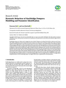
4.2. Specimens Employed For the purpose of gathering inhomogeneous experimental data, we employ hyperboloid specimens as shown in Figure 14a. Two identical specimens are used for the purpose of experimentation. However, due to symmetry, we concentrate on obtaining the optical data from only one specimen. Due to this very reason, we halve the force obtained by the force sensor. The two specimens are attached to the lower end and upper clamps and setup as shown in Figure 14b. The specimens are subjected to shearing. The main reason for the usage of two specimens is to avoid the bending moments which occur during the course of an experiment.

29

Experimental Data Acquisition 22.5

loading

PSfrag replacements

PSfrag replacements 11.8

22.5 11.8 29.3 19.3

29.3

19.3

a) b) loading a)

b)

Figure 14: Speciemen employed for Inhomogeneous Experiments - a) Model Geometry and b) Loading setup - loading of two specimens

4.3. Optical Measurements As noted in Section 4.1, we use two CCD cameras to gather the experimental data. Digital photographic techniques coupled with optical measurements are hence used to measure not only the deformation but also the geometry. The idea of using two CCD cameras is motivated by the principle of Photogrammetry. Photogrammetry is one of the optical methods which leads to the 3D-coordinates of surface points. Figure 15 shows two cameras focused to observe the same specimen or part of the specimen. The image obtained from one camera is always two dimensional. In other words, one cannot obtain the information on the depth of points from the image of one camera. In order to gather this additional information on the depth, we use a second camera, through which we correlate the data obtained from the first and hence generate information on the depth. For more information on optical measurements, the reader is referred to Bergmann & Ritter [4] and Gom [12] loading sample

PSfrag replacements Left CCD Camera

Right CCD camera

loading Supporting Beam

Figure 15: Observation of a part of a specimen using 2 Cameras to generate 3D data

It can hence be clearly concluded that measurements in 3-D space require the arrangement of two cameras - placed at an optimum angle - focused to observe the same area. A critical parameter here is the angle between the two cameras. A larger angle although enhances the accuracy of measurement, reduces the area under observation by a large extent.The maximum angle that may be used is an angle of 90◦ (Gom [12]). However the area observed

30


decreases to such great extents, that it may become insignificant. An angle of 20◦ and 60◦ is a recommended optimum angle between the cameras, especially when observing non flat surfaces. This angle between the cameras needs to be newly setup for every new experiment involving a new specimen. The reason for this is made clear through Figure 16. As can be seen, a certain shading of the observed area is caused by the placement of cameras as shown in Figure 16a. This shading of a part of the observed area is completely optical and maybe regarded as a blinding of certain areas, as a result of the geometry of the specimen, produced on either or both the cameras. The optimal placement of the cameras is thus a critical issue. A compromise must hence be made in order to achieve maximum accuracy whilst observing the maximum possible area. In other words, the experiment has to be so setup, that one is able to achieve a large angle between the cameras keeping the bounds of observation satisfactory.

a) Left camera

Right camera

PSfrag replacements

b) Figure 16: Shading of specimen: a) Blinding of a part of the specimen makes certain areas appear darker than others. b) Alternate setup to eliminate the shading of the specimen

In order to overcome the afore mentioned problem (Figure 16a), we choose an alternate setup of the cameras. The cameras are setup at an angle of 30◦ between each other. However, the entire setup is now rotated by 90◦ (Figure 16b). This not only eliminates the problem of blinding/shading of the surface, but also produces a wider image thereby gathering experimental information from a larger area.

4.4. The ARAMIS Software The application ARAMIS is used for the purpose of calculating the deformation. ARAMIS combines well known grating methods with the principle of photogrammetry to accurately recognize surface structure from digital images. The two CCD cameras produce high quality digital images which are then used by ARAMIS to allocate co-ordinates to every pixel in the image. ARAMIS bases itself on the observation of grey-scale values of a small rectangular area, also known as Facet. Deformation gradient is computed using the Adaptive Correlation method using the grey scale differences of facets. For more details on the adaptive corre-

31


lation method and further information on the working of ARAMIS, the reader is referred to Gom [12] or Bergmann & Ritter [4].

4.5. Inhomogeneous 3D experiments Data from simple shear experiments have been used in this work. The experiments were carried out by M´ endez [22] and the data has been directly incorporated into this work. Two simple shear experiments have been carried out at two different deformation rates - i) u˙ 1 = 40mm/min and ii) u˙ 2 = 4mm/min. The maximum deformation for both experiments was ±10mm. A rubbery polymer material, HNBR50, has been used for these experiments. 400

PSfrag replacements

Force[N]

200

0

−200 u˙ = 40mm/min u˙ = 4mm/min

−400 −10

−5

0 Cross Beam Position [mm]

5

10

Figure 17: Simple shear experiments at two different strain rates - u˙ 1 = 40mm/min and u˙ 2 = 4mm/min

Figure 17 shows the force deflection diagram for both the experiments. The material exhibits a clear rate dependency. It is evident from Figure 17 that a lower force is required to drive the inhomogenous specimen at a lower strain state. As noted earlier in Section 4.4, ARAMIS takes pics of the object at regular intervals while being loaded by the Franck machine. Front view

Top view

Right view

Sfrag replacements

Figure 18: Output from ARAMIS - Front, Top and right views of the observed surface in refernce configuration

32

Experimental Data Acquisition PSfrag replacements

The final output from ARAMIS is a cloud of points in the observed area of the specimen. Figurea)18 shows the calculated/output area of the reference configuration in 3D. The output is very accurate and contours the curvature of the surface very well too. This area is superimposed on the inhomogeneous specimen in Figure 19. Each point in this

time[s] ε [%]

ε [%] 1.5 1.16 PSfrag 1.18replacements 1.2 Observed Area 1.22 Figure 19: Area observed by ARAMIS superimposed on the inhomogeneous specimen used 1.24 for testing 1.26

Measurement-cloud that is output by ARAMIS contains not only information about the geometry, but also the deformation. The observed area may be regarded as rectangular with kinks on the boundary. However the boundary of the observed area is not constant. 600 Experiment

2 3

−1 −0.75 0.5 −0.25

400 1 4

200 F orce[N ]

P11

L E [N/mm2 ]

10

5

0 9

6

−200 25 75 −400 80 90 100 125 −600 150 175

8

−20

7

−15

−10

−5

0

5

10

15

20

Cross − beam position [mm]

Figure 20: Load deflection curve of experiment with u˙ = 40mm/min with corresponding specimen positions.

Figure 20 and 21 show the results of the experiment with u˙ = 40mm/min. Each picture of the surface in Figure 21 corresponds to a deformation state shown in Figure 20. As

1.26 600 400 200 0 Experimental Data Acquisition 33 −200 −400 −600 can be−1seen clearly, starting from the reference configuration 1, there is a rapid change in −0.75 the boundary with every deformation step (Figure 21), with the same boundary as the reference configuration being obtained at steps 5 and 10 which correspond to a zero 0.5 load position. Picture 2 is the deformation half way through to the maximum positive −0.25 −20 −15 −10 −5 0 5 10 15 20 25 75 80 90 100 125 150 175 Figure 21: Changing of surface boundary with change in deformation state. Each picture corresponds to the respective state shown in the load deflection curve

deformation of 10mm. Picture 3 refers to the maximum positive deformation of 10mm. Picture 4 refers to a configuration half way from the maximum deformation state encountered during unloading of the specimen. Due to a viscous behavior of the material and the prevalent hysteresis, the zero strain state is obtained only in picture 6. Pictures 7,8,9 are analogous to pictures 2,3,4 but with the specimen being loaded towards a negative maximum deformation of 10mm. The contours in Figure 21 are the contours of the shear angle. For more details on the shear angle, the reader is referred to M´ endez [22] and Gom [12]. This change in boundary in every step of the deformation process is a undesirable and unpleasant feature. This leads to a change in the observed area with every step of the experiment. When it comes to identifying parameters from the experiment, it would necessarily mean that the comparison of experimental and simulated data is not the same for the entire load cycle. Further the changing boundary also poses problems in the Surface Matching Algorithm discussed later in Chapter 5. Hence special care has to be taken to compensate for this boundary change and ensure consistency throughout the entire cycle.

34

Surface Matching and Interpolation

5. Surface Matching and Interpolation A key requirement to the construction of a functional (Least Squares Functional) to compare the experimental and simulated data is the existence of the experimental data (uexp ) in a format comparable with the simulated data (usim ). In simple words, the experimental data is required at exactly the same points/nodes where the simulated data is available or vice versa. However this is usually not the case. Needless to say, the experimental and the simulated data must also refer to the same physical quantity. The experimental and simulated data however belong to two different vector spaces U exp and U sim respectively, such that uexp ∈ U exp

and

usim ∈ U sim .

(5.1)

Generally, the two vector spaces are not directly comparable as U sim ⊂ / U exp . Hence the experimental data needs to be mapped on to the simulated vector space. Mathematically, we define a mapping operator M such that Muexp (κ) ∈ U sim .

(5.2)

The usual technique to accomplish this mapping is to interpolate/extrapolate the experimental data onto the Finite Element (FE) nodes. The experimental data is gathered through optical techniques, the details of which are explained in detail in Chapter 4. The two-camera technique provides for a three-dimensional view to be obtained. It is to be noted however that, only a part of the entire specimen is observed. The data obtained pertains to a cloud of points which corresponds to a part of the surface of the specimen under observation. Data pertaining to an interior material point is not available. Added to the above, the experimental data space is a very small subset of the complete data space because data pertaining to a very small part - small part being only a part of the surface - is obtained. This is further complicated by the fact that the experimental and simulated data exist in totally different cartesian co-ordinate systems. What is hence required, is a technique to extract those FE nodes from the complete FE mesh that correspond to the Measurement-cloud obtained through optical measurements and interpolate the experimental data onto the FE nodes. A 3-D Surface Matching technique was developed during the course of this work to accomplish the fundamental requirement of gathering the experimental data onto the FE nodes. The mapping of the experimental data space onto the simulated data space is performed in the following steps: 1. Extraction of the FE surface corresponding to the measurement data points. 2. Orientation of the measurement co-ordinate system to roughly match the FE coordinate system. 3. Matching of the FE and Measurment surfaces. 4. Interpolation of experimental data onto FE nodes.

35


5.1. FE surface extraction The Finite Element (FE) mesh of the inhomogeneous specimen has been modeled using ANSYS FE package. Figure 22a shows a simulation model of the specimen. The basic geometry of the inhomogeneous specimen is shown in Figure 24. The specimen is modeled on a hyperboloid, which clearly gives a inhomogeneous deformation, especially under shear. The model consists of 1463 nodes and 1152 elements. A figure of the measurement data points or what is further referred to as the Measurement-cloud, obtained from optical measurements is shown in Figure 23. Only the surface nodes of the FE mesh which correspond to the Measurement-cloud are to be extracted. Area corresponding to the Measurement cloud

PSfrag replacements

b)

a)

Figure 22: Simulation model of the specimen - Finite element mesh

Prima Facie, the bounds of extraction are determined from the extremum of the Measurement-cloud. What is finally required are the surface nodes from the complete FE mesh which are inside the rectangle shown in Figure 22b. As easy as it may seem, the task becomes complicated due to the approximation of the curvature of the hyperboloid in the FE mesh. It is important to note here that the simulated vector space (U sim ) PSfrag replacements consists of only these points which are referred to as the FE surface. However, the FE computation is to be made for the entire specimen and the data pertaining only to the FE surface needs to be extracted. Hence it suffices to say that although a finer mesh may provide not only for a better approximation of the curvature, but also for sufficiently accurate simulated data, the cost of computation of the simulated data increases enormously. Hence care needs to be taken in choosing the mesh so that a proper balance is created in approximating the geometry and computational effort. 8 4 0 -4 -8 -12 -16 -20 -15 -10

-20 -5

0

5

-24 10

15 -28

Figure 23: Measurement cloud - Cloud of points output from aramis

36


To extract the FE surface from the complete FE mesh, we exploit the fundamental rules of analytical geometry. We know that the general equation of a circle with center (x 0 , y 0 ) is given by (x − x0 )2 + (y − y 0 )2 = R2 ,

(5.3)

where R is the radius of the circle and (x, y) is any point on the circumference. 22.5

PSfrag replacements 11.8 19.3

29.3 z

x ¯ Figure 24: Specimen model geometry - All dimensions in mm

We consider an imaginary plane of reference, called the x¯ − z plane, along the x − z plane. The curvature of the hyperboloid corresponds to a circle of radius 11.8mm as shown in Figure 24. With this basic knowledge at hand, we extract all the surface nodes of the FE mesh through the equation (¯ x − x0 )2 + (z − z 0 )2 = R2 , (¯ x − 29.3)2 + (z −

19.3 2 ) 2

= R2 .

x¯ is the pseudo x co-ordinate given by the well known Pythogoras equation p x¯ = x2 + y 2 ,

(5.4)

(5.5)

and acts as an imaginary x-coordinate for any point in the specimen. x¯ is representative of both the x and y co-ordinates of any FE node. Since the curvature is approximated in the FE mesh, (5.4) is relaxed to an inequality within a certain tolerance (TOL). k(¯ x − 29.3)2 + (y −

19.3 2 ) − R2 k ≤ TOL 2

(5.6)

The important task of extracting all the surface nodes from the complete FE mesh has been accomplished thus far. What remains is the task of extracting only those nodes from the complete set of suface nodes, that correspond to the Measurement-cloud, which is a trivial task given the bounds of the Measurement-cloud. Once the bounds for the surface nodes are set, the FE nodes which correspond to the Measurement-cloud are extracted. The obtained FE surface (Figure 25) corresponds, in its geometry, to the Measurement-cloud. It must however be noted that the extracted FE surface and the Measurement-cloud are likely to have different orientations and may exist in different cartesian co-ordinate systems.

PSfrag replacements

37


14 11 8 5 -12 -14 -15 -10

-5

-16 0

5

10

15 -19

Figure 25: FE surface - FE nodes corresponding to the Measurement cloud extracted from the complete FE mesh

5.2. Orientation of the Measurement-Cloud As stated earlier in Section 5.1, the FE surface and the Measurement-cloud are, more often than not, oriented in different directions. The task of matching the two surfaces in order to interpolate the data from the Measurement-cloud onto the FE nodes can only be performed, if the two surfaces are oriented in the same direction. The direction of orientation refers not only to the orientation of the surface normals, but also to the deformation. Figure 26 shows the hyperboloid specimen with its axes orientations in experiment and simulation. Both are cartesian co-ordinate systems. However, the differences in the orientations can be clearly visualized. The surface normal of the simulation model is oriented in the negative y-axis direction, while the surface normal of the measurement model is oriented in the positive z-axis direction. Further, the base of the simulated model is fixed, in contrast to the measurement model, where the top of the specimen is fixed. This could probably be avoided by choosing to perform the experiments with a correct setup and the right boundary conditions, or choose the simulation so as the simulate the experimental boundary conditions. However due to some unforeseen circumstances, this may not be possible. In such circumstances, orientation of the Measurement-cloud and the FE surface in the same directions becomes inevitable and must be performed. Fixed at the Top

y

z

PSfrag replacements

x

(a)

(b)

x Fixed at the Base

Figure 26: Axis orientation of the specimen in (a) Experiment and (b) Simulation

Care must also be taken that the deformation directions are the same in both the cases. If the orientation of the deformation direction is not taken into account and the surface matching and interpolation is proceeded with, then the measurement values obtained by interpolation would never concur with the values of the simulation.


38

For the specimens shown in Figure 26, a change in the axes of the measurement specimen would be enough to orient the normal in the right direction. However, since the boundary conditions also need to be taken into consideration, the y-axis needs to be inverted. The algorithm to orient the specimens in the right direction is summarized in Table 2. Table 2: Algorithm for Orientation of the two Surfaces

Algorithm Step1: Invert y-axis of the measurement specimen, i.e. make y = -(y). =⇒ This changes the boundary condition of the measurement specimen to base fixed. Step2: Continuing with the specimen obtained from Step 1, i) Make y-axis as the new z-axis ii) Make negative z-axis as the new y-axis.

What is finally obtained are two surfaces which have their surface normals oriented towards the same octant, which forms a pre-requisite to matching the two surfaces.

5.3. Surface Matching of Three-Dimensional Surfaces Surface matching signifies a very important step in the process of experimental data acquisition onto the FE nodes. A typical procedure to gather the experimental information onto the FE nodes is to interpolate the experimental values onto the FE node. The minimum information required to perform interpolation is knowledge about the data points from which information needs to be gathered to interpolate. Unfortunately, this is a-priori unavailable. Hence a technique needs to be developed, which would help identify the points from which data can be interpolated. The process of surface matching matches the three dimensional surfaces obtained from the finite element mesh and experiment. This is an ideal solution, as the matching of the two surfaces would result in the two surfaces sharing the same co-ordinate space whence the points, from which interpolation can be performed can be identified very easily. The implementation of the matching of the surfaces is motivated from the physical background of the two surfaces. We do not have much information about the two surfaces. However, observing the physical existence of these two surfaces, we deduce that these two surfaces refer to the same part of the inhomogeneous specimen. Since the two surfaces are the result of two different processes, the data points have different co-ordinate locations. As a result, a rigid body translation of the measurement surface would be sufficient enough to match the same with the FE surface. With this physical motivation in view, we proceed with performing the rigid body translation of the measurement surface. A function representative of the distances between the two surfaces is constructed. The function is then minimized using optimization techniques. Minimization of the function results in nullification of the distance between the two surfaces, thereby matching the two surfaces. At this point, the inaccuracy in approximation of the curvature of the FE surface needs to

39


be mentioned. As mentioned earlier, a coarse mesh results in a bad approximation of the curvature. This also leads to a problem during surface matching. Although, theoretically speaking, the distance between the two surfaces is zero after matching, this would never be possible due to the approximation of the curvature of the FE surface. A question as to whether the curvature of the measurement surface is approximated, arises at this PSfrag replacements context. Hence, it is worth a mention that the optical techniques profile the curvature of the measurement surface very accurately. We therefore, assume the curvature of the measurement surface to be the actual curvature of the specimen.

r7min r1min

1

7 r6min 6

r2min

2

r5min

r3min

Measurement surface

5 3

r4min

4 FE surface

Figure 27: Simulation model of the specimen - Finite element mesh

The numerical implementation of this method involves minimization of the minimum distance between a FE node and the Measurement-cloud, whilst regarding these points to be an integral surface. To understand this concept of minimum distance between a FE node and the Measurement-cloud, we refer to Figure 27. For every FE node, we calculate the distance between the FE node under consideration and every measurement data point. We then choose that measurement point which has the least distance to the FE node under consideration and designate the distance as rimin , where the index i denotes the number of the FE node. Finally the cost function is constructed by summing up all the minimum distances. If nfe represents the total number of the finite element nodes, then the cost function may be mathematically represented as f=

nfe X

rimin → min.

(5.7)

1

This construction of the cost function, though very primitive, neglects the curvature of the surfaces, thereby reducing considerable risks. Some salient features of this surface matching technique are mentioned below i) The matching of the two three-dimensional surfaces is always carried out in the Lagrangean configuration. ii) The Measurement-cloud is preferably required to be a static set. In other words, the set of measurement points which exist in the Lagrangean configuration must exist in all the Eulerian configurations which are under consideration. This may seem unnecessary considering the fact that we match the surfaces in the Lagrangean


40

configuration. However, when the experimental information is interpolated onto the FE nodes, it is mandatory that the interpolated value for each FE node is determined from the same set of experimental data points, otherwise the interpolated value would be determined from different set of points and may not be accurate enough. Further details to this are explained in Section 5.4. iii) The method works on the presumption that the statistical distribution of the measurement points is high. This is required because of the primitive cost function formulated to represent the distance between the two surfaces. A statistically high distribution of the measurement points would implicitly account for the curvature. Also, preliminary studies suggest that insufficient data points is likely to cause a lateral shift. The lateral shift was found to be the minimum distance between two measurement data points. Hence a high resolution of the measurement points would reduce this lateral shift, thereby increasing the accuracy of the results obtained. iv) The Surface matching problem is an ill-posed problem. The problem is more profound when the resolution of the measurement points is low. This leads to a further problem during the process of optimization. The optimization routines minimize the function to a local minimum and re-optimization fails to generate a better solution. A statistically high resolution of the Measurement-cloud is a must for the Surface Matching Algorithm to conclude successfully. v) The Surface Matching Algorithm works on the assumption that the two surfaces being matched are actually the same. In essence, the normals of the two surfaces must be oriented in roughly the same direction. This must be ensured before the surfaces are actually matched. Figure 28 depicts the Surface Matching Algorithm pictorially. The initial positions of the two surfaces are shown in Figure 28a and 28b. Figure 28c and 28d shows the final position of the two surfaces after they are matched correctly, i.e the function is minimized to a global minimum. In case the function is optimized to a local minimum, it results in a vertical shift which is visually recognizable - Figure 28e 28f. Animations of Figure 28 to visualize the Surface matching procedure are made available on the website of the author [17].

5.4. Interpolation of Experimental Data onto FE Nodes The final aim of this mapping procedure or Surface Matching algorithm is to gather the experimental information from the Measurement-cloud onto the finite element nodes, so that a least squares functional which compares the experimental and the simulated data can be constructed. So far, we have been successful in gathering the experimental data (Chapter 4) and matching the two three dimensional surfaces. We now proceed to interpolate the experimental values from the Measurement-cloud onto the FE nodes. 5.4.1. Linear Regression The first obvious and simple choice for interpolation is to proceed with a linear regression fit. For a linear regression fit in n-dimensions, we require n+1 points. Hence in 3-D, we require four points to construct a tetrahedron, from where we may proceed with the interpolation. Intuitively, for each FE node, we choose the four nearest measurement points. Since we deal with inhomogeneous deformation in this work, the experimental

(c) -10 (d) -15

(c) -20 -10 (d) -24 -15 (e) -28 15

(f) 20 15

Surface Matching and Interpolation 10 5 15 Measurement Cloud FE Mesh

0 -5 5 -10

15 -15 -12 10 -20 0 5 -16 20 -5 0 -5 15 -10 -24-10 10 -15 -28 5 20 -20 -15 -10 0 -5 15 -5 10 -10 Front View 5 -15(a) 0

-12 -16 -20 0

5 10 -28 15

10 18 5 14 0 15 -5 10 -10 5 -15 6 -20 2 -12 0 -16 20 -5 -20 -10 -24 -15 -28 15

41

Measurement Cloud FE Mesh 15 10 5 0 -5

10

-24

5 0 -20 -15 -10 -5

0

5

10

15

-10 20

(b) -15 -5 -10

-5

-15

-10 -15 -12 -20 -1618 20 14 1510 -24 10 6 -28 5 2 20 0 15 -20 -15 -10 -5 10 5 (c) 0

Measurement Cloud FE Mesh


-20 -12

20

-16 -20

15

-24 10

-28

5

-5 -10 0

-5

-15 5 10 15

-20

-10 -20 -15 -10 -5

0

5

10

15

0 20

-15(d)

-5 -10


-15

Measurement Cloud FE Mesh 20

-20 18 2014 1510 10 6 5 2

15 10 -5

0 -20 -15 -10 -5 (e)

-10 0

-15 5 10 15

-20

5 -5 -10 -20 -15 -10 -5

0

5

10

15

0 20

-15(f)

Figure 28: Surface Matching Algorithm - (a): Initial positions of the FE mesh and Measurement cloud (3D view); (b):Front view of (a); (c) Matched surfaces in their final positions - Correct Matching (3D view); (d) Front view of (c); (e) Incorrectly Matched surfaces optimization to a local minimum; (f) Front view of (e) - Note the vertically unsymmetric placement of the FE mesh in the Measurement cloud

information required is displacements. We compute the displacement values of each FE node based on the values from the four nearest measurement points through the equation,       1 dx a0x a1x a2x a3x    dy  =  a0y a1y a2y a3y   x  (5.8)  y  dz a0z a1z a2z a3z z

42

Surface Matching and Interpolation or in short d = A xfe ,

(5.9)

with xfe −→ [1 x y z]T where [x y z]T are the co-ordinates of the FE node A −→ Interpolation Matrix d −→ Interpolated displacement values for the FE node. The interpolation matrix A is determined from the basic rules of linear regression in three dimensions. For further explanations we denote A as a vector:  t  ax A =  aty  = atα (5.10) t az with

 a0x  a1x   atx =   a2x  a3x 

 a0y  a1y   aty =   a2y  a3y 

The vector A is obtained from the equation G atα = dmes α

 a0z  a1z   atz =   a2z  . a3z 

with α = x, y, z,

where the matrix G is a matrix of the co-ordinates of given by  1 x 1 y1 z1  1 x 2 y2 z2 G :=   1 x 3 y3 z3 1 x 4 y4 z4

(5.11)

(5.12)

the four measurement data points    

(5.13)

and the vector dmes is a vector of the displacements of the four measurement data points, α   dα1  dα2   dmes = (5.14) α  dα3  dα4

with α signifying one of the three cartesian directions [x, y, z].

This method is very simple and easy to use. However this method has a few limitations. i) The problem is ill-posed. As a matter of fact, Quarteroni, Sacco & Saleri [33] suggest that the problem of finding an interpolating polynomial of degree n in d dimensions, with d ≥ 2, given n + 1 nodes might be ill-posed. Needless to say, the displacement values obtained at certain points were found to be totally incorrect. ii) Choice of four nearest measurement points for each finite element node does not necessarily guarantee the existence of the FE node inside the volume constructed by the measurement points. This violates the fundamentals of interpolation. iii) The aspect ratio of the tetrahedron constructed from the four measurement points plays a very important role. In some cases, the tetrahedron degenerates and hence the aspect ratio also deteriorates and this leads to very inaccurate results.

43

Surface Matching and Interpolation 5.4.2. Reduced Linear Regression

Given the above limitations of the linear regression method (Section 5.4.1), we formulate a new method to proceed with the interpolation. This technique is completely based on the linear regression, however, instead of the previous interpolation in three dimensions, we perform the same in 2-dimensions. This is motivated from the fact that although the two surfaces exist in a 3-D cartesian co-ordinate system, the surfaces are actually two dimensional, i.e. they lack thickness. Hence we can proceed with using the 2-D regression formulae. However this requires a change in co-ordinate system. A complete change of the co-ordinate system from a cartesian system to a cylindrical or a spherical system is not advisable due to two main reasons. Firstly it is computationally very costly and second, due to the inaccuracies in the approximation of the FE surface, the constructed co-ordinate system may not be accurate enough. Hence we proceed by changing the co-ordinate system only locally for every FE node. In what follows, this is made more clear. The term Reduced is used to signify a local decrease in dimension to counter the ill-posedness of the linear regression fit. In contrast to linear regression in 3-D, we choose 3 nearest measurement points for each FE node. We proceed by creating a local co-ordinate system using these 3 points. Figure 29 gives a clear picture on the co-ordinate system. If p1 , p2 , p3 are the three nearest ut y

p3

PSfrag replacements

p0 k p

n v

u p1

p2 x

z Figure 29: Projection of the FE node (p0 ) onto the local (u − v − n) co-ordinate system

points, then we define u := ut

p1 − p 2   kp1 − p2 k 

p3 − p 2   := kp3 − p2 k

,

(5.15)

44

Surface Matching and Interpolation with  p1x p1 =  p1y  p1z 



 p2x p2 =  p2y  p2z



 p3x p3 =  p3y  . p3z

(5.16)

We note that the two vectors are normalized. The vectors u and ut define a plane. The normal to this plane can be determined by the cross product of these two vectors. n=

u × ut ku × ut k

(5.17)

To define an ortho-normal co-ordinate system, we require three orthogonal vectors. Since the orthogonality of u and ut cannot be guaranteed, we define a vector v, which is determined by v=

n×u . kn × uk

(5.18)

u, v and n now define an ortho-normal cartesian co-ordinate system. If n := [nx , ny , nz ]T is the normal to the plane formed by u and v, the equation of this plane Λ is given by Λ := nx x + ny y + nz z + dpl = 0,

(5.19)

where [x, y, z]T = pg is any point on the plane. If pg is not on the plane, then the equation results in a non-zero value. If this non-zero value is positive, then the point is above the plane, otherwise it is below the plane. Since p2 is a point on the surface, we calculate dpl of (5.19) by dpl = −(n · p2 ).

(5.20)

If p0 is the finite element node, then the normal distance k of the FE node to the plane is given by k = (n · p0 ) + dpl .

(5.21)

We proceed further by projecting the FE node onto the plane formed by u and v. The projected point p is given by p = p0 − kn.

(5.22)

What is now required is to express all co-ordinates in the local co-ordinate system, so that the displacement values can be interpolated onto the FE node. To this extent we define a matrix B.  T  u  B := v T  (5.23) nT

In what follows the subscripts u and v denote the components of the vectors in the local u − v − n co-ordinate system and the subscripts x, y and z denote the components of

45


vectors in the global x − y − z co-ordinate system. The local co-ordinates of the points p1 , p2 , p3 are determined by the equation, Bq i = (pi − p2 );

i = 1, . . . , 3

(5.24)

and the local co-ordinates of the projected point are determined by the equation, Bq = (p − p2 ).

(5.25)

Having reduced the dimension of the problem from three to two, we now proceed with the actual interpolation. We proceed in the same steps as outlined in Section 5.4.1. Analogous to (5.13), we define the G matrix in the local co-ordinate system by   1 q1u q1v G :=  1 q2u q2v  . (5.26) 1 q3u q3v The displacement vector dmes is defined by α   dα1 d =  dα2  with α = x, y, z, dα3

(5.27)

which is completely analogous to (5.14). We proceed to evaluate the interpolating coefficients through the equation G atα = dmes α

with α = x, y, z.

(5.28)

The interpolation matrix A is then constructed as per (5.10) with the final matrix reading   t   ax a0x a1x a2x (5.29) A = atα  aty  =  a0y a1y a2y  . t a0z a1z a2z az The displacements of the FE node are now determined by the equation,        dx 1 a0x a1x a2x      dy  =  a0y a1y a2y   qu   dz a0z a1z a2z qv      d = A q fe

(5.30)

The displacements obtained from the above equation are actually the displacements interpolated onto the projected FE node and not the actual FE node itself. However, the values obtained from (5.30) are assumed to be the values of the actual FE node.

The justification for such an assumption comes in view of Section 5.3, where the distance between the Measurement-cloud and the FE surface has been reduced to a minimum. During the process of interpolation, in this work, the maximum distance between any FE node and its corresponding projected point was found to be 1/20th of the minimum distance between two FE nodes, which is negligible.

Sfrag replacements

46


Perform experiments on inhomogeneous specimens Extract nodes from FE mesh corr. to the measurement cloud/observed area

Obtain data from expt. with help of ARAMIS

Construct cost function

f :=

P

r min i

Initialize the movement vector dx = dx0

Minimize cost function (Optimize) to match the surfaces

Verify the obtianed result → Satisfactory??

No

Yes

Interpolate Disp. values onto FE node

END

Figure 30: Flowchart summarizing the Surface Matching Algorithm

A flowchart summarizing the entire Surface Matching Algorithm discussed thus far is shown in Figure 30. The algorithm has been programmed in Fortran77 ([9]) and optimized for better performance ([23], [24], [16]). A short note on the procedure described so far to gather the experimental information. The 3-D Surface Matching Algorithm is not a fool proof algorithm. As mentioned in Section 5.3, the function has a tendency to be minimized to a local minimum. Hence visual verification is very necessary before one proceeds to use the interpolated experimental results for parameter identification. Studies during the course of this work have shown that this optimization to a local minimum is clearly visible as shown in Figure 28 (e) & (f). In order to minimize the distance between the two surfaces, better function, which takes the curvature of the surfaces may be constructed, or a function which is constructed through planar equations defined for each surface may be used. This not only reduces the risk of optimization towards local minima, but would also provide better and accurate results. Also, better interpolation techniques which use more than 3 measurement points may be used, so that the experimental information is better approximated.

47

Material Models for Large Strain Incompressible Deformations

6. Material Models for Large Strain Incompressible Deformations Assumption of accurate material models to simulate the experimental behavior is one of the key concerns in Parameter Identification. More often than not, precious time and effort is spent in deciding on the right material model(s). It is surely a paradox that the same material model along with the material parameters determined through the exercise of parameter identification would later be used to accurately determine the behavior of real structures, which makes the effort of constitutive modeling all the more significant. Having said that, assumption of an accurate constitutive model for new materials is no mean job, the complication being enhanced in the case of inhomogeneous deformations. In this section, an effort has been made to look into constitutive modeling for rubbery polymers, in particular, for the material HNBR50.

6.1. Framework of Elasticity Rubbery polymers clearly exhibit inelastic (viscoelastic) deformations. However as a precursor, we study the framework of non-linear elasticity(Ogden [29]). This, additionally serves two main purposes during the process of parameter identification. Firstly, the identified elastic material parameters provide a good starting value for the inelastic framework. Secondly, this framework may also be used to verify the least-squares functional and the optimization routines used. PSfrag replacements λ2

λ3 λ1

1 1 1

Figure 31: Volumetric deformation of rubber-like materials. The volume of the specimen is conserved even when extension ration λ1−3 are different.

In the framework of non-linear elasticity, we look into the formulation of the neohookean model for incompressible materials. Rubber like materials are considered incompressible as they undergo a volume preserving deformation. This can be better understood with the help of Figure 31, where a unit cube is deformed. The deformed state is a parallelopiped having three unequal edge lengths λ1 , λ2 , λ3 . Mathematically the deformation may be represented as p (6.1) λ1 λ2 λ3 = 1, =⇒ J = I3 = det[F ] = 1 .

The Helmholtz free energy function used for describing the material behavior is given by ¯ ), ψ = ψ vol (J) + ψ iso (F (6.2) where ψ vol is the contribution from volumetric deformation and ψ iso is the contribution from the isochoric (volume preserving) deformation. The isochoric part of the deformation gradient is given by 1

¯ := J − 3 F F

2

¯ =F ¯TF ¯ = J− 3 C . and C

(6.3)


48

Stresses The second Piola-Kirchhoff (PK-2) stress tensor is obtained by two times the partial derivative of the free energy (6.2) with respect to the right Cauchy Green tensor C, thus yielding again a volumetric-isochoric split S = 2∂C ψ = S vol + S iso .

(6.4)

The Kirchhoff stresses can be obtained through a push forward operation of the PK2 stress tensor. Further, the Cauchy stresses are obtained by a multiplication of the Kirchhoff stresses with the inverse of the Jacobian. σ = J −1 F SF T = J −1 F S vol F T + J −1 F S iso F T

(6.5)

For the particular case of modeling of rubber like materials - which are known to be incompressible (I3 = 1)- we consider only the first and second invariants in the formulation of the free energy. Some of the principal invariant models come out to be special cases of one proposed by Rivlin [35], which has the form ni ,nj

ψR =

X

Cij (I¯1 − 3)i (I¯2 − 3)j ,

(6.6)

i,j=0

where I¯1 and I¯2 are the first and second principal invariants of the isochoric part of the ¯ right Cauchy-Green tensor C. Neo-Hookean model The free energy function for the Neo-Hookean model is assumed from (6.6) by setting ni = 1 and nj = 0. The free energy function thus reduces to ¯ I¯1 ) = C10 (I¯1 − 3). ψnh = ψ( (6.7) The PK-2 stress tensor has the form S = pC −1 + 2C10 1 : Q,

(6.8)

with p(J) := J∂J ψ vol (J) and 2 ¯ = J− 3 I − Q := ∂C C

1 3

C ⊗ C −1 .

Yeoh model The Neo-Hookean model can be extended to the Yeoh model where the free energy is assumed to be of the form ¯ I¯1 ) = C10 (I¯1 − 3) + C20 (I¯1 − 3)2 + C30 (I¯1 − 3)3 . ψY = ψ( (6.9) The PK-2 stress tensor has the form S = pC −1 + 2(C10 + 2C20 (I¯1 − 3) + 3C30 (I¯1 − 3)2 )1 : Q.

(6.10)


49

6.2. Finite Linear Visco-elasticity We now consider a formulation of linear viscoelasticity by extending the Yeoh model for non-linear elasticity. The elastic model is extended to include rate dependent deformation, i.e. viscous effects. The details of this model have been extensively discussed in the works of Simo [41], Govindjee [13]. We consider a volumetric-isochoric split of the free energy, with the volumetric deformation being purely elastic and the isochoric contribution being viscoelastic. Hence we have ¯ + ψ(C, A1 , . . . , Anv ) = U (J) + ψ¯e (C)

nv X

¯ Ai ), ψ¯v (C,

(6.11)

i=1

where A1 , . . . , Anv

are the history variables.

The PK2 stress tensor now takes the following form: S = S vol + S iso ,

(6.12)

with S vol = JU 0 (J)C −1 2

S iso = J − 3

and nv X e ¯ ¯ i] DEV[S iso + Q

= S eiso +

nv X

i=1

Qi

i=1

where ¯ e = 2∂ ¯ ψ¯e (C) ¯ S iso C ¯ i = 2∂ ¯ ψ¯v (C, ¯ Ai ) Q C DEV[·] = [·] : [I −

1 3

C ⊗C

−1

]

In an Eulerian setting, we obtain the Kirchhoff stresses as, X τ = Jpg −1 + dev τ e + qi | {z }

       

(6.13)

         

(6.14)

.

(6.15)

 

Viscous Overstress

With the Kirchhoff stresses at hand, we may now proceed to propose an evolution equation for the viscous overstress. £v (q i ) +

1 q = βi £v (dev τ e ) τi i

(6.16)

Proceeding further with a few manipulations, one finally arrives at the following equation ¯Q ¯ iF ¯ T = βi F ¯ DEV[S ¯ e ]F ¯T ¯Q ¯T + 1 F ¯˙ i F F iso τi

(6.17)

50

Material Models for Large Strain Incompressible Deformations yielding the Lagrangean form of the evolution equation ¯ e ]. ¯ i = βi d DEV[S ¯˙ i + 1 Q Q iso τi dt

(6.18)

Integrating the above equation over the time interval [0, tn+1 ] yields ¯ n+1 Q i

=

tZn+1

exp(−

tn+1 − s d ¯ e ] ds. )βi DEV[S iso τi ds

(6.19)

0

Finally we arrive at the algorithmic setting for the evolution equation, ∆t S e,n n+1 n iso ¯ ¯ + exp − Q = H β i −2/3 i i 2τi Jn+1

(6.20)

with ∆t S e,n ∆t ¯ n n iso ¯ Qi − βi exp − . H i := exp − 2τi 2τi Jn−2/3

(6.21)

¯ n is the vector of history variables to be stored in a typical finite element code. H i The total PK2 stress tensor then follows as n+1 S n+1 = S n+1 vol + S iso ,

S n+1 iso

=

S e,n+1 iso

nv X

+

i=1

nv

=

1+

Q

X

(6.22)

βi exp −

i=1

∆t 2τi

!

nv

S e,n+1 + iso

X

¯ n ). J −2/3 DEV(H i

i=1

Defining n

n

¯ : Q = J −2/3 DEV(H ¯ ), H ni = H i i

(6.23)

with Q = J −2/3 I −

we finally obtain S iso =

1+

nv X i=1

1 3

∆t βi exp − 2τi

C ⊗ C −1 ,

!

S e,n+1 + iso

nv X i=1

¯ n : Q. H i

(6.24)


51

6.3. Non-linear Visco-elasticity in the Logarithmic Strain Space We finally consider a formulation of the Non-linear viscoelasticity in the logarithmic strain space. The free energy is assumed of the form ¯ C) ¯ + ψ(C, ¯ Gv ). ψ = U (J) + ψ(

(6.25)

Working in the logarithmic strain space, we assume the strain formulation to be of the form =

1 2

¯ ln(C).

(6.26)

The total strain is assumed to be an additive split of the elastic and viscous strain := e + v ,

(6.27)

where v =

1 2

v

¯ ). ln(G

(6.28)

Hence the elastic strain reduces to e = − v =

1 2

¯ − ln(C)

1 2

v

¯ ). ln(G

(6.29)

The total stresses are given by S = S vol + S e + S v ,

(6.30)

S v := 2∂C ψ = ∂ ψ : 2∂C

(6.31)

¯ S e = ∂C ψ(C).

(6.32)

with the definition of S v

and

The viscous stresses may be derived from the viscous free energy, which is assumed to be of the form X ψ(, α) = µi ( − αi ) : ( − αi ). (6.33)

The evolution equation for the internal variables is assumed to be a non-linear function of the form,

δ i 1 βi

Ni ˙i= α (6.34) η i β0 with

Ni =

βi . kβi k


52

The viscous stresses are then given by, σ =

P

2µi ( − αi )

β i = −∂αi ψ = σ.

(6.35)

The algorithmic formulation of the evolution equation is obtained by integrating the evolution equation 6.34.

δi

∆t n+1 n

β i βi αi = αi + (6.36)

η β0 6.36 is clearly a non-linear equation, which is typically solved by the Newton’s method.

Further details on modeling of inelasticity in the logarithmic strain space may be found in Miehe, Apel & Lambrecht [25].

Parameter Identification

53

7. Parameter Identification The real time simulation of engineering structures/components require mathematical models capable of accurately predicting structure behavior due to mechanical and/or thermal loading. In general these models are given as a set of differential equations that consider various effects and structural responses (eg. creep, hardening & softening, Bauschinger effect, rate effects, temperature effects etc.), different quantities such as stresses, strains, temperatures, displacements, internal variables etc. and material parameters, thus characterizing the specific material. In the field of Continuum Mechanics, the determination of these material parameters, which in mathematical terminology is an inverse problem, is termed as Material Parameter Identification. A vast literature can be found on the formulation of the inverse problem (see for eg. [19], [3], [7]). This inverse problem of parameter identification is in fact an ill-posed problem (Hadamard [14]) and requires deft handling. The usual technique of parameter identification revolves around identifying parameters from homogeneous tests. A number of references are available for the same (see for eg. Mahnken & Stein [21], Scheday [36]). However these are highly limited in their applications in real-life scenarios, as has been previously outlined in Section 1.4. In order to accurately predict system behavior, one needs to exploit the utility of inhomogeneous tests. In what follows, a technique of parameter identification vis-a-vis inhomogeneous tests has been outlined. The process of parameter identification bases itself on two fundamental steps. The first involves performing experiments and gathering the experimental data, which has been outlined in Chapters 4 and 5. The second involves assumption of a mathematical/constitutive model (Chapter 6) to generate simulated data. A classical approach to perform this simulation is to use the well-known Finite Element (FE) method (refer [45]). The idea is to approximate the experimental data as accurately as possible, by assuming the material behavior through a suitable constitutive model (see for eg. [20] [18] [36]). In this work, the FE package CMP (Computational Mechanics Program) of the Institute of Applied Mechanics, University of Stuttgart has been used for the purpose of generating simulated data. In some elementary cases, the identification of material parameters becomes really simple. Considering linear Hooke’s law for instance, σ = E, the Young’s modulus E may be determined from the graph of σ v/s by hand-fitting a least-squares fit. For more complex material models, we extend this simple concept in a systematic manner. The mechanistic approach of hand-fitting a least-squares fit, is now substituted with a Least Squares Functional (LSF). The LSF in principle, is formulated as individual distance functionals, each in turn relating the experimental and simulated data. Optimization routines are then used to optimize this LSF, thus minimizing the difference between the experimental and simulated data.

7.1. The Least Squares Functional The LSF is the crux of parameter identification. It acts as a means of comparing the experimental and simulated data and forms the base for optimization problem of parameter identification. The objective of using the LSF is to find the material parameter vector κ such that the distance between the experimental and simulated data becomes small in a least squares sense.

54


The classical method of formulating the LSF or the least squares problem is to use state variables such as stresses and strains obtained from both simulation and experiment. Typically in a strain controlled experiment, the LSF is formulated thus.

Find

κ∈P

such that f (κ) =

1 2

N −1 X n=0

with

2

sim

→ min

σ n+1 (κ) − σ exp n+1

N → no of time steps P → feasible domain for the parameter set.

κ∈P

(7.1)

(7.2)

P restricts the material parameter vector to a physically meaningful set. Through this domain, the material parameter set is restricted by upper and lower bounds. The domain P is hence defined by P := {κ : ai ≤ κi ≤ bi ; i = 1, . . . , nκ } ,

(7.3)

where nκ denotes the number of material parameters. The notation σ(κ) indicates the dependence of the simulated data on the material parameter vector κ ∈ P. This classical approach of formulating the LSF using the stresses works very well in the case of inhomogeneous deformations. However, when one proceeds to inhomogeneous deformations, this formulation would no longer work. In the case of inhomogeneous deformations, the uniformness of state variables cannot be guaranteed. Further, it is very difficult to measure stresses in inhomogeneous shear deformations. As a remedy it has been suggested to use the displacement response directly - Scheday [36]. The LSF is hence formulated through linear functionals of the difference in displacements in co-ordinate directions. Mathematically the LSF may be represented as

2 f (κ) := 21 Wd d(κ)sim − dexp , (7.4)

where Wd denotes the weighting factors. The displacement vector d is a vector in Rndim ×ntime ×nnodes . The displacement vectors exist in identical vector spaces. In other words, the experimental data used in (7.4) is the interpolated data on the FE nodes, thus making the displacements directly comparable.

We note here that only a subset of the entire FE mesh is used for the purpose of parameter identification. This subset is referred to as the FE surface. The intricacies of obtaining the FE surface are explained clearly in Chapter 5. Hence we shall not dwell into more details in this chapter. The purpose of using the LSF is to compare the experimental and the simulated data. It is hence advised to gather the maximum information from the experiment. The importance of this is more emphasized in the case of inhomogeneous deformations. To this end, a modification to (7.4) has been suggested by Rieger [34].

2

2 (7.5) f := 12 Wd d(κ)sim − dexp + 21 Wl L(κ)sim − Lexp → min As can be seen from (7.5), an extra contribution of the load-deflection curve has been added to gather more information from the experiment. The displacement vector d has

55

Parameter Identification again, a dimension Rndim ×ntime ×nnodes , where ndim → no. of dimensions = 3 ntime → no of time steps nnodes → no. of nodes on the FE surface.

(7.6)

The vectors Wd and Wl are weighting factors for the displacement and the load deflection curve respectively. The load vector L is a vector of dimension Rntime . The contribution from the load deflection curve is hence a global value for the entire simulation specimen as against the displacement values which are compared on the nodes of the FE surface. What remains now is to minimize this LSF using optimization routines. Three commercial optimization routines have been tested during the course of this work - Cobyla, Nlpql, Donlp2. The details and the working of these routines are explained in Chapter 3.

7.2. Parameter Vector Three material models have been used for the purpose of approximating the real-time material behavior. The details of these material models have already been discussed in Chapter 6. We proceed by summarizing the material parameters for each model (κtot ) and formulating the material parameter vector for the purpose of optimization (κ). Although κ = κtot is the ideal set for the purpose of optimization, κ is chosen as a subset of κtot . Therefore the number of open parameters for optimization are less, thereby making the entire process of optimization less expensive. Elasticity - NeoHooke model The Neo-Hookean model of elasticity (Section 6.1) is governed by only one free material parameter - C10 = µ2 . κtot = [κ, C10 ]

κ = [C10 ]

(7.7)

Linear Visco-elasticity This model is governed by two elastic parameters, κ and C10 = µ2 and two parameters per viscous branch – β, the viscous parameter and τ , the relaxation parameter. We assume six viscous branches and open only β during the optimization process. The relaxation times are fixed in terms of decades and are not a part of the optimization parameters. µ κtot = [κ, ; βi , τi ]T 2

µ κ = [ ; β i ]T 2

(7.8)

Non-linear Visco-elasticity This model is formulated in the logarithmic strain space. It includes 2 elastic parameters as in the linear viscoelastic case. However, each viscous branch now has 3 material parameters – β, the viscous parameter, τ , the relaxation parameter and δ the power parameter contributing to the nonlinearity. With an assumption of 3 viscous branches, we end up

Sfrag replacements

56


with 11 material parameters. Again, the relaxation times are fixed and are not included during optimization. µ µ κ = [ ; µ i , δ i ]T (7.9) κtot = [κ, ; µi , τi , δi ]T 2 2

7.3. Parameter Identification Tool As stated earlier, the Finite Element package CMP has been used for simulation. The Parameter Identification tool has been programmed in Fortran77 ([9] [16]). The tool has been so designed that it acts as a plugin to the simulation package. This plugin can hence be changed accordingly for any commercial FE package. The identification tool performs the optimization and houses the routines necessary to do the same. Assume Constitutive Model

Pre-processing – Gathering of Experimental Data onto FE nodes → Surface Matching

Call ”CMP” to run simulation

Experimental Data

Construct Cost Function

→

Simulated Data

f :=

Pn

sim i=1 Wi (di

2 − dexp i ) +

Initialize Parameter Vector κ = κ0

No Re-Identification

Pm

sim k=1 Wk (Lk

2 − Lexp k )

Optimize Cost Function

Results Satisfactory?? Yes

κ = κi

END

Figure 32: Flowchart summarizing the identification process

Figure 32 summarizes the process of parameter identification through a flowchart. The experimental data mapped onto the simulated vector space is obtained as a result of

57


the Surface Matching procedure. The simulated data for an assumed set of material parameters is generated by CMP using an appropriate material routine. The least squares functional is then constructed using these two data sets. Optimization routines are then used to minimize this function leading to a final set of material parameters κ∗ .

7.4. Sensitivity Analysis The process of optimization can be carried out either by gradient free methods (COBYLA) or gradient based methods (NLPQL, DONLP2). For the case of gradient based methods, sensitivity of the least squares functional with respect to the material parameters are highly essential. In this regard, a short note on the evaluation of the gradients is provided in this section. The gradient evaluation of the least squares functional, for this work, has been carried out exclusively using numerical gradients. The parameter vector is perturbed by a very small amount and the gradient is calculated using the fundamentals of the directional derivative.

∇κ f = lim

δ→0

f (κ + δeκ ) − f (κ) δ

(7.10)

58

Results and Discussions

8. Results and Discussions In the discussion so far, an effort has been made to understand the elements and procedures involved in the identification of material parameters. A Least Squares Functional (LSF) modified for the purpose of identifying parameters from inhomogeneous experiments has been formulated in Section 7.1, providing a means for comparing the experimental and simulated data. The experimental data is obtained from shear experiments as outlined in Chapter 4. Since the least squares functional is constructed with the data of the load deflection curve and the nodal displacements, it suffices to say that the simulation must not only approximate the nodal displacements, but the load deflection curve too. The simulation is performed using the constitutive models outlined in Chapter 6. We now proceed to evaluate the results of the optimization process for the different constitutive models assumed. Since the final aim is to model the realistic bahavior of the material, a special emphasis is laid on the non-linear viscoelastic constitutive material law. Nevertheless, the results of the other two constitutive frameworks are also discussed.

8.1. Material 1: Elasticity We first assume a model of non-linear elasticity (refer Section 6.1). Although the obtained experimental data has a clear hysteresis indicating rate effects, we proceed to perform identification from the assumption of the Neo-Hookean constitutive model (equation 6.7)for two main reasons – i) Usage of this simple elastic model (only one material parameter) helps us to evaluate the functioning of the least squares functional, ii) The elastic PSfrag replacements parameter obtained provides a reasonable start value for the viscoelastic identification. 500 400

u˙ = 40mm/min

300

Force[N]

200 100 0 −100 −200 −300


−400 −500 −10

−5

0

5

10

Deflection [mm] Figure 33: Identification with assumption of the Neo-Hookean model - load deflection curve obtained from the optimized set of parameters

The least squares functional f (κ) is then minimized using the optimization principles described in Chapter 3. The optimization is an iterative process which results in a function value that is lesser when compared to the function value at the start of the iteration process. The simplex algorithm COBYLA has been used for optimization. Table 3 provides the results of the optimization process. The final function value obtained is clearly a minimized function value with a change in the free parameter. The load deflection curve obtained from the optimized parameter

59

Results and Discussions Table 3: Results of identification using the Neo-Hookean material model. A ”×” symbol indicates parameters open for optimization Parameter

Units

κ C10 = µ2 LSF value

[N/mm2 ] [N/mm2 ]

Free Parameter ×

Start value 164.00 0.35 3.968 · 104

End value 164.00 0.39 2.692 · 104

vector is shown in Figure 33. As can be seen from Figure 33, the LSF is able to approximate the mean of the hysteresis curve very well. The results do not show any hysterisis due to the assumed elastic constitutive material law. Nevertheless, the results are encouraging, as they indicate the right functioning of the LSF.

8.2. Material 2: Finite Linear Viscoelasticity We proceed with a model of finite linear viscoelasticity to describe the inherent rate effects of the material. This constitutive model is an extension of the Neo-Hookean model of elasticity (equation 6.11). The details on the formulation of the model are provided in Chapter 6 under Section 6.2. Table 4: Identified parameters of the Linear Viscoelastic model along with the start and end values of the LSF Parameter

Units

κ C10 = µ2 β1 τ1 β2 τ2 β3 τ3 β4 τ4 β5 τ5 β6 τ6 LSF value

[N/mm2 ] [N/mm2 ] [−] [s] [−] [s] [−] [s] [−] [s] [−] [s] [−] [s]

Free Parameter

× × × × × ×

Start value 164.20 0.33 0.01 0.1 1.452 1.0 0.4644 10.0 0.1666 100.0 0.2306 1000.0 0.5695 10000.0 16.9903 · 105

End value 164.20 0.33 0.0108 0.1 1.3361 1.0 0.0551 10.0 0.1241 100.0 0.01 1000.0 0.01 10000.0 1.936 · 105

The numerical results of the identification process are tabulated in Table 4. Figure 34 provides a visualization of the approximation of the load deflection curve. It can be seen that the load deflection curve for the higher strain rate of u˙ = 40mm/min is approximated very well. However, approximation of the load deflection curve for the lower strain rate

60

Results and Discussions PSfrag replacements

PSfrag replacements

= 40mm/min fails badly. This clearly indicates au˙ lack of complexity in the constitutive model being used. In other words linear viscoelasticity is not able to accurately describe the rate effects for this particular material, especially in the case of lower strain rates.

u˙ = 4mm/min Experiment Simulation

500 400 300

b)

500

Experiment Simulation a)

u˙ = 40mm/min

400 300 200

100

Force[N]

Force[N]

200

0 −100 −200

100 0 −100 −200

−300

−300


−400 −500 −10

−5

0

5


−400 10

−500 −10

Deflection [mm] a)

u˙ = 4mm/min

−5

0

5

10

Deflection [mm] b)

Figure 34: Result of identification with a linear viscoelastic model. a) Load deflection curves for u˙ = 40mm/min. b) Load deflection curves for u˙ = 40mm/min.

The results discussed above are those obtained from the optimization routine COBYLA. For the purpose of optimization using this material model, the gradient based routine NLPQL was also used. However, no stable/favorable results were obtained from the gradient based routine and hence are not presented. At this stage, it was percieved that the problem lay in the formulation of the constitutive model, as it was a very rudimentary construction. A decision was hence taken to increase the complexity of the model, which was in any case required to improve the approximation of the load deflection curve at the lower strain rate. However, the failure of the NLPQL routine is not due to the simplicity of the model. A discussion on the failure of the gradient based routines is carried out in the next section.

8.3. Material 3: Finite Nonlinear Viscoelasticity Having realized the failure of the finite linear viscoelastic material model to approximate the material behavior for the lower strain rate of u˙ = 4mm/min, we proceed in a straightforward fashion by increasing the complexity of the model. The nonlinear viscoelastic material referred to in this section is formulated in the logarithmic strain space. The general form of the free energy (equation 6.25), the stresses etc. have been discussed in Chapter 6 under Section 6.3. The model is governed by a nonlinear evolution equation giving the material response a nonlinear viscous effect. Under the assumption of 3 viscous branches, a total of 11 material parameters are obtained. However, only 7 material parameters are chosen as free parameters for the purpose of optimization. As a prelude to parameter identification from inhomogeneous tests, sample identification runs using one-dimensional homogeneous test data was performed. The constitutive model used was the nonlinear viscoelastic model under observation. The results obtained from this preliminary identification run was used as a start point (κ0 ) for the identification from inhomogenous experiments.

61

Results and Discussions Table 5: Numerical values of the parameters at the start of the optimization Parameter κ C10 = µ1 τ1 δ1 µ2 τ2 δ2 µ3 τ3 δ3

Units

Free Parameter

[N/mm2 ] [N/mm2 ] [N/mm2 ] [s] [−] [N/mm2 ] [s] [−] [N/mm2 ] [s] [−]

µ 2

× × × × × ×

Start value 500.00 0.18 0.4866 0.01 3.0647 0.1448 0.1 6.6222 0.1707 1.0 2.3327

The numerical values of the parameters used as a start vector are tabulated in Table 5. The inhomogeneous shear test was then simulated using this parameter vector. Figure 35 shows the result of this simulation. As can be visualized, the hysterisis is pretty well captured. Moreover, the maximum load values are also adequately approximated, thereby validating the use of such a complex material model. This solution obtained from the preliminary identification, however, cannot be deemed as the optimum solution, as there is still quite a large difference in the approximation of the load deflection curve, indicating the possibility of a better solution. PSfrag replacements We

PSfrag replacements first take a look into the results obtained from the gradient based routines. Two u˙ =and 40mm/min gradient based routines – DONLP2 NLPQL have been used for this work. The results u˙ = 4mm/min of the gradient based routines are provided as independent results and are not used for comparison with the results from the gradient free routine COBYLA. 500

Experiment Simulation

400 300

b)

500


u˙ = 40mm/min

400 300 200

Force[N]

Force[N]

200 100 0 −100

100 0 −100

−200

−200

−300

−300


−400 −500 −10

−5

0

5


−400 10

−500 −10

Deflection [mm] a)

u˙ = 4mm/min

−5

0

5

Deflection [mm] b)

Figure 35: Start point for the Parameter Identification from Inhomogeneous experiments. Parameters identified from homogenous tests are used to simulate the shear test. Also corresponds to the results of identification with the nonlinear viscoelastic model using the DONLP2 algorithm. a) Load deflection curves for u˙ = 40mm/min. b) Load deflection curves for u˙ = 4mm/min.

10

62

Results and Discussions DONLP2

The DONLP2 routine is a gradient based optimization routine based on the Sequential Quadratic Programming (SQP) method. The functional details of this routine have been discussed in Chapter 3 under Section 3.4.3. Table 6: Results of optimization using the DONLP2 routine Parameter

Units

κ C10 = µ2 µ1 τ1 δ1 µ2 τ2 δ2 µ3 τ3 δ3 LSF value


Free Parameter

× × × × × ×

Start value 500.00 0.18 0.4866 0.01 3.0647 0.1448 0.1 6.6222 0.1707 1.0 2.3327 2.8977 ·104

End value 500.00 0.1800 0.4866 0.01 3.0647 0.1448 0.1 6.6222 0.1707 1.0 2.3327 2.8977 ·104

The results of the identification using this routine are tabulated in Table 6. Comparing the final LSF value with the start function value, we notice that the function value has not undergone any change. One may hence be led to believe that this point, which refers to the optimized parameter vector from homogeneous tests, refers to the optimum solution that is attainable from inhomogeneous tests. In order to ensure that this solution obtained refers to the optimum solution, reidentification runs were executed with changed sets of start parameters. All initial function values of the re-identification runs were higher than the function value of the identification from homogeneous tests. If the obtained solution from homogeneous tests were to be an optimized solution, the re-identification runs must have resulted in the solution obtained from the first identification run. However, strangely, the routine indicates the start point to be the optimized set of parameters for each corresponding re-identification run. This not only quashes the belief that the parameters obtained from homogeneous tests are the set of optimized parameters, but raises serious doubts on the implementation and working of the routine. It is hence required to evaluate the failure of this routine. However, before we proceed in this direction, we take a look into the results obtained from the NLPQL routine. NLPQL The NLPQL is the another gradient based optimization routine that is based on the SQP method, the details of which are discussed in Chapter 3. The numerical values of the final set of parameters is tabulated in Table 7. Before we to take a look at the approximation of the load defection curve using the final set of parameters, we observe the initial and final

63


values of the LSF. Surprisingly, the final LSF value is more than the inital LSF value, indicating an incorrect optimization. Table 7: Results of optimization using the NLPQL routine Parameter

Units



Free Parameter

Start value 500.00 0.18 0.4865 0.01 3.0647 0.1448 0.1 6.6222 0.1707 1.0 2.3327 2.8977 ·104

× × × × × ×

End value 500.00 0.1800 0.4865 0.01 3.1330 3.0254 0.1 6.6467 0.4745 1.0 2.3327 21.202 ·104

Re-identification runs using the NLPQL routine fail to produce better results. While in some cases, the behavior of the initial identification run is reproduced, i.e. final LSF is greater than the initial LSF, in some other cases, the routine hangs at an intermediate point. This is because the intermediate point attained refers to a non-physical set of PSfrag replacements PSfrag replacements parameters and hence the material routine fails to proceed further. u˙ = 40mm/min u˙ = 4mm/min

500

500

u˙ = 40mm/min

u˙ = 4mm/min

400 200


0

a)

−200

−400

Simulation Experiment −5

0

5

10

−500 −10

Deflection [mm] a)

0

−200

−400 −500 −10

200

Force[N]

Force[N]

Experiment Simulation b)

400

Simulation Experiment −5

0

5

10

Deflection [mm] b)

Figure 36: Results of identification with the nonlinear viscoelastic model using the NLPQL algorithm. a) Load deflection curves for u˙ = 40mm/min. b) Load deflection curves for u˙ = 4mm/min.

For academic purposes, the load deflection curves obtained from the final set of parameters from the initial identification run are plotted in Figure 36a and 36b. As expected, the approximations are worse than those at the start point plotted in Figure 35a and 35b.


64

Discussion on the failure of the Gradient-based routines The results so far have been highly discouraging. At this juncture, not only are we faced with the dilemma of not having an optimum result and the failure of the gradient based routines, but also the strange behavior of these routines. Hence a need to assess the failure of the gradient based routines arises. Although a detailed and comprehensive study of the failure is beyond the scope of this work, a brief assessment is nevertheless carried out. A fundamental requirement of all gradient based routines is the existence of the gradient. It may seem pretty naive stating the obvious here, but, it must be noted that not always are gradients of the LSF with respect to the material parameters available or defined. In such cases, the gradients are evaluated using numerical perturbation techniques, i.e. numerical gradients are made available to the optimization routine. However, this approximation sometimes leads to a severe loss of accuracy. Also, it is very difficult to find the optimum perturbation parameter. Too small a perturbation parameter may result in a perturbation of the function value that is very close to the machine accuracy. Too large a perturbation parameter may result in a huge change in the function value, thereby evaluating a wrong gradient. As mentioned in Section 7.4, numerical gradients have been used in this work. The fundamental reason for the usage of numerical gradients, has been the unavailability of the analytical gradients. An obvious reason for the failure of the gradient based routines is hence, the approximation with numerical gradients. This is further corroborated from the later sections which present the results of the gradient free COBYLA routine. Also worth a mention is the sensitivity of the gradient to the perturbation parameter. We recall that the LSF has two seperate contributions, the displacement contribution and the contribution from the load-deflection curve. Finding a perturbation parameter which will result proportional changes in the numerical values of both the contributions is very difficult and requires detailed analysis. Although a detailed analysis into the failure of the gradient based methods was not carried out, it can surely be concluded, from the discussion above, that numerical gradients are not the right choice for the evaluation of gradients. COBYLA We finally take a look into the results from the gradient free routine - COBYLA. This routine is a simplex routine which does not require the evaluation of any gradients, thereby eliminating the possibility of errors from the numerical evaluation of gradients. Table 8 lists the final parameters obtained from the optimization process. Clearly the final LSF value is lesser than the start LSF value indicating right optimization. The load deflection curves are plotted in Figure 37a and b. In order to better visualize the result, the initial load deflection curves are replotted as Figure 37c and d. As can be seen from the final set of results Figure 37a and b, the error in hysteresis has been considerably reduced. For the lower strain rate of u˙ = 4mm/min, the entire curve is pretty well approximated, except the maximum and minimum load values. This small discrepancy can be attributed to experimental errors. For the higher strain rate u˙ = 40mm/min, the maximum load is almost exactly approximated. Further the error in

65


Table 8: Results of optimization using the COBYLA routine Parameter

Units



Free Parameter × × × × × × ×

Start value 500.00 0.18 0.4865 0.01 3.0647 0.1448 0.1 6.6222 0.1707 1.0 2.3327 2.8977 ·104

End value —.– -.—-.—-.—-.—-.—-.—-.—-.—-.—-.—21.202 ·104

hysteresis has been considerably reduced when compared to the error from the start set of parameters. Clearly evident from the results of this method is the correct functioning of the least squares functional. This further substantiates the doubt raised on the numerical gradients in the previous section. However, a detailed analysis needs to be carried out, before one concludes on the failure of the gradient based methods. Although the COBYLA method provides us with satisfactory results, it is extremely time consuming. Only one optimization run was conducted during the course of this work using this routine. No further re-identification runs were possible. This single optimization run took close to 2 months, which further necessitates the need for analysing the failure of the gradient based methods and to develop analytical gradients. Remarks on the COBYLA routine Although, the simplex routine obviously uses more iterations to reach the minimum, due to its approximation of the LSF with a linear function, it is a single evaluation of the LSF which proves to be computationally extremely costly. Each computation of the LSF involves 2 finite element computations and takes approximately 5 hours. Obviously, the usage of a FE model with a simpler geometry will surely reduce the computational costs. However, a conscious decision was made during the course of this work to use the complex hyperboloid model. The main aim was to develop a method of acquiring the inhomogeneous experimental data onto the FE nodes and use the same for simulation. Since the surface matching procedure was developed to obtain data for the hyperboloid specimens, the same specimens have been persisted with for the identification process. Nevertheless, the results from the COBYLA routine are highly satisfactory and are evidently different from the results obtained as a result of identification from homogeneous tests. This clearly vindicates the initial stand on identifying parameters from inhomogeneous tests.

66


PSfrag replacements

PSfrag replacements

u˙ = 40mm/min u˙ = 4mm/min

500 400


500

u˙ = 40mm/min

400

300 200

b) c) d)


300

c) d)

100

200

Force[N]

Force[N]

100 0

0

−100

−100

−200

−200

−300

−300


−400 −500 −10

−5

0

5

u˙ = 4mm/min


−400 −500 −10

10

−5

Deflection [mm]

0

5

10

Deflection [mm] PSfrag replacements b)

PSfrag replacements a)

u˙ = 40mm/min u˙ = 4mm/min

500

500 400

Experiment Simulation a) b)

u˙ = 40mm/min

400

Experiment Simulation a) b) c)

300

100

300 200 100

Force[N]

Force[N]

200

d)

0

0

−100

−100

−200

−200

−300

−300


−400 −500 −10

−5

0

5


−400

10

−500 −10

Deflection [mm] c)

u˙ = 4mm/min

−5

0

5

Deflection [mm] d)

Figure 37: Results of identification with the nonlinear viscoelastic model using the COBYLA algorithm. a) Load deflection curves for u˙ = 40mm/min. b) Load deflection curves for u˙ = 4mm/min. c) Load deflection curve of start point with u˙ = 40mm/min. d) Load deflection curve of start point with u˙ = 4mm/min

10

Conclusion

67

9. Conclusion Summary This Master of Science thesis work is titled Parameter Identification of Material Models from Inhomogeneous Experiments with Three Dimensional Surface Matching. The work is divided into two main parts – i) Development of a mapping procedure to make the measurement data, obtained through optical techniques from inhomogeneous experiments, comparable with the simulated data, and ii) Identifying parameters for the assumed viscoelastic constitutive law. The Surface matching procedure has been formulated as a technique to not only match three dimensional surfaces, but also project the experimental information onto the FE nodes. An obligatory requirement for this procedure to work, or in other words, the surfaces to be matched is that the two surfaces under consideration must refer to the same part of a 3-D body. In other words, the normals of the two surfaces are to be oriented into the same octant. Further, interpolation techniques have been used to gather the displacement data from the measurement cloud onto the FE nodes. Since direct linear regression fails, a reduced linear regression has been implemented. The discretization of the Measurement cloud has a significant effect on the process of surface matching. Preliminary analysis on the validity of the cost function have indicated that the maximum shift in the final solution of the matched surfaces is equal to the discretization of the measurement cloud (refer Appendix for further details). Although the surface matching procedure has been so implemented that it is tailor-made for this work, the underlying principles can be implemented for matching of any two surfaces. However the cost function used may need to be changed appropriately to suit the problem under consideration. The second part of the work deals with the identification of parameters for the viscoelastic material HNBR50. Both linear and nonlinear viscoelastic constitutive models have been used for this purpose. The parameter identification has been formulated as an optimization problem. The cost function for this optimization problem is the least squares functional (LSF) and has been modified to handle inhomogeneous deformations by accounting for nodal displacements as well as load deflection curve. The LSF is then minimized using basic optimization principles. Three general purpose routines have been tested during the course of this work – two gradient based routines (NLPQL and DONLP2) and one simplex routine (COBYLA). The interface to the DONLP2 routine was programmed during the course of this work, initially for 1-D homogeneous parameter identification and later extended to 3-D inhomogeneous parameter identification. The results of the gradient based routines are thoroughly disheartening. Although, a highly comprehensive analysis to evaluate the failure of these routines was not carried out, a preliminary study points the finger at the evaluation of numerical gradients. The results of the COBYLA method are nevertheless, highly encouraging. The LSF undergoes the right minimization. The load-deflection curves are also very well approximated. However, the number of iterations required is very high, increasing the cost of the entire process enormously.

Conclusion

68

As a final conclusion it must be stated that the parameters identified are different from those identified from the homogeneous tests. This vindicates the initial stand of identifying parameters directly from the inhomogeneous tests.

Future Outlook A few suggestions are provided as future scope for extending this work. It is very clear from the results of the identification process that the simplex method provides acceptable results. However it presents a major drawback, as it is extremely time consuming, thereby increasing the overall cost. A detailed look into the working of the simplex routine reveals that the evaluation of n + 1 function values, for the construction of a simplex in n dimensional space is done serially. Since a great amount of time is consumed in the evaluation of one LSF, it is suggested to parallelize the construction of the simplex, thereby reducing the time consumed as the complexity of the problem increases. In case of a non-availability/non-feasibility of a completely parallelized algorithm, a pseudo parallelism may be implemented. The evaluation of the function values is performed individually on different machines. The requisite output files may then passed onto the host machine running the COBYLA method, whence the routine reads the data pertaining to the LSF. It must be noted that this would involve a great deal of shell scripting. Care must also be taken to avoid synchronization issues, i.e non-availability of requisite files when requested by the routine. A second suggestion is to extend the formulation of the LSF to gather more information about the experiment, for eg. incorporating contributions from the shear angle (For details about shear angle, refer M´ endez [22], Gom [12]) A final suggestion is to evaluate the working of the gradient based methods by implementing analytical gradients. It is well known that the gradient based methods are more efficient when compared to the gradient free routines. Implementation of analytical gradients would provide stable gradients, eliminating the inaccuracies creeping in from the numerical gradients.

69

Appendix

A. Appendix Evaluation of the Surface Matching Algorithm Prior to the implementation of the surface matching algorithm to the real time experimental data, a small study was conducted to evluate the working of the function used for optimization. We recall from Chapter 5 that the function used for optimization is given by f :=

nF E X

ri ,

(A.1)

i=1

with r i defined as the minimum distance between a finite element node and the measurement surface. Further details on the calculation of this distance are provided in Section 5.3 of Chapter 5. A brief analysis has been carried out to evaluate i) the working of this cost function, ii) the pre-requisites for an accurate match to be obtained and iii) maximum error in the matching of surfaces. In this regard, two rudimentary sets of points, forming a rectangle each were chosen. The surfaces formed by these two sets of points are shown in Figure 38. As can be seen, the number of assumed Finite Element (FE) points are lesser than

PSfrag replacements FE Mesh

Measurement Cloud

Figure 38: Rudimentary surfaces used for the purpose of surface matching

the measurement points. For further reference, we number each point on the FE surface and refer to these numbers in future analysis. Note that the surfaces under consideration are completely rudimentary and are used for evaluation purposes only. We proceed now by the construction of the cost function as defined by (A.1). Presence of Corner Points As a first case we study the matching of the two surfaces shown in Figure 38. The cost function (A.1) is constructed and the two surfaces are matched by minimizing the constructed cost function. Figure 39(i) shows the variation of the function value with the distance between the two surfaces. The variation is very smooth with optimum solution at the point x = 0, y = 0 (see Figure 39(ii) ). This global optimum solution refers to zero distance between the corner points of the two surfaces and can be easily achieved.

0 1 2 3

70

Appendix Function value

2 1

−3 −2 −1 X

PSfrag replacements

Function value

10 9 8 7 6 5 4 3 2 1

3 16 12 8 4 0

Y

Function value

−3 −2 −1 0 1 2 3

0

1

2

3 -3

-2

-1

1 Y

0

2

3

16 12 8 4 0

0 −1 −2 −3 −3

−2

−1

0 X

1

2

3

Figure 39: Matching of two rudimentary rectangles. i)Variation of function value with distance between the two surfaces. ii)Contour lines of variation show minimum function PSfrag replacements value at (0,0) Function value -0.6 -0.4 -0.2 0 0.2 0.4 0.6 -0.6 -0.4

Absence of Corner Points

As a second case we eliminate the corner points of the Measurement cloud shown in Figure 38. Hence, we do not have matching points for the points of the FE surface. We proceed -0.3usual by constructing the cost function and minimizing the same. as -0.1

Function value

0.1

1 0.9

0.3 0.4 0.6

0.8

0.2

2.4 2 1.6 1.2 0.8

0.78 0.76 0.74

0.1

Y

Function value

-0.3 -0.2 -0.1 0 0.1 0.2 0.3

0.85

0.3

0

0.72

-0.1

-0.6 -0.4 -0.2

X

0

0.2

0.4 0.6

-0.2 -0.4 -0.6

0

0.6 0.4 0.2

Y

2.4 2 1.6 1.2 0.8

-0.2 -0.3 -0.3

-0.2

-0.1

0

0.1

0.2

0.3

X

Figure 40: Matching of two rudimentary rectangles in the absence of corner points in the Measurement cloud. i)Variation of function value with distance between the two surfaces. ii)Contour lines of variation. Note the presence of non-unique minima at a co-ordinate of 0.25.

Figure 40(i) shows the variation of the function value with the distance between the corner points of the two surfaces. The iso-lines of the function value are plotted in Figure 40(ii) . The absence of the corner points now changes the variation completely by giving rise to 4 minima at x = 0, y = ±0.25 and x = ±0.25, y = 0. This means that the final solution would have a shift of 0.25 either in the x or y direction. On close correlation with the geometry of the two surfaces, we realize that this shift value of 0.25 is the same as the discretization of the Measurement cloud. Further investigation on the same lines with finer discretization of the Measurement cloud reveals identical behavior. We may hence conclude that a very fine discretization keeps the error in matching to a minimum.

References

71

References [1] Aoki, M. [1971]: Introduction to Optimization Techniques. The Macmillan Company. [2] Arora, J.S. [1989]: Introduction to Optimum Design. McGraw–Hill Inc. [3] Baumeister, J. [1987]: Stable Solution of Inverse Problems. Vieweg & Sohn, Braunschweig. [4] Bergmann, D., R. Ritter [1999]: 3D Deformation Measurement in small Areas based on Grating Method and Photogrammetry. GOM user Meeting. [5] Bogert, P.A.J. van den, R. de Borst [1994]: On behavior of rubberlike materials in compression and shear. Archive of Applied Mechanics, 64: 136–146. [6] Broyden, C.G. [1970]: The convergence of a class of double-rank minimization algorithms 2. The new algorithm. Journal of the Institute for Mathematics and Applications, 6: 222–231. [7] Bui, H.D. [1994]: Inverse Problems in the Mechanics of Materials, an Introduction. CRC Press, Boca Raton, London. [8] Deming, S.N., L.R. Parker [1978]: A review of simplex optimization in analytical chemistry. Critical Reviews in Analytical Chemistry, 7: 187–202. [9] Ellis, T.M.R. [1990]: FORTRAN 77 Programming. Addison-Wesley Publishing Company, Second edition. [10] Fletcher, R. [1970]: A new approach to variable metric algorithms. Computer Journal, 13: 317–322. [11] Goldfarb, D. [1970]: A family of variable metric methods derived by variational means. Mathematics of Computation, 24: 23–26. [12] Gom [1998]: Operating Manual. GOM mbH, Braunschweig. [13] Govindjee, S. [1991]: Physical and Numerical Modeling in Filled Elastomeric Systems. Ph.D. Thesis, Order Number 9206770, Stanford University. [14] Hadamard, J. [1923]: Lectures on Cauchy’s Problem in Linear Partial Differential Equations. Yale University Press, New Haven. [15] http://plato.la.asu.edu/topics/problems/nlores.html. [16] http://www.fortran.com. [17] http://www.geocities.com/arunpksh/thesis.html. [18] Mahnken, R. [2000]: An inverse finite-element algorithm for parameter identification of thermoelastic damage models. International Journal for Numerical Methods in Engineering, 48: 1015–1036. [19] Mahnken, R. [2004]: Identification of Material Parameters for Constitutive Equations. Encyclopedia of Computational Mechanics, 2: 637–655. [20] Mahnken, R., E. Kuhl [1999]: Parameteridentification of gradient enhanced damage models with the finite element method. European Journal of Mechanics A / Solids, 18: 819–835.

References

72

[21] Mahnken, R., E. Stein [1994]: Parameter Identification of Viscoplastic Models Based on First and Second Order Information of a Regularized Least–Squares Functional. Inst. f. Baumechanik u. Numerische Mechanik, Universit¨at Hannover, Bericht 94/13. [22] M´ endez, J. [2004]: Finite Elastic and Inelastic Behavior of Robbery Polymers: Experiments and Modeling. MSc. thesis, Report No. 04-I-02, Institute of Applied Mechanics, Chair-I. [23] Metcalf, M. [1985]: Effective FORTRAN77. Oxford Science Publications. [24] Metcalf, M. [1985]: FORTRAN Optimization. Academic Press, Second edition. [25] Miehe, C., N. Apel, M. Lambrecht [2002]: Anisotropic Additive Plasticity in the Logarithmic Strain Space. Modular Kinematic Formulation and Implementation based on Incremental Minimization Principles for Standard Materials. Computer Methods in Applied Mechanics and Engineering, 191 (2002): 5383–5425. ¨ ktepe, F. Lulei [2004]: A Micro-Macro Approach to Rubber-like [26] Miehe, C., S. Go Materials. Part I: The Non-Affine Micro-Sphere Model of Rubber Elasticity. Journal of the Mechanics and Physics of Solids, 52 (2004): 2617–2660. [27] Nelder, J.A., R. Mead [1965]: A simplex method for function minimization. Computer Journal, 7: 308–313. [28] Nocedal, J., S.J. Wright [1999]: Numerical Optimization. Springer–Verlag. [29] Ogden, R.W. [1997]: Non-Linear Elastic Deformations. Dover Publications Inc., Mineola, New York. [30] Pantoja, J.F.A., D.Q. Mayne [1991]: Exact Penalty Function Algorithm with Simple Updating of the Penalty Parameter. Journal of Optimization Theory and Applications, 69, No3: 441–467. [31] Powell, M.D.J. [1994]: A direct search optimization method that models the objective function and constraint functions by linear interpolation. Advances in Optimization and Numerical Analysis, S. Gomez and J.-P. Hennart (eds.), Kluwer Academic Publishers, 51–67. [32] Press, W. H., S. A. Teulosky, W. H. Vetterling, B.P. Flannery [1999]: Numerical Recipes in C. 2 edition. [33] Quarteroni, A., R. Sacco, F. Saleri [2000]: Numerical Mathematics. Springer– Verlag, New York, Inc. [34] Rieger, A. [2005(In print)]: Zur Parameteridentifikation komplexer Materialmodelle auf der Basis realer und virtueller Testdaten. Ph.D thesis, Institut f¨ ur Mechanik (Bauwesen), vorgelegte Abhandlung. [35] Rivlin, R.S. [1948]: Large Elastic Deformations of Isotropic Materials IV. Further Developments of the General Theory. Philosophical Transactions of the Royal Society of London. Series A, Mathematical and Physical Sciences, 241: 379–397. [36] Scheday, G [2003]: Theorie und Numerik der Parameteridentifikation von Materialmodellen der finiten Elastizit¨ at und Inelastizit¨ at auf der Grundlage optischer Feldmeßmethoden. Ph.D thesis, Bericht Nr.: I-11, Institut f¨ ur Mechanik (Bauwesen), Lehrstuhl I.

References

73

[37] Schittkowski, K. [1983]: On the Convergence of a Sequential Quadratic Programming Method with an augmented Lagrangian Line Search Function. Mathematische Operationsforschung und Statistik, 14: 197ff. [38] Schittkowski, K. [1985]: NLPQL: A Fortran Subroutine for Solving Constrained Nonlinear Programming Problems. Annals of Operations Research, 5: 485–500. [39] Schittkowski, K. [1988]: Solving Constrained Nonlinear Least Squares Problems by a General Purpose SQP-Method. International Series of Numerical Mathematics, 84: 295–309. [40] Shanno, D.F. [1970]: Conditioning of quasi-Newton methods for function minimization. Mathematics of Computation, 24: 647–656. [41] Simo, J.C. [1987]: On a Fully Three-Dimensional Finite-strain Viscoelastic Damage model: Formulation and Computational Aspects. Computer Methods in Applied Mechanics and Engineering, 60: 153–173. [42] Spellucci, P.: DONLP2 Users guide. http://www.netlib.org/opt/donlp2. [43] Spellucci, P. [1998]: A New Technique for Inconsistent QP problems in the SQP method. Mathematical Methods of Operations Research, 82: 413–448. [44] Spellucci, P. [1998]: An SQP method for general nonlinear programs using only equality constrained subproblems. Mathematical Programming, 82: 413–448. [45] Zienkewicz, O.C., R.L. Taylor [1989]: The Finite Element Method. McGraw– Hill, London.

Parameter Identification for Material Models from

Parameter Identification for Material Models from

Suggest Documents

Parameter Identification of Hammerstein Models

A remark on material parameter identification using

Material Constitutive Parameter Identification using an ...

Material Parameter Identification in Transient ... - ScienceDirect.com

An inverse approach for material parameter identification ... - DYNAlook

Parameter Identification for Markov Models of Biochemical Reactions

Effective methods of parameter identification for creep models with ...

Parameter Identification

modeling and parameter identification for

Optimization-Based Constitutive Parameter Identification from Sparse ...

Induction Motor Parameter Identification from Operational Data

Conditions of parameter identification from time series

Parameter Identification from SSFR Tests and dq

Supplementary material for: Adaptive Observers and Parameter ...

Parameter identification of two-time-scale nonlinear transient models

Parameter Identification Problems - Sintef

Parameter identification of hematopoiesis

Modelling and Parameter Identification

Parameter Identification for Multibody Systems ...

Feed-Forward Parameter Identification for Precise Periodic ...

Parameter identification for a TGV model

Dynamics Modeling and Parameter Identification for ... - CiteSeerX

Reliable parameter identification for synchronous machines

a new method for model parameter identification