Dec 22, 2009 - n is as follows: Draw first all Feynman diagrams with the given ... Feynman rules allow us to translate a Feynman graph into a mathematical ...
arXiv:0912.4364v1 [math-ph] 22 Dec 2009
MZ-TH/09-49 PITHA 09/35
Feynman graphs in perturbative quantum field theory Christian Bogner1 and Stefan Weinzierl2 1
Institut für Theoretische Physik E, RWTH Aachen, D - 52056 Aachen, Germany 2
Institut für Physik, Universität Mainz, D - 55099 Mainz, Germany
Abstract In this talk we discuss mathematical structures associated to Feynman graphs. Feynman graphs are the backbone of calculations in perturbative quantum field theory. The mathematical structures – apart from being of interest in their own right – allow to derive algorithms for the computation of these graphs. Topics covered are the relations of Feynman integrals to periods, shuffle algebras and multiple polylogarithms.
1 Introduction High-energy particle physics has become a field where precision measurements have become possible. Of course, the increase in experimental precision has to be matched with more accurate calculations from the theoretical side. As theoretical calculations are done within perturbation theory, this implies the calculation of higher order corrections. This in turn relies to a large extent on our abilities to compute Feynman loop integrals. These loop calculations are complicated by the occurrence of ultraviolet and infrared singularities. Ultraviolet divergences are related to the high-energy behaviour of the integrand. Infrared divergences may occur if massless particles are present in the theory and are related to the low-energy or collinear behaviour of the integrand. Dimensional regularisation [1–3] is usually employed to regularise these singularities. Within dimensional regularisation one considers the loop integral in D space-time dimensions instead of the usual four space-time dimensions. The result is expanded as a Laurent series in the parameter ε = (4 − D)/2, describing the deviation of the D-dimensional space from the usual four-dimensional space. The singularities manifest themselves as poles in 1/ε. Each loop can contribute a factor 1/ε from the ultraviolet divergence and a factor 1/ε2 from the infrared divergences. Therefore an integral corresponding to a graph with l loops can have poles up to 1/ε2l . At the end of the day, all poles disappear: The poles related to ultraviolet divergences are absorbed into renormalisation constants. The poles related to infrared divergences cancel in the final result for infrared-safe observables, when summed over all degenerate states or are absorbed into universal parton distribution functions. The sum over all degenerate states involves a sum over contributions with different loop numbers and different numbers of external legs. However, intermediate results are in general a Laurent series in ε and the task is to determine the coefficients of this Laurent series up to a certain order. At this point mathematics enters. We can use the algebraic structures associated to Feynman integrals to derive algorithms to calculate them. A few examples where the use of algebraic tools has been essential are the calculation of the three-loop Altarelli-Parisi splitting functions [4, 5] or the calculation of the two-loop amplitude for the process e+ e− → 3 jets [6–15]. On the other hand is the mathematics encountered in these calculations of interest in its own right and has led in the last years to a fruitful interplay between mathematicians and physicists. Examples are the relation of Feynman integrals to mixed Hodge structures and motives, as well as the occurrence of certain transcendental constants in the result of a calculation [16–33]. This article is organised as follows: After a brief introduction into perturbation theory (sect. 2), multi-loop integrals (sect. 3) and periods (sect. 4), we present in sect. 5 a theorem stating that under rather weak assumptions the coefficients of the Laurent series of any multi-loop integral are periods. The proof is sketched in sect. 6 and sect. 7. Shuffle algebras are discussed in sect. 8. Sect. 9 is devoted to multiple polylogarithms. In sect. 10 we discuss how multiple polylogarithms emerge in the calculation of Feynman integrals. Finally, sect. 11 contains our conclusions.
2
2 Perturbation theory In high-energy physics experiments one is interested in scattering processes with two incoming particles and n outgoing particles. Such a process is described by a scattering amplitude, which can be calculated in perturbation theory. The amplitude has a perturbative expansion in the (small) coupling constant g: � � (0) 6 (3) 4 (2) 2 (1) n (1) A n = g A n + g A n + g A n + g A n + ... . (l)
To the coefficient A n contribute Feynman graphs with l loops and (n + 2) external legs. The (l) recipe for the computation of A n is as follows: Draw first all Feynman diagrams with the given number of external particles and l loops. Then translate each graph into a mathematical formula (l) with the help of the Feynman rules. A n is then given as the sum of all these terms. Feynman rules allow us to translate a Feynman graph into a mathematical formula. These rules are derived from the fundamental Lagrange density of the theory, but for our purposes it is sufficient to accept them as a starting point. The most important ingredients are internal propagators, vertices and external lines. For example, the rules for the propagators of a fermion or a massless gauge boson read = i
Fermion:
=
Gauge boson:
p/ + m p2 − m2 + iδ
−igµν . k2 + iδ
, (2)
Here p and k are the momenta of the fermion and the boson, respectively. m is the mass of the fermion. p/ = pµ γµ is a short-hand notation for the contraction of the momentum with the Dirac matrices. The metric tensor is denoted by gµν and the convention adopted here is to take the metric tensor as gµν = diag(1,p −1, −1, −1). The propagator would have a pole for p2 = m2 , or phrased differently for E = ± ~p2 + m2 . When integrating over E, the integration contour has to be deformed to avoid these two poles. Causality dictates into which directions the contour has to be deformed. The pole on the negative real axis is avoided by escaping into the lower complex half-plane, the pole at the positive real axis is avoided by a deformation into the upper complex half-plane. Feynman invented the trick to add a small imaginary part iδ to the denominator, which keeps track of the directions into which the contour has to be deformed. In the following we will usually suppress the iδ-term in order to keep the notation compact. As a typical example for an interaction vertex let us look at the vertex involving a fermion pair and a gauge boson:
= igγµ .
3
(3)
Here, g is the coupling constant and γµ denotes the Dirac matrices. At each vertex, we have momentum conservation: The sum of the incoming momenta equals the sum of the outgoing momenta. To each external line we have to associate a factor, which describes the polarisation of the corresponding particle: There is a polarisation vector εµ (k) for each external gauge boson and a spinor u(p), ¯ u(p), v(p) or v(p) ¯ for each external fermion. Furthermore there are a few additional rules: First of all, there is an integration Z
d4k (2π)4
(4)
for each loop. Secondly, each closed fermion loop gets an extra factor of (−1). Finally, each diagram gets multiplied by a symmetry factor 1/S, where S is the order of the permutation group of the internal lines and vertices leaving the diagram unchanged when the external lines are fixed. Having stated the Feynman rules, let us look at two examples: The first example is a scalar two-point one-loop integral with zero external momentum: k p=0
=
Z
d4k 1 1 = (2π)4 (k2 )2 (4π)2
Z∞ 0
1 1 dk 2 = k (4π)2 2
Z∞ 0
dx . x
(5)
k
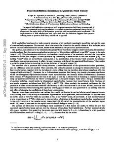
This integral diverges at k2 → ∞ as well as at k2 → 0. The former divergence is called ultraviolet divergence, the later is called infrared divergence. Any quantity, which is given by a divergent integral, is of course an ill-defined quantity. Therefore the first step is to make these integrals well-defined by introducing a regulator. There are several possibilities how this can be done, but the method of dimensional regularisation [1–3] has almost become a standard, as the calculations in this regularisation scheme turn out to be the simplest. Within dimensional regularisation one replaces the four-dimensional integral over the loop momentum by an D-dimensional integral, where D is now an additional parameter, which can be a non-integer or even a complex number. We consider the result of the integration as a function of D and we are interested in the behaviour of this function as D approaches 4. The original divergences will then show up as poles in the Laurent series in ε = (4 − D)/2. As a second example we consider a Feynman diagram contributing to the one-loop corrections for the process e+ e− → qgq, ¯ shown in fig. 1. At high energies we can ignore the masses of the electron and the light quarks. From the Feynman rules one obtains for this diagram (ignoring coupling and colour prefactors): µ
− v(p ¯ 4 )γ u(p5 )
1 p2123
Z
d D k1 1 p/12 k/1 k/3 u(p ¯ 1 )ε/(p2) 2 γν 2 γµ 2 γν v(p3 ). 4 2 (2π) k2 p12 k1 k3
(6)
Here, p12 = p1 + p2 , p123 = p1 + p2 + p3 , k2 = k1 − p12 , k3 = k2 − p3 . Further ε/(p2) = γτ ετ (p2 ), where ετ (p2 ) is the polarisation vector of the outgoing gluon. All external momenta are assumed 4
p5
p1 p2
p4
p3
Figure 1: A one-loop Feynman diagram contributing to the process e+ e− → qgq. ¯ to be massless: p2i = 0 for i = 1..5. We can reorganise this formula into a part, which depends on the loop integration and a part, which does not. The loop integral to be calculated reads: ρ
d D k1 k1 k3σ , (2π)4 k12 k22 k32
Z
(7)
while the remainder, which is independent of the loop integration is given by 1 − v(p ¯ 4 )γµ u(p5 ) 2 2 u(p ¯ 1 )ε/(p2)p/12 γν γρ γµ γσ γν v(p3 ). p123 p12
(8)
The loop integral in eq. (7) contains in the denominator three propagator factors and in the numerator two factors of the loop momentum. We call a loop integral, in which the loop momentum occurs also in the numerator a “tensor integral”. A loop integral, in which the numerator is independent of the loop momentum is called a “scalar integral”. The scalar integral associated to eq. (7) reads d D k1 1 . (2π)4 k12 k22 k32
Z
(9)
There is a general method [34, 35] which allows to reduce any tensor integral to a combination of scalar integrals at the expense of introducing higher powers of the propagators and shifted space-time dimensions. Therefore it is sufficient to focus on scalar integrals. Each integral can be specified by its topology, its value for the dimension D and a set of indices, denoting the powers of the propagators.
3 Multi-loop integrals Let us now consider a generic scalar l-loop integral IG in D = 2m − 2ε dimensions with n propagators, corresponding to a graph G. For each internal line j the corresponding propagator in the integrand can be raised to a power ν j . Therefore the integral will depend also on the numbers ν1 ,...,νn . It is sufficient to consider only the case, where all exponents are natural numbers: ν j ∈ N. We define the Feynman integral by n
∏ Γ(ν j )
IG =
j=1
Γ(ν − lD/2)
µ
� 2 ν−lD/2 5
Z
l
∏
r=1
d D kr iπ
D 2
n
1
∏ (−q2 + m2 )ν j , j=1
j
j
(10)
with ν = ν1 + ... + νn . µ is an arbitrary scale, called the renormalisation scale. The momenta q j of the propagators are linear combinations of the external momenta and the loop momenta. The prefactors are chosen such that after Feynman parametrisation the Feynman integral has a simple form: ! Z n n � U ν−(l+1)D/2 ν−lD/2 ν −1 . (11) IG = µ2 d n x δ(1 − ∑ xi ) ∏ x j j ν−lD/2 j=1
i=1
x j ≥0
F
The functions U and F depend on the Feynman parameters and can be derived from the topology of the corresponding Feynman graph G. Cutting l lines of a given connected l-loop graph such that it becomes a connected tree graph T defines a chord C (T, G) as being the set of lines not belonging to this tree. The Feynman parameters associated with each chord define a monomial of degree l. The set of all such trees (or 1-trees) is denoted by T 1 . The 1-trees T ∈ T 1 define U as being the sum over all monomials corresponding to the chords C (T, G). Cutting one more line of a 1-tree leads to two disconnected trees (T1 , T2 ), or a 2-tree. T 2 is the set of all such pairs. The corresponding chords define monomials of degree l + 1. Each 2-tree of a graph corresponds to a cut defined by cutting the lines which connected the two now disconnected trees in the original graph. The square of the sum of momenta through the cut lines of one of the two disconnected trees T1 or T2 defines a Lorentz invariant !2
∑
sT =
pj
.
(12)
j∈C (T,G)
The function F 0 is the sum over all such monomials times minus the corresponding invariant. The function F is then given by F 0 plus an additional piece involving the internal masses m j . In summary, the functions U and F are obtained from the graph as follows: i h U = ∑ ∏ xj , T ∈T 1 j∈C (T,G)
F0 =
∑
(T1 ,T2 )∈T 2
h
∏
j∈C (T1 ,G)
n
F
= F0 +U
i x j (−sT1 ) ,
∑ x j m2j .
(13)
j=1
4 Periods Periods are special numbers. Before we give the definition, let us start with some sets of numbers: The natural numbers N, the integer numbers Z, the rational numbers Q, the real numbers R and the complex numbers C are all well-known. More refined is already the set of algebraic ¯ An algebraic number is a solution of a polynomial equation with rational numbers, denoted by Q. coefficients: xn + an−1 xn−1 + · · · + a0 = 0, a j ∈ Q. 6
(14)
¯ is a sub-set of the complex numbers As all such solutions lie in C, the set of algebraic numbers Q ¯ are C. Numbers which are not algebraic are called transcendental. The sets N, Z, Q and Q countable, whereas the sets R, C and the set of transcendental numbers are uncountable. ¯ and C. There are several equivalent Periods are a countable set of numbers, lying between Q definitions for periods. Kontsevich and Zagier gave the following definition [36]: A period is a complex number whose real and imaginary parts are values of absolutely convergent integrals of rational functions with rational coefficients, over domains in Rn given by polynomial inequalities with rational coefficients. Domains defined by polynomial inequalities with rational coefficients are called semi-algebraic sets. We denote the set of periods by P. The algebraic numbers are contained in the set of periods: ¯ Q ∈ P. In addition, P contains transcendental numbers, an example for such a number is π: ZZ
π =
dx dy.
(15)
x2 +y2 ≤1
The integral on the r.h.s. clearly shows that π is a period. On the other hand, it is conjectured that the basis of the natural logarithm e and Euler’s constant γE are not periods. Although there are uncountably many numbers, which are not periods, only very recently an example for a number which is not a period has been found [37]. ¯ We need a few basic properties of periods: The set of periods P is a Q-algebra [36, 38]. In particular the sum and the product of two periods are again periods. The defining integrals of periods have integrands, which are rational functions with rational coefficients. For our purposes this is too restrictive, as we will encounter logarithms as integrands as well. However any logarithm of a rational function with rational coefficients can be written as ln g(x) =
Z1
dt
0
g(x) − 1 . (g(x) − 1)t + 1
(16)
5 A theorem on Feynman integrals Let us consider a general scalar multi-loop integral as in eq. (11). Let m be an integer and set D = 2m − 2ε. Then this integral has a Laurent series expansion in ε ∞
IG =
∑
c j ε j.
j=−2l
Theorem 1: In the case where 1. all kinematical invariants sT are zero or negative, 2. all masses mi and µ are zero or positive (µ 6= 0), 3. all ratios of invariants and masses are rational, 7
(17)
the coefficients c j of the Laurent expansion are periods. In the special case were 1. the graph has no external lines or all invariants sT are zero, 2. all internal masses m j are equal to µ, 3. all propagators occur with power 1, i.e. ν j = 1 for all j, the Feynman parameter integral reduces to IG =
Z
n
d n x δ(1 − ∑ xi ) U −D/2
(18)
i=1
x j ≥0
and only the polynomial U occurs in the integrand. In this case it has been shown by Belkale and Brosnan [39] that the coefficients of the Laurent expansion are periods. Using the method of sector decomposition we are able to prove the general case [40]. We will actually prove a stronger version of theorem 1. Consider the following integral ! Z n n r � �d +ε f ai +εbi n J = d x δ(1 − ∑ xi ) ∏ xi (19) ∏ Pj (x) j j . x j ≥0
i=1
i=1
j=1
The integration is over the standard simplex. The a’s, b’s, d’s and f ’s are integers. The P’s are polynomials in the variables x1 , ..., xn with rational coefficients. The polynomials are required to be non-zero inside the integration region, but may vanish on the boundaries of the integration region. To fix the sign, let us agree that all polynomials are positive inside the integration region. The integral J has a Laurent expansion ∞
J =
∑ c jε j.
(20)
j= j0
Theorem 2: The coefficients c j of the Laurent expansion of the integral J are periods. Theorem 1 follows then from theorem 2 as the special case ai = νi − 1, bi = 0, r = 2, P1 = U , P2 = F , d1 + ε f1 = ν − (l + 1)D/2 and d2 + ε f2 = lD/2 − ν. Proof of theorem 2: To prove the theorem we will give an algorithm which expresses each coefficient c j as a sum of absolutely convergent integrals over the unit hypercube with integrands, which are linear combinations of products of rational functions with logarithms of rational functions, all of them with rational coefficients. Let us denote this set of functions to which the integrands belong by M . The unit hypercube is clearly a semi-algebraic set. It is clear that absolutely convergent integrals over semi-algebraic sets with integrands from the set M are periods. In addition, the sum of periods is again a period. Therefore it is sufficient to express each coefficient c j as a finite sum of absolutely convergent integrals over the unit hypercube with integrands from M . To do so, we use iterated sector decomposition. This is a constructive method. Therefore we obtain as a side-effect a general purpose algorithm for the numerical evaluation of multi-loop integrals. 8
6 Sector decomposition In this section we review the algorithm for iterated sector decomposition [41–47]. The starting point is an integral of the form ! Z n r � n �λ µ (21) d n x δ(1 − ∑ xi ) ∏ xi i ∏ Pj (x) j , j=1
i=1
i=1
x j ≥0
where µi = ai + εbi and λ j = c j + εd j . The integration is over the standard simplex. The a’s, b’s, c’s and d’s are integers. The P’s are polynomials in the variables x1 , ..., xn . The polynomials are required to be non-zero inside the integration region, but may vanish on the boundaries of the integration region. The algorithm consists of the following steps: Step 0: Convert all polynomials to homogeneous polynomials. Step 1: Decompose the integral into n primary sectors. Step 2: Decompose the sectors iteratively into sub-sectors until each of the polynomials is of the form � mn ′ 1 P = xm (22) 1 ...xn c + P (x) ,
where c 6= 0 and P′ (x) is a polynomial in the variables x j without a constant term. In this case the mn 1 monomial prefactor xm 1 ...xn can be factored out and the remainder contains a non-zero constant term. To convert P into the form (22) one chooses a subset S = {α1 , ..., αk } ⊆ {1, ... n} according to a strategy discussed in the next section. One decomposes the k-dimensional hypercube into k sub-sectors according to Z1 0
n
d x =
1 k Z
∑
n
d x
k
∏
θ (xαl ≥ xαi ) .
(23)
i=1,i6=l
l=1 0
In the l-th sub-sector one makes for each element of S the substitution xαi = xαl x′αi for i 6= l.
(24)
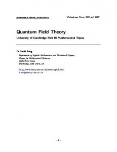
This procedure is iterated, until all polynomials are of the form (22). Fig. 2 illustrates this for the simple example S = {1, 2}. Eq. (23) gives the decomposition into the two sectors x1 > x2 and x2 > x1 . Eq. (24) transforms the triangles into squares. This transformation is one-to-one for all points except the origin. The origin is replaced by the line x1 = 0 in the first sector and by the line x2 = 0 in the second sector. Therefore the name “blow-up”. Step 3: The singular behaviour of the integral depends now only on the factor n
∏ xai i +εbi . i=1
9
(25)
x2
x2
6
x2
6
=
6
+
-
-
x1
-
x1 x′2
x1 x2
6
=
6
+ -
x1
-
x′1
Figure 2: Illustration of sector decomposition and blow-up for a simple example. We Taylor expand in the integration variables and perform the trivial integrations Z1
dx xa+bε =
0
1 , a + 1 + bε
(26)
leading to the explicit poles in 1/ε. Step 4: All remaining integrals are now by construction finite. We can now expand all expressions in a Laurent series in ε and truncate to the desired order. Step 5: It remains to compute the coefficients of the Laurent series. These coefficients contain finite integrals, which can be evaluated numerically by Monte Carlo integration. We implemented1 the algorithm into a computer program, which computes numerically the coefficients of the Laurent series of any multi-loop integral [45].
7 Hironaka’s polyhedra game In step 2 of the algorithm we have an iteration. It is important to show that this iteration terminates and does not lead to an infinite loop. There are strategies for choosing the sub-sectors, which guarantee termination. These strategies [48–52] are closely related to Hironaka’s polyhedra game. 1 The
program can be obtained from http://www.higgs.de/˜stefanw/software.html
10
x2
x2
6
x2
6
S={1,2},i=1
6
S={1,2},i=1
−→
−→
-
-
x1
x1
-
x1
Figure 3: Illustration of Hironaka’s polyhedra game. Hironaka’s polyhedra game is played by two players, A and B. They are given a finite set M of points m = (m1 , ..., mn ) in Nn+ , the first quadrant of Nn . We denote by ∆ ⊂ Rn+ the positive convex hull of the set M. It is given by the convex hull of the set [ � m + Rn+ . (27) m∈M
The two players compete in the following game: 1. Player A chooses a non-empty subset S ⊆ {1, ..., n}. 2. Player B chooses one element i out of this subset S. Then, according to the choices of the players, the components of all (m1 , ..., mn ) ∈ M are replaced by new points (m′1 , ..., m′n ), given by: m′j = m j , if j 6= i, m′i =
∑ m j − c,
(28)
j∈S
where for the moment we set c = 1. This defines the set M ′ . One then sets M = M ′ and goes back to step 1. Player A wins the game if, after a finite number of moves, the polyhedron ∆ is of the form ∆ = m + Rn+ ,
(29)
i.e. generated by one point. If this never occurs, player B has won. The challenge of the polyhedra game is to show that player A always has a winning strategy, no matter how player B chooses his moves. A simple illustration of Hironaka’s polyhedra game in two dimensions is given in fig. 3. Player A always chooses S = {1, 2}. In ref. [45] we have shown that a winning strategy for Hironaka’s polyhedra game translates directly into a strategy for choosing the sub-sectors which guarantees termination.
11
8 Shuffle algebras Before we continue the discussion of loop integrals, it is useful to discuss first shuffle algebras and generalisations thereof from an algebraic viewpoint. Consider a set of letters A. The set A is called the alphabet. A word is an ordered sequence of letters: w = l1 l2 ...lk .
(30)
The word of length zero is denoted by e. Let K be a field and consider the vector space of words over K. A shuffle algebra A on the vector space of words is defined by
∑
(l1 l2 ...lk ) · (lk+1 ...lr ) =
shuffles
σ
lσ(1) lσ(2) ...lσ(r),
(31)
where the sum runs over all permutations σ, which preserve the relative order of 1, 2, ..., k and of k + 1, ..., r. The name “shuffle algebra” is related to the analogy of shuffling cards: If a deck of cards is split into two parts and then shuffled, the relative order within the two individual parts is conserved. A shuffle algebra is also known under the name “mould symmetral” [53]. The empty word e is the unit in this algebra: e · w = w · e = w.
(32)
A recursive definition of the shuffle product is given by (l1 l2 ...lk ) · (lk+1 ...lr ) = l1 [(l2 ...lk ) · (lk+1 ...lr )] + lk+1 [(l1 l2 ...lk ) · (lk+2 ...lr )] .
(33)
It is well known fact that the shuffle algebra is actually a (non-cocommutative) Hopf algebra [54]. In this context let us briefly review the definitions of a coalgebra, a bialgebra and a Hopf algebra, which are closely related: First note that the unit in an algebra can be viewed as a map from K to A and that the multiplication can be viewed as a map from the tensor product A ⊗ A to A (e.g. one takes two elements from A, multiplies them and gets one element out). A coalgebra has instead of multiplication and unit the dual structures: a comultiplication ∆ and a counit e. ¯ The counit is a map from A to K, whereas comultiplication is a map from A to A ⊗ A. Note that comultiplication and counit go in the reverse direction compared to multiplication and unit. We will always assume that the comultiplication is coassociative. The general form of the coproduct is ∆(a) =
∑ ai
(1)
(2)
⊗ ai ,
(34)
i
(1)
(2)
where ai denotes an element of A appearing in the first slot of A ⊗ A and ai correspondingly denotes an element of A appearing in the second slot. Sweedler’s notation [55] consists in dropping the dummy index i and the summation symbol: ∆(a) = a(1) ⊗ a(2) 12
(35)
The sum is implicitly understood. This is similar to Einstein’s summation convention, except that the dummy summation index i is also dropped. The superscripts (1) and (2) indicate that a sum is involved. A bialgebra is an algebra and a coalgebra at the same time, such that the two structures are compatible with each other. Using Sweedler’s notation, the compatibility between the multiplication and comultiplication is expressed as � � � � (36) ∆ (a · b) = a(1) · b(1) ⊗ a(2) · b(2) . A Hopf algebra is a bialgebra with an additional map from A to A, called the antipode S , which fulfils � � � � (1) (1) (2) · a(2) = 0 for a 6= e. (37) =S a a ·S a
With this background at hand we can now state the coproduct, the counit and the antipode for the shuffle algebra: The counit e¯ is given by: e¯ (e) = 1,
e¯ (l1 l2 ...ln) = 0.
(38)
The coproduct ∆ is given by: k
∑
∆ (l1 l2 ...lk ) =
j=0
� � l j+1 ...lk ⊗ l1 ...l j .
(39)
The antipode S is given by:
S (l1 l2 ...lk ) = (−1)k lk lk−1 ...l2l1 .
(40)
The shuffle algebra is generated by the Lyndon words. If one introduces a lexicographic ordering on the letters of the alphabet A, a Lyndon word is defined by the property wi2 >...>ik >0 i1 xi11
(52)
The multiple polylogarithms are generalisations of the classical polylogarithms Lin (x), whose most prominent examples are ∞
Li1 (x) =
xi1 ∑ = − ln(1 − x), i1 =1 i1 15
∞
Li2 (x) =
xi1 ∑ 2, i1 =1 i1
(53)
as well as Nielsen’s generalised polylogarithms [63] Sn,p (x) = Lin+1,1,...,1 (x, 1, ..., 1), | {z }
(54)
Hm1 ,...,mk (x) = Lim1 ,...,mk (x, 1, ..., 1). | {z }
(55)
p−1
and the harmonic polylogarithms [64, 65]
k−1
In addition, multiple polylogarithms have an integral representation. To discuss the integral representation it is convenient to introduce for zk 6= 0 the following functions G(z1 , ..., zk; y) =
Zy 0
dt1 t1 − z1
Zt1 0
dt2 ... t2 − z2
tk−1 Z 0
dtk . tk − zk
(56)
In this definition one variable is redundant due to the following scaling relation: G(z1 , ..., zk; y) = G(xz1 , ..., xzk ; xy)
(57)
If one further defines g(z; y) =
1 , y−z
(58)
then one has d G(z1 , ..., zk ; y) = g(z1; y)G(z2 , ..., zk; y) dy
(59)
and G(z1, z2 , ..., zk ; y) =
Zy
dt g(z1 ;t)G(z2, ..., zk;t).
(60)
0
One can slightly enlarge the set and define G(0, ..., 0; y) with k zeros for z1 to zk to be G(0, ..., 0; y) =
1 (ln y)k . k!
(61)
This permits us to allow trailing zeros in the sequence (z1 , ..., zk ) by defining the function G with trailing zeros via (60) and (61). To relate the multiple polylogarithms to the functions G it is convenient to introduce the following short-hand notation: Gm1 ,...,mk (z1 , ..., zk; y) = G(0, ..., 0, z1 , ..., zk−1, 0..., 0, zk ; y) | {z } | {z } m1 −1
16
mk −1
(62)
Here, all z j for j = 1, ..., k are assumed to be non-zero. One then finds � � 1 1 1 k , , ..., ;1 . Lim1 ,...,mk (x1 , ..., xk ) = (−1) Gm1 ,...,mk x1 x1 x2 x1 ...xk
(63)
The inverse formula reads k
Gm1 ,...,mk (z1 , ..., zk; y) = (−1) Lim1 ,...,mk
�
� y z1 zk−1 , , ..., . z1 z2 zk
(64)
Eq. (63) together with (62) and (56) defines an integral representation for the multiple polylogarithms. Up to now we treated multiple polylogarithms from an algebraic point of view. Equally important are the analytical properties, which are needed for an efficient numerical evaluation. As an example I first discuss the numerical evaluation of the dilogarithm [66]: Li2 (x) = −
Zx
dt
0
∞ n ln(1 − t) x =∑ 2 t n=1 n
(65)
The power series expansion can be evaluated numerically, provided |x| < 1. Using the functional equations � � π2 1 1 − − (ln(−x))2 , Li2 (x) = −Li2 x 6 2 π2 (66) Li2 (x) = −Li2 (1 − x) + − ln(x) ln(1 − x). 6 any argument of the dilogarithm can be mapped into the region |x| ≤ 1 and −1 ≤ Re(x) ≤ 1/2. The numerical computation can be accelerated by using an expansion in [− ln(1 − x)] and the Bernoulli numbers Bi : ∞
Li2 (x) =
Bi
∑ (i + 1)! (− ln(1 − x))i+1 .
(67)
i=0
The generalisation to multiple polylogarithms proceeds along the same lines [67]: Using the integral representation eq. (56) one transforms all arguments into a region, where one has a converging power series expansion. In this region eq. (52) may be used. However it is advantageous to speed up the convergence of the power series expansion. This is done as follows: The multiple polylogarithms satisfy the Hölder convolution [58]. For z1 6= 1 and zw 6= 0 this identity reads G (z1 , ..., zw; 1) = � � � � w 1 1 j ∑ (−1) G 1 − z j , 1 − z j−1, ..., 1 − z1; 1 − p G z j+1, ..., zw; p . j=0
(68)
The Hölder convolution can be used to accelerate the convergence for the series representation of the multiple polylogarithms. 17
10 From Feynman integrals to multiple polylogarithms In sect. 3 we saw that the Feynman parameter integrals depend on two graph polynomials U and F , which are homogeneous functions of the Feynman parameters. In this section we will discuss how multiple polylogarithms arise in the calculation of Feynman parameter integrals. We will discuss two approaches. In the first approach one uses a Mellin-Barnes transformation and sums up residues. This leads to the sum representation of multiple polylogarithms. In the second approach one first derives a differential equation for the Feynman parameter integral, which is then solved by an ansatz in terms of the iterated integral representation of multiple polylogarithms. Let us start with the first approach. Assume for the moment that the two graph polynomials U and F are absent from the Feynman parameter integral. In this case we have n
Z1 0
n
ν −1
∏ dx j x j j j=1
!
∏ Γ(ν j )
n
δ(1 − ∑ xi ) = i=1
j=1
Γ(ν1 + ... + νn)
.
(69)
With the help of the Mellin-Barnes transformation we now reduce the general case to eq. (69). The Mellin-Barnes transformation reads −c
(A1 + A2 + ... + An )
1 1 = Γ(c) (2πi)n−1
Zi∞
dσ1 ...
Zi∞
dσn−1
(70)
−i∞
−i∞ σn−1 −σ1 −...−σn−1 −c . ×Γ(−σ1 )...Γ(−σn−1 )Γ(σ1 + ... + σn−1 + c) Aσ1 1 ...An−1 An
Each contour is such that the poles of Γ(−σ) are to the right and the poles of Γ(σ + c) are to the left. This transformation can be used to convert the sum of monomials of the polynomials U and F into a product, such that all Feynman parameter integrals are of the form of eq. (69). As this transformation converts sums into products it is the “inverse” of Feynman parametrisation. With the help of eq. (69) and eq. (70) we may exchange the Feynman parameter integrals against multiple contour integrals. A single contour integral is of the form 1 I = 2πi
γ+i∞ Z
dσ
γ−i∞
Γ(σ + a1 )...Γ(σ + am) Γ(−σ + b1 )...Γ(−σ + bn) −σ x . Γ(σ + c2 )...Γ(σ + c p) Γ(−σ + d1 )...Γ(−σ + dq)
(71)
If max (Re(−a1 ), ..., Re(−am )) < min (Re(b1 ), ..., Re(bn )) the contour can be chosen as a straight line parallel to the imaginary axis with max (Re(−a1 ), ..., Re(−am )) < Re γ < min (Re(b1 ), ..., Re(bn )) ,
(72)
otherwise the contour is indented, such that the residues of Γ(σ + a1 ), ..., Γ(σ + am ) are to the right of the contour, whereas the residues of Γ(−σ + b1 ), ..., Γ(−σ + bn ) are to the left of the contour. The integral eq. (71) is most conveniently evaluated with the help of the residuum 18
theorem by closing the contour to the left or to the right. To sum up all residues which lie inside the contour it is useful to know the residues of the Gamma function: res (Γ(σ + a), σ = −a − n) =
(−1)n , n!
res (Γ(−σ + a), σ = a + n) = −
(−1)n . n!
(73)
In general there are multiple contour integrals, and as a consequence one obtains multiple sums. Having collected all residues, one then expands the Gamma-functions: Γ(n + ε) = (74) � � Γ(1 + ε)Γ(n) 1 + εZ1 (n − 1) + ε2Z11 (n − 1) + ε3Z111 (n − 1) + ... + εn−1Z11...1 (n − 1) ,
where Zm1 ,...,mk (n) are Euler-Zagier sums defined by Zm1 ,...,mk (n) =
1
∑
n≥i1 >i2 >...>ik >0 i1
m1
...
1 i k mk
.
(75)
This motivates the following definition of a special form of nested sums, called Z-sums [68–71]: Z(n; m1 , ..., mk; x1 , ..., xk ) =
∑
xi11
n≥i1 >i2 >...>ik >0 i1
m1
...
xikk i k mk
.
(76)
k is called the depth of the Z-sum and w = m1 + ... + mk is called the weight. If the sums go to infinity (n = ∞) the Z-sums are multiple polylogarithms: Z(∞; m1 , ..., mk; x1 , ..., xk ) = Lim1 ,...,mk (x1 , ..., xk ).
(77)
For x1 = ... = xk = 1 the definition reduces to the Euler-Zagier sums [72–76]: Z(n; m1 , ..., mk; 1, ..., 1) = Zm1 ,...,mk (n).
(78)
For n = ∞ and x1 = ... = xk = 1 the sum is a multiple ζ-value [58, 77]: Z(∞; m1 , ..., mk; 1, ..., 1) = ζm1 ,...,mk .
(79)
The usefulness of the Z-sums lies in the fact, that they interpolate between multiple polylogarithms and Euler-Zagier sums. The Z-sums form a quasi-shuffle algebra. In this approach multiple polylogarithms appear through eq. (77). An alternative approach to the computation of Feynman parameter integrals is based on differential equations [65, 78–82]. To evaluate these integrals within this approach one first finds for each master integral a differential equation, which this master integral has to satisfy. The derivative is taken with respect to an external scale, or a ratio of two scales. An example for a
19
one-loop four-point function is given by p1
∂ ∂s123
p1
p2
p3
=
D−4 2(s12 + s23 − s123 )
p2
p3
1 2(D − 3) + (s123 − s12 )(s123 − s12 − s23 ) s123
p123
1 2(D − 3) + (s123 − s23 )(s123 − s12 − s23 ) s123
p123
1 − s12
1 − s23
p12
p23
.
The two-point functions on the r.h.s are simpler and can be considered to be known. This equation is solved iteratively by an ansatz for the solution as a Laurent expression in ε. Each term in this Laurent series is a sum of terms, consisting of basis functions times some unknown (and to be determined) coefficients. This ansatz is inserted into the differential equation and the unknown coefficients are determined order by order from the differential equation. The basis functions are taken as a subset of multiple polylogarithms. In this approach the iterated integral representation of multiple polylogarithms is the most convenient form. This is immediately clear from the simple formula for the derivative as in eq. (59).
11 Conclusions In this talk we reported on mathematical properties of Feynman integrals. We first showed that under rather weak assumptions all the coefficients of the Laurent expansion of a multi-loop integral are periods. In the second part we focused on multiple polylogarithms and how they appear in the calculation of Feynman integrals.
References [1] G. ’t Hooft and M. J. G. Veltman, Nucl. Phys. B44, 189 (1972). [2] C. G. Bollini and J. J. Giambiagi, Nuovo Cim. B12, 20 (1972). [3] G. M. Cicuta and E. Montaldi, Nuovo Cim. Lett. 4, 329 (1972). [4] S. Moch, J. A. M. Vermaseren, and A. Vogt, ph/0403192. 20
Nucl. Phys. B688, 101 (2004), hep-
[5] A. Vogt, S. Moch, and J. A. M. Vermaseren, ph/0404111.
Nucl. Phys. B691, 129 (2004), hep-
[6] L. W. Garland, T. Gehrmann, E. W. N. Glover, A. Koukoutsakis, and E. Remiddi, Nucl. Phys. B627, 107 (2002), hep-ph/0112081. [7] L. W. Garland, T. Gehrmann, E. W. N. Glover, A. Koukoutsakis, and E. Remiddi, Nucl. Phys. B642, 227 (2002), hep-ph/0206067. [8] S. Moch, P. Uwer, and S. Weinzierl, Phys. Rev. D66, 114001 (2002), hep-ph/0207043. [9] A. Gehrmann-De Ridder, T. Gehrmann, E. W. N. Glover, and G. Heinrich, Phys. Rev. Lett. 99, 132002 (2007), 0707.1285. [10] A. Gehrmann-De Ridder, T. Gehrmann, E. W. N. Glover, and G. Heinrich, JHEP 12, 094 (2007), 0711.4711. [11] A. Gehrmann-De Ridder, T. Gehrmann, E. W. N. Glover, and G. Heinrich, Phys. Rev. Lett. 100, 172001 (2008), 0802.0813. [12] A. Gehrmann-De Ridder, T. Gehrmann, E. W. N. Glover, and G. Heinrich, JHEP 05, 106 (2009), 0903.4658. [13] S. Weinzierl, Phys. Rev. Lett. 101, 162001 (2008), 0807.3241. [14] S. Weinzierl, JHEP 06, 041 (2009), 0904.1077. [15] S. Weinzierl, Phys. Rev. D80, 094018 (2009), 0909.5056. [16] S. Bloch, H. Esnault, and D. Kreimer, math.AG/0510011.
Comm. Math. Phys. 267, 181 (2006),
[17] S. Bloch and D. Kreimer, Commun. Num. Theor. Phys. 2, 637 (2008), 0804.4399. [18] S. Bloch, (2008), arXiv:0810.1313 [math.AG]. [19] F. Brown, Commun. Math. Phys. 287, 925 (2008), arXiv:0804.1660 [math.AG]. [20] F. Brown, (2009), arXiv:0910.0114 [math.AG]. [21] F. Brown and K. Yeats, (2009), arXiv:0910.5429 [math-ph]. [22] O. Schnetz, (2008), arXiv:0801.2856 [hep-th]. [23] O. Schnetz, (2009), arXiv:0909.0905 [math.CO]. [24] P. Aluffi and M. Marcolli, (2008), arXiv:0807.1690 [hep-th]. [25] P. Aluffi and M. Marcolli, (2008), arXiv:0811.2514 [hep-th]. 21
[26] P. Aluffi and M. Marcolli, (2009), arXiv:0901.2107 [math.AG]. [27] P. Aluffi and M. Marcolli, (2009), arXiv:0907.3225 [math-ph]. [28] C. Bergbauer, R. Brunetti, and D. Kreimer, (2009), arXiv:0908.0633 [hep-th]. [29] S. Laporta, Phys. Lett. B549, 115 (2002), hep-ph/0210336. [30] S. Laporta and E. Remiddi, Nucl. Phys. B704, 349 (2005), hep-ph/0406160. [31] S. Laporta, Int. J. Mod. Phys. A23, 5007 (2008), 0803.1007. [32] D. H. Bailey, J. M. Borwein, D. Broadhurst, and M. L. Glasser, (2008), arXiv:0801.0891 [hep-th]. [33] I. Bierenbaum and S. Weinzierl, Eur. Phys. J. C32, 67 (2003), hep-ph/0308311. [34] O. V. Tarasov, Phys. Rev. D54, 6479 (1996), hep-th/9606018. [35] O. V. Tarasov, Nucl. Phys. B502, 455 (1997), hep-ph/9703319. [36] M. Kontsevich and D. Zagier, in: B. Engquis and W. Schmid, editors, Mathematics unlimited - 2001 and beyond , 771 (2001). [37] M. Yoshinaga, (2008), arXiv:0805.0349 [math.AG]. [38] B. Friedrich, (2005), arXiv:math.AG/0506113. [39] P. Belkale and P. Brosnan, Int. Math. Res. Not. , 2655 (2003). [40] C. Bogner and S. Weinzierl, J. Math. Phys. 50, 042302 (2009), 0711.4863. [41] K. Hepp, Commun. Math. Phys. 2, 301 (1966). [42] M. Roth and A. Denner, Nucl. Phys. B479, 495 (1996), hep-ph/9605420. [43] T. Binoth and G. Heinrich, Nucl. Phys. B585, 741 (2000), hep-ph/0004013. [44] T. Binoth and G. Heinrich, Nucl. Phys. B680, 375 (2004), hep-ph/0305234. [45] C. Bogner and S. Weinzierl, Comput. Phys. Commun. 178, 596 (2008), 0709.4092. [46] A. V. Smirnov and M. N. Tentyukov, Comput. Phys. Commun. 180, 735 (2009), 0807.4129. [47] A. V. Smirnov and V. A. Smirnov, (2008), arXiv:0812.4700. [48] H. Hironaka, Ann. Math. 79, 109 (1964). [49] M. Spivakovsky, Progr. Math. 36, 419 (1983). [50] S. Encinas and H. Hauser, Comment. Math. Helv. 77, 821 (2002). 22
[51] H. Hauser, Bull. Amer. Math. Soc. 40, 323 (2003). [52] D. Zeillinger, Enseign. Math. 52, 143 (2006). [53] J. Ecalle, 23.html ).
(2002), (available at http://www.math.u-psud.fr/ biblio/ppo/2002/ppo2002-
[54] C. Reutenauer, Free Lie Algebras (Clarendon Press, Oxford, 1993). [55] M. Sweedler, Hopf Algebras (Benjamin, New York, 1969). [56] M. E. Hoffman, J. Algebraic Combin. 11, 49 (2000), math.QA/9907173. [57] L. Guo and W. Keigher, Adv. in Math. 150, 117 (2000), math.RA/0407155. [58] J. M. Borwein, D. M. Bradley, D. J. Broadhurst, and P. Lisonek, Trans. Amer. Math. Soc. 353:3, 907 (2001), math.CA/9910045. [59] A. B. Goncharov, Math. Res. Lett. 5, 497 (1998), (available at http://www.math.uiuc.edu/Ktheory/0297). [60] H. M. Minh, M. Petitot, and J. van der Hoeven, Discrete Math. 225:1-3, 217 (2000). [61] P. Cartier, Séminaire Bourbaki , 885 (2001). [62] G. Racinet, Publ. Math. Inst. Hautes Études Sci. 95, 185 (2002), math.QA/0202142. [63] N. Nielsen, Nova Acta Leopoldina (Halle) 90, 123 (1909). [64] E. Remiddi and J. A. M. Vermaseren, Int. J. Mod. Phys. A15, 725 (2000), hep-ph/9905237. [65] T. Gehrmann and E. Remiddi, Nucl. Phys. B601, 248 (2001), hep-ph/0008287. [66] G. ’t Hooft and M. J. G. Veltman, Nucl. Phys. B153, 365 (1979). [67] J. Vollinga and S. Weinzierl, Comput. Phys. Commun. 167, 177 (2005), hep-ph/0410259. [68] S. Moch, P. Uwer, and S. Weinzierl, J. Math. Phys. 43, 3363 (2002), hep-ph/0110083. [69] S. Weinzierl, Comput. Phys. Commun. 145, 357 (2002), math-ph/0201011. [70] S. Weinzierl, J. Math. Phys. 45, 2656 (2004), hep-ph/0402131. [71] S. Moch and P. Uwer, Comput. Phys. Commun. 174, 759 (2006), math-ph/0508008. [72] L. Euler, Novi Comm. Acad. Sci. Petropol. 20, 140 (1775). [73] D. Zagier, First European Congress of Mathematics, Vol. II, Birkhauser, Boston , 497 (1994).
23
[74] J. A. M. Vermaseren, Int. J. Mod. Phys. A14, 2037 (1999), hep-ph/9806280. [75] J. Blümlein and S. Kurth, Phys. Rev. D60, 014018 (1999), hep-ph/9810241. [76] J. Blümlein, Comput. Phys. Commun. 159, 19 (2004), hep-ph/0311046. [77] J. Blümlein, D. J. Broadhurst, and J. A. M. Vermaseren, (2009), arXiv:0907.2557 [mathph]. [78] A. V. Kotikov, Phys. Lett. B254, 158 (1991). [79] A. V. Kotikov, Phys. Lett. B267, 123 (1991). [80] E. Remiddi, Nuovo Cim. A110, 1435 (1997), hep-th/9711188. [81] T. Gehrmann and E. Remiddi, Nucl. Phys. B580, 485 (2000), hep-ph/9912329. [82] T. Gehrmann and E. Remiddi, Nucl. Phys. B601, 287 (2001), hep-ph/0101124.
24