May 11, 2010 - lation is given by the On-Shell recursion method of Britto, Cachazo, Feng and. Witten (BCFW) [44]. It turns out that for pure glue and gravity ...
University of California Los Angeles
Perturbative Quantum Gravity from Gauge Theory
A dissertation submitted in partial satisfaction of the requirements for the degree Doctor of Philosophy in Physics
by
John Joseph Carrasco
2010
c Copyright by ! John Joseph Carrasco 2010
To Elizabeth.
iii
Table of Contents
1 Introduction . . . . . . . . . . . . . . . . . . . . . . . . . . . . . . . .
3
1.1
Supergravity . . . . . . . . . . . . . . . . . . . . . . . . . . . . . .
5
1.2
Duality between Color and Kinematics . . . . . . . . . . . . . . .
7
2 Graphical techniques for scattering amplitudes . . . . . . . . . .
10
2.1
Outline of Unitarity Cut Evaluation . . . . . . . . . . . . . . . . .
12
2.2
4D Supersums in N = 4 super-Yang-Mills Theory . . . . . . . . .
16
2.2.1
MHV amplitudes . . . . . . . . . . . . . . . . . . . . . . .
16
2.2.2
The MHV Superspace . . . . . . . . . . . . . . . . . . . .
19
2.2.3
MHV superrules for non-MHV superamplitudes . . . . . .
22
2.2.4
Evaluation of N = 4 supersums in four dimensions . . . .
25
Graphical Terminology, Notation, and Conventions . . . . . . . .
26
2.3.1
Edges and Nodes . . . . . . . . . . . . . . . . . . . . . . .
26
2.3.2
Trees and Multi-Loop Graphs . . . . . . . . . . . . . . . .
27
2.3.3
Planar Graphs . . . . . . . . . . . . . . . . . . . . . . . .
28
2.3.4
Representations . . . . . . . . . . . . . . . . . . . . . . . .
29
2.3.5
Massless Amplitudes organized around Graphs . . . . . . .
30
Graphical Methods for Cut-Verification . . . . . . . . . . . . . . .
32
2.4.1
Identify Contributing Topologies . . . . . . . . . . . . . .
33
2.4.2
Topologies to Labelled Graphs . . . . . . . . . . . . . . . .
35
2.4.3
Sewing trees to multiloop graphs . . . . . . . . . . . . . .
36
2.3
2.4
iv
2.4.4
Dressing the Sewn Graphs . . . . . . . . . . . . . . . . . .
37
2.4.5
The question of Tree Dressing . . . . . . . . . . . . . . . .
39
2.4.6
Finding a set of spanning cuts. . . . . . . . . . . . . . . .
39
2.5
Cut-Construction . . . . . . . . . . . . . . . . . . . . . . . . . . .
41
2.6
Multiloop Gravity Amplitudes from tree-level KLT . . . . . . . .
44
3 The Ultraviolet Behavior of N = 8 Supergravity at Three Loops 45 4 The Ultraviolet Behavior of N = 8 Supergravity at Four Loops 54 5 Color-Kinematic Duality Generalization to Higher Loops . . .
62
6 Concluding Discussion . . . . . . . . . . . . . . . . . . . . . . . . .
70
References . . . . . . . . . . . . . . . . . . . . . . . . . . . . . . . . . . .
72
v
List of Figures
2.1
Graph representation of sample four-loop integrands. . . . . . . .
15
2.2
Examples of generalized four-loop cuts. . . . . . . . . . . . . . . .
15
2.3
MHV vertex construction. . . . . . . . . . . . . . . . . . . . . . .
22
2.4
Graph canonicalization towards evaluating planarity. . . . . . . .
28
2.5
Diagramatic representation of the ordered s-channel four-point tree graph. . . . . . . . . . . . . . . . . . . . . . . . . . . . . . . .
2.6
30
Graphs contributing to the four-point two-loop N = 4 yang-Mills amplitude. . . . . . . . . . . . . . . . . . . . . . . . . . . . . . . .
31
2.7
Three-particle two-loop planar cut. . . . . . . . . . . . . . . . . .
32
2.8
Diagramatic form of two loop four-point three-particle cut sewngraphs. . . . . . . . . . . . . . . . . . . . . . . . . . . . . . . . . .
3.1
Generalized cuts used to determine the three-loop four-point amplitude. . . . . . . . . . . . . . . . . . . . . . . . . . . . . . . . .
3.2
46
Loop integrals appearing in both N = 4 gauge-theory and N = 8 supergravity three-loop four-point amplitudes. . . . . . . . . . . .
3.3
39
48
The vacuum diagrams V (x) encoding the leading UV behavior of the individual N = 8 supergravity diagrams. . . . . . . . . . . . .
51
3.4
The ”no-triangle” multi-loop cut. . . . . . . . . . . . . . . . . . .
52
4.1
Four Loop vacuum graphs . . . . . . . . . . . . . . . . . . . . . .
55
4.2
Example graphs contributing to four loops. . . . . . . . . . . . . .
55
4.3
Four loop spanning cuts. . . . . . . . . . . . . . . . . . . . . . . .
57
vi
4.4
Example vacuum relations. . . . . . . . . . . . . . . . . . . . . . .
61
5.1
Example numerator identity. . . . . . . . . . . . . . . . . . . . . .
65
5.2
Diagrams contributing to three loops. . . . . . . . . . . . . . . . .
66
vii
List of Tables
3.1
Numerator factors of the four-point three-loop graphs for N = 4 super-Yang-Mills and N = 8 supergravity theories. . . . . . . . .
5.1
50
Numerator factors of the four-point three-loop graphs for the N = 4 super-Yang-Mills theory arranged to satisfy the loop level kinematiccolor duality.
. . . . . . . . . . . . . . . . . . . . . . . . . . . . .
viii
67
Acknowledgments My advisor, Professor Zvi Bern, is a world class scientist, teacher, mentor, and friend; I am profoundly grateful to have had these past five years. His leaps of understanding, generosity of spirit, passion, and patience will always amaze and inspire me. My closest collaborator and fellow Zvi-advisee, Henrik Johansson, was the perfect comrade for this adventure. I wish to thank him for his deep friendship, tireless conversation, eerily sharp insight, and fantastically opinionated stubbornness – all crucial for so much of the research presented here. I must thank Professors Lance Dixon, David Kosower, and Radu Roiban for their warm acceptance of Henrik and I into a collaboration responsible for much of the work directly relevant to this dissertation. I thank Tristen Dennen, Darren Forde, Harald Ita, and Yu-tin Huang for past and on-going collaborations directly related to this research. I have been fortunate enough to have met and been influenced by many people in the field over the past few years. Of direct relevance to the research presented here I wish to thank Nima Arkani-Hamed, Emil Bjerrum-Bohr, Henriette Elvang, Michael Kiermaier, Daniel Z. Freedman, Michael Green, Johannes Henn, David Skinner, Kelly Stelle, Pierre Vanhove and Christian Vergu for stimulating and provocative conversations, as well as encouragement. I thank the entire High Energy Theory group at UCLA for providing such an engaging environment. In a field where it is of course much easier to talk with one’s long-standing colleagues than jarring, eager, and largely unexposed minds, it is astounding to discover the pedagogical inclinations manifest in the Professors here at UCLA. I must first highlight Professor Eric D’Hoker who I have
ix
been fortunate enough to have for two formal courses: General Relativity, and a course on Lie Algebras1 . His warmth, and the care he puts into the coursework, is absolutely significant. I must also mention my gratitude for the courses taught by Professors Ernest Abers, Sergio Ferrara, Graciela Gelmini, Per Kraus, Alexander Kusenko, and Terry Tomboulis. To my regret, I have never had a formal course with Professor Michael Gutperle, but I am of course grateful for his friendliness and contributions to the string journal club. I cannot mention UCLA faculty and pedagogy without acknowledging my profound debt to Professor Robert Cousins who is directly responsible for my successful matriculation back into academia and, along with Professor Zvi Bern, the primary reason I applied to UCLA graduate school. I want to acknowledge the community of postdocs and fellow graduate students at UCLA. I particularly thank Joshua Davis, Warren Essey, John Estes, and Darya Krym for sharing their time, knowledge, friendship, and insights. I also especially thank Antoine Calvez, Marco Chiodaroli, Fernando Febres Cordero, Anthony Hall, James Hansen, Dammy Osoba, Kallia Petraki, Akhil Shah, and Ian Shoemaker for very enjoyable interactions. I, of course, thank Jenny Lee and Carol Finn for their tireless support of graduate students above and beyond the call of duty. I am deeply grateful for the financial support of the Gey Weyl Physics and Astronomy Alumni Fellowship, which in a very real sense is responsible for my level of productivity over the past three years. I would not be here were it not for my experiences as an undergraduate 1
I hope it does not escape the reader how relevant this subject matter is to the entire dissertation, but see esp. section 1.2.
x
at Caltech. Foremost I must thank my undergraduate advisor Professor John Preskill for his warmth, support, encouragement, and faith. My first exposure to Feynman’s path integral formalism for quantum mechanics was in a classical mechanics class taught by Professor Preskill, and my first course in quantum field theory was taught by his long-time friend Professor Mark Wise – I hope they are ok with what I’ve been doing with beautiful tools they handed me! I especially want to thank Professors Roger Blandford, Alan Weinstein, and Nai-Chang Yeh for their generous and passionate mentorship through Caltech’s wonderful Summer Undergraduate Research Fellowship program. These stronglypositive experiences at such a formative age were absolutely critical, not only for the important skills learned, but also for the requisite scientific confidence engendered. More personally, I thank Professors Nick Scoville and Tom Tombrello for their warmth and friendship very early on in my time at Caltech. I want to especially acknowledge the Caltech Associate Dean of Undergraduate Students, Barbara Greene for being wonderful. I want to close my academic acknowledgements by mentioning my debt to Dr. Kenneth Flurchick, my first physicist mentor, and a good friend, who introduced me to a) Mathematica, b) TEX, c) the satisfaction of simulation, and d) the realization that I wanted to be a physicist. I apologize for the laundry-list approach I now employ for more personal acknowledgements, but if I gave fair credit for how each has positively impacted my worldline it would out-mass my actual dissertation. For friendship, sanity, and inspiration I want to especially thank Nathan Bradshaw, Nate Bode, Vicki Brown, Drey Cameron, Frances Suyin Chance, Lily Chang, Meghann Chell, Connie Chang Chinchio, Richard Chino, Lucia Cordiero, Robert Cresswell, Jeremy
xi
Daw, Daniel Fain, Keri and Ben Franco, David Franey, Bridgid Fennell, Gary William Flake, Cem Yusef Gomel, Cecily Keim, David Liney, Richard Misenheimer, Anthony Frank Molinaro, Vanessa Morrison, Julie Park, Rebecca Peters, Anne Mariko Dudzik Pfarner, Connie and Ken Ramberg, Amanda Rounsaville, Paul Thomas Ryan, Marco Antonio Santos, Somayeh Shams, Steven Skovran, Tom Soulanille, Michelle Wilber, and Renee Medaglia Velez. Moreover, I am particularly indebted to lifelong friends Elizabeth Deneiges Carrasco, Noel John, Pat Helena, and Shain Vincent Murphy Carrasco, Ben Cerveny, Tod Edward Kurt, Michael Joseph Medaglia, Scott Charles Noble, and Preston Manly Pfarner for their insistence that I follow my dreams. I should point out that much of my personal philosophy of science was recently honed in 2004-2005 between Professor Christopher Hitchcock’s wonderful lectures, and night-long debates with Tod. I must also acknowledge that Tod pointed out, quite correctly and without even looking, which one of the (previously unpublished) diagrams in an earlier draft of this dissertation was completely wrong. Of course, Shain and I are who we are, and have accomplished what we have, ultimately because of our mother Pat, and our father Noel, who continue to guide, inspire, support, and challenge in exactly the right ways as they always have. Our entire family has supported our explorations, and I would especially like to thank our godparents Vincent Carrasco, Pamela Gallagher, Michael Murphy, and Maureen Ribeiro, and our grandparents Josephine and Vincent Carrasco, and Beatrice and John Joseph Murphy. I wish to thank my parents-in-law Robert Edward and Rose Marie Johnson for providing the world with Elizabeth, and for their warm support and encouragement of our adventures. I’m probably not the easiest son-in-law to have, but
xii
they’ve been wonderful. I would also like to acknowledge the love and friendship of my two sisters-in-law Kathleen Marie, and Jennifer Rebecca Johnson. Finally, none of this would have happened without the love, support, patience, beauty, inspiration, and friendship of my wife Elizabeth. Lest my prose veer uncontrollably to the potentially divergent ultraviolet, I will conclude by only remarking on and not describing the joy brought to me by our children Kathleen Solaar, who turned four in March, and Shain Tiberius, who turned two in April, and who are keeping their opinions as to the perturbative finiteness of N = 8 supergravity to themselves. Much of the work has already appeared in joint publications. Specifically the section on four-dimensional supersums in Chapter 2 is taken from [1], Chapter 3 is a version of [2], Chapter 4 is a version of [3], and Chapter 5 is a version of [4]. Additionally, material in Chapters 1 and 6 has appeared in [2], [3], and [4]. I should point out that important independent confirmations of the Yang-Mills amplitude used to construct the four-loop gravity result presented in Chapter 4 were generously performed by H. Elvang, and D. Freedman.
xiii
Vita
1975
Born, Maimonides Medical Center, Brooklyn, New York, USA
1993
Intern, North Carolina Supercomputing Center, Sponsor: Dr. Kenneth Flurchick.
1994
Caltech Summer Undergraduate Research Fellow, Sponsor: Professor Nai-Chang Yeh.
1995
Caltech Summer Undergraduate Research Fellow, Sponsor: Professor Roger Blandford.
1996
Caltech Summer Undergraduate Research Fellow, Sponsor: Professor Alan Weinstein.
1997
Developer, Jobtrak Corporation.
1998-2002
Engineer, Overture Services/GoTo.com.
2002-2004
Research Scientist, Overture Research/Yahoo! Labs.
2004
Caltech Summer Undergraduate Research Fellow, Sponsor: Professor John Preskill.
2005
B.S., Physics, California Institute of Technology
2005–2006
Teaching Assistant, Physics and Astronomy Department, University of California, Los Angeles.
2007–2010
Guy Weyl Physics and Astronomy Alumni Fellow.
xiv
Publications
Z. Bern, J. J. M. Carrasco and H. Johansson, “Perturbative Quantum Gravity from Gauge Theory,” arXiv: 1004.0476 [hep-th].
Z. Bern, J. J. M. Carrasco, L. J. Dixon, H. Johansson and R. Roiban, “The Ultraviolet Behavior of N = 8 Supergravity at Four Loops,” Phys. Rev. Lett. 103 081301, (2009). arXiv:0905.2326 [hep-th].
Z. Bern, J. J. M. Carrasco and H. Johansson, “Progress on Ultraviolet Finiteness of Supergravity,” arXiv:0902.3765 [hep-th].
Z. Bern, J. J. M. Carrasco, H. Ita, H. Johansson and R. Roiban, “On the Structure of Supersymmetric Sums in Multi-Loop Unitarity Cuts,” Phys. Rev. D 80 065029 (2009) arXiv: 0903.5348 [hep-th].
Z. Bern, J. J. M. Carrasco, L. J. Dixon, H. Johansson and R. Roiban, “Manifest Ultraviolet Behavior for the Three-Loop Four-Point Amplitude of N = 8 Supergravity,” Phys. Rev. D 78, 105019 (2008) [arXiv:0808.4112 [hep-th]].
Z. Bern, J. J. M. Carrasco and H. Johansson, “New Relations for Gauge-Theory Amplitudes,” Phys. Rev. D 78, 085011 (2008) [arXiv:0805.3993 [hep-ph]].
Z. Bern, J. J. Carrasco, D. Forde, H. Ita and H. Johansson, “Unexpected Cancellations in Gravity Theories,” Phys. Rev. D 77, 025010 (2008) [0707.1035 [hep-th]].
xv
Z. Bern, J. J. M. Carrasco, H. Johansson and D. A. Kosower, “Maximally supersymmetric planar Yang-Mills amplitudes at five loops,” Phys. Rev. D 76, 125020 (2007) [arXiv:0705.1864 [hep-th]].
Z. Bern, J. J. Carrasco, L. J. Dixon, H. Johansson, D. A. Kosower and R. Roiban, “Three-Loop Superfiniteness of N = 8 Supergravity,” Phys. Rev. Lett. 98, 161303 (2007) [arXiv:hep-th/0702112].
J. J. Carrasco, D. Fain, K. Lang, L. Zhukov. Clustering of bipartite advertiserkeyword graph, The ICDM 2003 Third IEEE International Conference on Data Mining, Workshop on Clustering Large Data Sets, Melbourne, Florida, 2003.
M. S. Yun, N. Z. Scoville, J. J. Carrasco, and R. D. Blandford. “Resolution and Kinematics of Molecular Gas Surrounding the Cloverleaf Quasar at z=2.6 Using the Gravitational Lens,” ApJ, 479 : L9-L13, 1997 April 10., [astro-ph/9702031].
xvi
Abstract of the Dissertation
Perturbative Quantum Gravity from Gauge Theory by
John Joseph Carrasco Doctor of Philosophy in Physics University of California, Los Angeles, 2010 Professor Zvi Bern, Chair
In this dissertation we present the graphical techniques recently developed in the construction of multi-loop scattering amplitudes using the method of generalized unitarity. We construct the three-loop and four-loop four-point amplitudes of N = 8 supergravity using these methods and the Kawaii, Lewellen and Tye treelevel relations which map tree-level gauge theory amplitudes to tree-level gravity theory amplitudes. We conclude by extending a tree-level duality between color and kinematics, generic to gauge theories, to a loop level conjecture, allowing the easy relation between loop-level gauge and gravity kinematics. We provide non-trivial evidence for this conjecture at three-loops in the particular case of maximal supersymmetry.
xvii
PREFACE “Keep an open mind, but not so open that your brains fall out.” - Multiple attributions. “... quantum field theory is the way it is because ... it is the only way to reconcile the principles of quantum mechanics ... with those of special relativity.” - S. Weinberg.[5] The last time I felt a need to struggle with the Heisenberg uncertainty principle for position and momentum my cognitive endpoint was “fine, complimentary basis, and so much for locality!” This is good – one should not fear representation theory especially not in the face of natural Fourier transforms. This same relation, applied to time and energy, still takes me to: “and so much for causality!”, even though the non-relativistic expression really refers to the characteristic time of an evolving system. My willingness to so readily extend locality discussions to causality illuminates an aspect of my thought-process that I enjoy, but can get me into trouble unchecked. Perhaps because of so many childhood hours spent programming rather than tinkering, my aesthetics are geared more towards consistency and clarity of description than checksumming against a collection of epistemological cornerstones. Clearly these are dangerous waters for an aspiring theorist. While experimentalists remain grounded through the collection of data, theorists have only calculation towards such data as pragmatic compass when at sea with potentially overly-flexible intuition. For this reason, primarily, as a graduate student I resolved to learn how to calculate to the best of my ability, in a realm still accessible to data2 . I refer to quantum field theoretic scattering amplitudes: the 2
Not, of course, in the maximally supersymmetric theories – but the same techniques apply to the more phenomenologically viable models.
1
gauge-invariant square root of cross-sections, the very quantity we measure when we bounce beams of particles off of each-other and collect statistics on the resulting end-states. I realize that much of the richness of quantum world we live in thrives in non-perturbative physics, not accessible even through the bound-state imaginary poles of the S-matrix. The discussion presented in this dissertation, however, involves only the banging of (massless) things together at energies dwarfing their interaction strength, seeing what comes out, and attempting to discern what truths may be evident. Finally, I should comment on my decision as a graduate student to focus on the scattering amplitudes of point-like quantum field theories–rather than those of extended structure frameworks like string theory. While one is certainly hard pressed to find modern physicists claiming that field-theory saturates the energetic bounds of current conceptualization, the framework of point-like field theory does seem to optimize the realm approached by both current experiment and computational ability. If Weinberg is correct, then any truths found here have to be valid limits of any more fundamental theoretic frameworks. If higher-genus string theory scattering amplitudes were easier to calculate then perhaps one would not find so useful the techniques presented in this dissertation, although structures like the discovered kinematic-color duality seem to be fairly universal. Similarly, had there been an explicit demonstration of four-dimensional divergence, higherloop calculations in the field theoretic limit of the maximally supersymmetric supergravity would be less well motivated. John Joseph M. Carrasco 11 May 2010 Los Angeles
2
CHAPTER 1 Introduction This dissertation engages the interface between gauge and gravity theories through the explicit calculation and understanding of scattering amplitudes. Although gauge and gravity theories have rather different physical behaviors they are intimately linked. The celebrated AdS/CFT correspondence [6] is the most striking such example, linking maximally supersymmetric gauge theory to supergravity in AdS space. Additionally, at weak coupling the tree-level (classical) scattering amplitudes of gauge and gravity theories are deeply intertwined because of the Kawai, Lewellen and Tye (KLT) relations [7]. These expressions, originally discovered in string theory, and first written down in the field theory limit over a decade ago, have implied a relation between tree-level gravity and gauge theories which has recently been clarified through the imposition of a tree-level duality between color-and-kinematics [8]. In quantum field theory, we describe classical scattering amplitudes using tree graphs: graphs without loops (cycles). For a fixed number of external particles, we associate increasingly quantum effects (scaling as increasing powers of Planck’s constant) with graphs containing larger numbers of loops. Physicists find multiloop calculations in gauge and gravity theories notoriously difficult when applying traditional methods. The difficulty arises because of an inherent combinatorial explosion in distinct graph topologies crossed with the sheer size of the analytic expressions associated with each graph. The fact that many of these graphs fail
3
to contribute, and that many of these expressions can be simplified to compact forms, suggests deep structure. Due to technical difficulties, until very recently, multi-loop calculations of gauge and gravity quantum field theories have proven very laborious when even possible. We have developed efficient and powerful techniques for constructing higherloop amplitudes in compact representations, based upon the generalized unitarity method. We present these techniques in Chapter 2. Applying this approach to calculations in gauge and gravity theories we find deep and, at times, unexpected structures [8, 1, 9], most easily seen in the most symmetric generalizations of these theories. While the explicit calculations presented in Chapters 3 and 4 are higher-loop four-particle interactions in maximally supersymmetric gauge and gravity theories, these techniques apply to lower-loop n-particle interactions in less symmetric theories, such as those needed to reduce the theoretical uncertainty obscuring upcoming LHC analysis. While the calculations presented here are driven primarily by questions regarding the ultraviolet behavior of N = 8 supergravity, recent years have seen a renaissance in the study of scattering amplitudes driven by the realization that they have far simpler and richer structures than visible from Feynman diagrams. Striking examples are the discoveries of twistor-space [10] and Grassmannian structures [11] in four dimensions for N = 4 super-Yang-Mills theory, as well as interpolations between weak and strong coupling [12, 13, 14]. In a rather distinct development, in the midst of our four-loop calculation in the maximally supersymmetric-Yang-Mills theory, we noted [8] that at tree level it was possible to impose a duality between color and kinematics for gauge theories, without altering the amplitudes. This has important consequences in clarifying the tree-level relation between gravity and gauge theory. As we shall argue in
4
Chapter 5, this duality also has the potential to greatly clarify the multi-loop structure of (super)gravity theories. We begin this introduction by reviewing the published arguments regarding the perturbative finiteness of the N = 8 supergravity theory, and conclude it by reviewing the tree-level kinematic-color duality for gauge theories and its implication for tree-level gravity amplitudes.
1.1
Supergravity
“Reports of the death of supergravity are exaggerations. One year everyone believed that supergravity was finite. The next year the fashion changed and everyone said that supergravity was bound to have divergences even though none had actually been found.” - S. Hawking.[15] While physicists do not know how to construct an ultraviolet-finite, pointlike quantum field theory of gravity in four dimensions, neither have they shown that such a construction is impossible. Point-like theories of gravity are nonrenormalizable because the gravitational coupling is dimensionful. To date, no known symmetry has proven capable of taming the divergences, leading to the widespread belief that all such theories require new physics in the ultraviolet (UV). These beliefs were historically an important motivation for the development of string theory. Were a finite four-dimensional point-like theory of gravity to be found, surely either a new symmetry or non-trivial dynamical mechanism must underpin it. The discovery of either would have a fundamental impact on our understanding of gravity. Supersymmetry has been studied extensively as a mechanism for taming UV divergences (see e.g. refs. [16, 17, 18]). Although assumptions about the existence of different types of superspaces lead to different power counting, any
5
superspace argument delays the onset of divergences only by a limited number of loops. For example, pure minimal (N = 1) supergravity cannot diverge until at least three loops [19, 20]. For maximal N = 8 supergravity [21], were a fully covariant superspace to exist, divergences would be delayed until seven loops. With the additional unconventional speculation that all fields respect tendimensional general coordinate invariance, one can even delay the divergence to nine loops [22]. Arguments [23] using the type II string non-renormalization theorems of Berkovits [24] suggest that divergences in the corresponding supergravity theory may indeed not arise before this loop order. However, in a recent paper the same authors have pointed out that technical issues starting at five loops invalidate this claim [25]. Instead, if no other mechanisms protect against ultraviolet divergences, a divergence would be expected to show up at seven loops in four dimensions, in agreement with the expectation from ref. [26]. Beyond this order, no known purely supersymmetric mechanism avoids divergences. String dualities also hint at additional cancellations in N = 8 supergravity [27], unless the situation is spoiled by towers of light nonperturbative states from branes wrapped on the compact dimensions [28]. Nonetheless, a different line of reasoning [29] using the unitarity method [30] has provided direct evidence that N = 8 supergravity may be UV finite to all loop orders. (See also ref. [31].) At one loop, all multi-graviton amplitudes in the theory can be expressed solely in terms of scalar box integrals; neither triangle nor bubble integrals appear [32, 33, 34]. Supersymmetry, factorization and infrared arguments provide strong evidence that the same is true for all one-loop amplitudes. This “no-triangle property” implies a set of surprising cancellations which go beyond any known supersymmetry argumentation. Generalized unitarity cuts, isolating one-loop subamplitudes inside higher-loop amplitudes, then imply specific multi-loop cancellations [29]. Are similar cancellations present in
6
all contributions to multi-loop amplitudes? Would they render the theory UV finite? In Chapters 3 and 4, we take concrete steps toward addressing these questions by calculating the complete three-loop and four-loop four-point amplitudes of N = 8 supergravity and analyzing their behavior. In Chapter 2 we establish the graphical methods necessary for their evaluation. In the next section we review a tree-level duality discovered in the process of calculating the four-loop four-point N = 8 supergravity amplitude, which in Chapter 5 we generalize to a loop-level conjecture which could prove very useful in higher-loop gravity exploration.
1.2
Duality between Color and Kinematics
To understand the relationship between tree-level gravity and gauge theory amplitudes, it is helpful to consider a gauge-theory amplitude where all particles are in the adjoint color representation. We can choose to write it in the following form, 1
g
Atree (1, 2, 3, . . . , n) = n−2 n
! ni ci " 2 , αi pαi i
(1.1)
where the sum runs over the (2n − 5)!! diagrams with only cubic vertices and the product runs over all propagators (internal legs) 1/p2αi of each diagram. The ci are √ the color factors obtained by dressing every three-vertex with an f#abc = i 2f abc structure constant, and the ni are kinematic numerator factors.
To satisfy the duality of [8], the diagrammatic numerators in eq. (1.1) should be arranged into a form that satisfies equations in one-to-one correspondence with the Jacobi identity of the color factors, ci = cj − ck ⇒ ni = nj − nk .
(1.2)
This duality is expected to hold in a large variety of theories, including super-
7
symmetric extensions of Yang-Mills theory. The ni are not gauge invariant but may be deformed under any shifts, ni → ni + ∆i , local or non-local, that satisfy the constraint, ! ∆i ci " 2 = 0. αi pαi i
(1.3)
We call this a generalized gauge transformation, as some of the invariance does not correspond to a gauge transformation in the traditional sense. An important subset of these transformations preserve the duality (1.2). This duality surprisingly implies new non-trivial relations between the color-ordered partial amplitudes of gauge theory [8]. An elegant proof of these relations has been made using monodromy for integrations in string theory [35]. Perhaps more striking is the observation [8] that once the gauge-theory amplitudes are arranged into a form satisfying the duality (1.2), gravity tree amplitudes are given by,
$ %(n−2) ! ni n 2 # " i2 , −i Mtree (1, 2, . . . , n) = n κ αi pαi i
(1.4)
where the n # represent numerator factors of a second gauge theory, the sum runs
over the same diagrams as in eq. (1.1), and κ is the gravitational coupling constant. This form of gravity tree amplitudes has been verified explicitly in field theory through eight points [8] using the KLT relations independent of whether or not the numerator factors are local (free of kinematic poles). If both families of kinematic factors are for N = 4 super-Yang-Mills theories, the gravity theory amplitudes are for N = 8 supergravity. If pure-Yang-Mills theory is instead used, the obtained gravity amplitudes correspond to Einstein gravity coupled to an anti-symmetric tensor and dilaton; the n-graviton treelevel amplitudes of this theory correspond to pure gravity. Additionally, the tilde numerator factors (˜ n) need not come from the same theory as the untilde factors.
8
This allows for the construction of gravity amplitudes with varying amounts of supersymmetry. These properties are now being understood in string theory [36, 37, 38]. The heterotic string, in particular, offers keen insight into these properties because of the parallel treatment of color and kinematics [37]. A field theory proof of eq. (1.4) has now been given [39] for an arbitrary number of external legs, assuming the duality (1.2) holds in a local form. We note that the invariance (1.3) implies that only one family of numerators (n or n #) needs to satisfy the duality (1.2), a
consequence independently realized by Kiermaier—see ref. [39] for more details. We also note that it is always possible to find a non-local duality- satisfying representation [40]. The open question at tree-level is whether or not it is always
possible to arrive at a local-form satisfying the duality. We will discuss the generalization to loop-level in Chapter 5.
9
CHAPTER 2 Graphical techniques for scattering amplitudes In this Chapter we present some of the graphical techniques recently developed in the construction of multi-loop scattering amplitudes using the method of generalized unitarity. There have been many recent advances in identifying the rich and clarifying structure underlying scattering amplitudes in many theories – not the least of which are maximally supersymmetric gauge and gravity theories [7, 10, 11, 12, 13, 14, 41]. These theories, because of their technical simplicity, have allowed the exploration of large multiplicity in addition to (relatively) high-loop order exploration. It is from these explorations that we first saw hints of the colorkinematic duality introduced at tree-level, and generalized to a loop-level property of gauge theories as described later in this dissertation. The natural representation for this duality, as well as recent higher-loop results, is an organization around trivalent momentum-flow graphs. Momentumflow graphs have the important property of topologically encoding the conservation of momenta. As we shall discuss, we can add structure to graphs to encode the order of edges around a vertex – convenient for consideration of color-order in the scattering amplitudes of gauge theories. The unitarity approach to multi-loop calculation uses knowledge of classical scattering amplitudes (tree-level) to construct quantum (loop-level) correc-
10
tions [30, 42, 43]. The primary method of tree-level scattering amplitude calculation is given by the On-Shell recursion method of Britto, Cachazo, Feng and Witten (BCFW) [44]. It turns out that for pure glue and gravity theories, and supersymmetric generalizations, only the three point (super)-amplitude must be specified – all others follow by recursion. We construct loop-level amplitudes by evaluating sufficient unitarity cuts to completely constrain the behavior of any given n-point loop level scattering amplitude. Detailed discussion of the evaluation of unitary cuts are given in the literature [30, 42, 43]. Especially noteworthy, for supersymmetric theories, are recent developments in the evaluation of supersums in 4 and 6 dimensions [1, 45, 46]. Tacitly involved in the application of the unitarity method, but having received less attention in the literature, are the required graphical techniques for the building and organizing of results. This is largely because, until fairly recently, the number of relevant contributing topologies had been fairly light. In particular, the four-point two-loop scattering amplitude for maximally supersymmetric supergravity requires only two graphs [47]. For four-point three-loop, as discussed in Chapter 3 we require only nine graphs. The graphical techniques for the construction and verification of these amplitudes is readily accomplished by hand1 using intuition built up from Feynman graph calculation. But for the full four-point four-loop amplitude, even for maximally symmetric super-Yang-Mills theory, we have 50 topologies contributing, and thousands of cuts to preform. We therefore find it convenient to formalize our techniques for graphical calculation towards automation, and present the results of that effort here. We will open this Chapter with a brief review of the unitary method in section 2.1. Following that, in section 2.2 we will review a simple algorithim for 1
With the exception of the four-particle cuts of three-loops, which initiated the development of many of the techniques described in this dissertation.
11
performing supersums in maximally supersymmetric N = 4 super-Yang-Mills theory. In section 2.4 we discuss graphical methods as applied to cut-verification – the problem of confirming that a given expression for a scattering amplitude satisfies all relevant cuts. In section 2.5 we will discuss how these same graphical methods can be used for constructing multi-loop amplitudes. We conclude in section 2.6 with a brief remark on how graphical organization can be used through the tree-level KLT relations to build loop-level gravity scattering amplitudes.
2.1
Outline of Unitarity Cut Evaluation
This section outlines the general approach to unitary cut-evaluation. This is how we extract data relevant to particular theories. Once we have this data we can begin to organize it in terms of graphs as discussed in section 2.5. The unitarity method systematically constructs multi-loop amplitudes from lower-loop amplitudes. The widest applicability so far has mostly been in massless theories – although in principle it generalizes to massive theories as well. The primary technical advantage of the approach is that for each stage of the calculation one need only consider on-shell expressions. For both gauge and gravity amplitudes this amounts to a simplification that avoids consideration of gauge-fixing, ghosts, etc, in favor of completely gauge-independent expressions. This method and various refinements have been described in some detail in various references [9, 30, 47, 48, 49], so in this section we only offer a brief review of four-dimensional techniques, and references to more thorough discussions. While the technical advantages of the unitarity method is what is largely lauded, we feel that it is important to recognize that the implicit organization has always been in terms of theory-independent momentum-flow graphs. Momentum flow graphs
12
make manifest the conservation of momenta – a very physical symmetry – and allow, via modest extension, for a manifest representation of the necessary colorordering for gauge theory amplitudes. This made it the natural representation to discover the kinematic-color discussed already at tree-level, and later generalized to loop corrections, in this dissertation. The procedure of checking that a graphically organized expression satisfies a cut we will call cut-verification and the steps associated with the graphical part of cut-verification will be discussed in section 2.4. The part of cut-verification that is explicitly concerned with the evaluation of the sum over products of lower-level amplitudes we will call cut-evaluation. Cut-evaluation requires only the ability to sum the product of contributing amplitudes over the states of the theory. When considering a particular cut of a multi-loop amplitude down to tree-level, cut evaluation is simply evaluating: !
states
tree tree tree Atree (1) A(2) A(3) · · · A(m) ,
(2.1)
using kinematics that place all cut legs on-shell, li2 = 0. While straightforward conceptually, expressions for D-dimensional amplitudes can be unwieldy, and naive brute-force component consideration of every state crossing the cuts can prove messy. Superspace methods in four [45] and recently six dimensions [46] have been developed which alleviate much of the complexity. While a thorough discussion would distract unduly from a Chapter focussed on graphical methods, to convey the simplicity, in the following section we will quote a simple algorithm [1] for calculating the supersums of N = 4 super-Yang-Mills amplitudes. The actual building of a multi-loop amplitude we will call cut-construction and it amounts to constraining ansatze for an amplitude under a spanning set of cut-verifications. The ansatze we discuss here will be organized around tri-valent momentum flow graph topologies. We will assume that every topology will con-
13
tribute to the amplitude expression via integrand denominators D(graphi ) equal to the product of the Lorentz square of the momentum of flowing along every internal edge. Also, depending upon the theory, each graph will contribute expressions in terms of a kinematic numerator associated with the topology, an appropriate integration measure for loop integrals, and graph-dependent colorfactors for gauge theory amplitudes. The a priori construction of such ansatze is simplest for maximally supersymmetric four-point amplitudes where symmetry arguments imply that the ratio between the loop integrand and the tree amplitudes is a rational function solely of Lorentz dot products. For higher-point amplitudes similar ratios necessarily contain either spinor products or other (e.g. Levi-Civita) tensors. The method of maximal cuts, discussed in some detail in section 2.5, allows for the systematic construction of the ansatz by considering a particular set of cuts in a particular order. In fig. 2.2, we display a few unitarity cuts that have to be analyzed at three and four loops. If no solution to all cut conditions is found, then it is necessary enlarge the ansatz until one is found. As will be discussed in section 2.4.6, at the heart of the unitarity method is the realization that the expression for any multi-loop amplitude must satisfy every relevant cut, even down to tree level. A spanning set of cuts will ensure that an expression has all the correct off-shell information in every physical channel. A potential theory-dependent concern, when only working in four-dimensions, is that cut-construction may miss rational-pieces. Fortunately, rational-pieces are cut-contributing in D-dimensions under dimensional regularization. The terms obtained from a single cut are generally ambiguous, since the numerator may be freely modified by adding terms which vanish on the cut in question, e.g. those terms proportional to "2i where "i are momenta of cut lines.
14
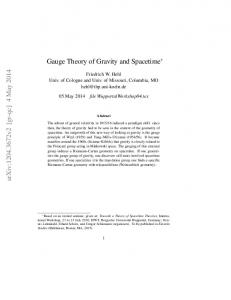
After considering a complete set of cuts –the only remaining ambiguities are terms which are free of cuts in every channel. In D-dimensions these ambiguities always sum to zero in the full amplitude. For simple cuts, the sum over states in eq. (2.1), can be easily evaluated in components, making use of supersymmetry Ward identities [50], as discussed for the three-particle cut of the two loop four-point amplitude presented in ref. [47]. However, for more general situations, we need a convenient means for evaluating the sums over supersymmetric amplitudes. In the following section we present an algorithm for N = 4 super-Yang-Mills theory.
Figure 2.1: Graph representation of sample integrands appearing in the final result for the four-loop amplitudes. The first two integrands are planar and the last one is nonplanar. Every edge in this figure is an off-shell Feynman propagator. These integrands have kinematic numerators which can be determined in any given theory by comparing the cuts of an ansatz for the numerator against the cuts of the amplitude.
Figure 2.2: Some examples of generalized cuts at four loops. Every exposed line is cut and satisfies on-shell conditions. Diagrams (b) and (c) are near maximal cuts.
15
2.2
4D Supersums in N = 4 super-Yang-Mills Theory
While a thorough discussion on superpsace and supersums would distract unduly from a Chapter focused on graphical methods, in this section we will quote a simple algorithm for calculating the supersums of N = 4 super-Yang-Mills amplitudes in external gluons. Towards this end we must first review some fourdimensional formalism. This review and the presented algorithm closely follow ref. [1]. This discussion is of necessity fairly technical. It can be safely skipped if the reader is mostly interested in graphical methods.
2.2.1
MHV amplitudes
The vector multiplet of the N = 4 supersymmetry algebra consists of one gluon, four gluinos and three complex scalars, all in the adjoint representation of the gauge group, which here we take to be SU(Nc ). With all states in the adjoint representation, any complete tree-level amplitude can be decomposed as n−2 Atree n (1, 2, 3, . . . , n) = g
!
P(2,3,...,n)
Tr[T a1 T a2 T a3 · · · T an ] Atree n (1, 2, 3, . . . , n), (2.2)
where Atree are tree-level color-ordered n-leg partial amplitudes. The T ai ’s are n generators of the gauge group and encode the color of each external leg 1, 2, 3 . . . n, with color group indices ai . The sum runs over all noncyclic permutations of legs, which is equivalent to all permutations keeping one leg fixed (here leg 1). Helicities and polarizations are suppressed. We use the all outgoing convention for the momenta to define the amplitudes. All states transform in antisymmetric tensor representations of the SU(4) R-symmetry group such that states with opposite helicities are in conjugate representations. The R-symmetry and helicity quantum numbers uniquely specify
16
all on-shell states: g+ ,
f+a ,
sab ,
f−abc ,
abcd g− ,
(2.3)
where g± and f± are, respectively, the positive and negative helicity gluons and gluinos while sab are scalars. (The scalars are complex-valued and obey a selfduality condition which will not be relevant here.) These fields are completely antisymmetric in their displayed R-symmetry indices—denoted by a, b, c, d—which transform in the fundamental representation of SU(4), giving a total of 16 states in the on-shell multiplet. Alternatively, we can use the dual assignment obtained by lowering the indices with a properly normalized Levi-Civita symbol εabcd , giving the fields, + gabcd ,
+ fabc ,
sab ,
fa− ,
g− .
(2.4)
We will use both representations to describe the amplitudes of N = 4 superYang-Mills theory. For MHV amplitudes we will mainly use the states with upper indices in eq. (2.3) whereas for MHV we will use mainly the states with lower indices in eq. (2.4). This is a matter of convenience, and the two sets of states may be interchanged, as we will briefly discuss later in this section. We begin by discussing the MHV amplitudes, which we define as an amplitude with a total of eight (2 × 4 distinct) upper SU(4) indices. (In order to respect SU(4) invariance, amplitudes of the fields in eq. (2.3) must always come with 4m distinct upper indices, where m is an integer. Furthermore amplitudes with four or zero indices vanish as they are related by supersymmetry to vanishing [50]
17
amplitudes.) Some simple examples of MHV amplitudes are, '1 2(4 (a) : =i , '1 2( '2 3( '3 4( '4 1( '1 2(3 '1 3( − − + + (b) : Atree (1 , 2 , 3 , 4 ) = i , 4 g g abcd f abc fd '1 2( '2 3( '3 4( '4 1( '1 2(2 '1 3( '2 3( tree − − + (c) : A4 (1f abc , 2f abd , 3scd , 4g ) = i , '1 2( '2 3( '3 4( '4 1( − − + + Atree 4 (1g abcd , 2g abcd , 3g , 4g )
(2.5)
where a, b, c, d are four distinct fundamental SU(4) indices. The overall phases of these amplitudes depend on conventions. We will fix this ambiguity by demanding that the phases be consistent with the supersymmetry algebra, which is automatically enforced when using superspace. The amplitudes are written in terms of the familiar holomorphic and antiholomorphic spinor products, 'i j( = 'i|j( = u¯− (pi )u+ (pj ) = εαβ λαi λβj , ˙
˜ α˙ λ ˜β [i j] = [i|j] = u¯+ (pi )u− (pj ) = εα˙ β˙ λ i j ,
(2.6)
˜ α˙ are commuting spinors which may be identified with the where the λαi and λ i positive and negative chirality solutions |i( = u+ (pi ) and |i] = u− (pi ) of the massless Dirac equation and the spinor indices are implicitly summed over. These products are antisymmetric, 'i j( = − 'j i(, [i j] = − [j i]. Momenta are related to these spinors via ˜ α˙ pµi σµαα˙ = λαi λ i
or
pµi σµ = |i([i| ,
(2.7)
and similar formulæ hold for the expression of pµi σ µ . We often write simply pi = |i([i| or sometimes p = |p([p|. The proper contractions of momenta pi with spinorial objects will be implicitly assumed below. Typically, we will denote external momenta by ki and loop momenta by li . A subtlety we must deal with is a slight inconsistency in the standard spinor helicity formalism for massless particles when a state crosses a cut. In a given cut
18
we will always have the situation that on one side of a cut line the momentum is outgoing, but on the other side it is incoming. Thus across a cut we encounter expressions such as |−i([i|, which is not properly defined in our all-outgoing conventions and can lead to incorrect phases. This is because the spinor |−i( carries momentum −pi , and thus it has an energy component of opposite sign to that carried by the spinor [i|. This problem is due to the fact that the spinor helicity formalism does not distinguish between particle and antiparticle spinors, as has been discussed and corrected in refs. [51] for the MHV vertex expansion, and for BCFW recursion relations with fermions. To deal with this, we use the analytic continuation rule that the change of of sign of the momentum is realized by the change in sign of the holomorphic spinor [52], pi )→ −pi
2.2.2
↔
λαi )→ −λαi ,
↔
| − i( )→ −|i( ,
˜ α˙ )→ λ ˜ α˙ , λ i i | − i] )→ |i] .
(2.8)
The MHV Superspace
The supersymmetry relations between the different MHV amplitudes may be encoded in an on-shell superspace, which conveniently packages all amplitudes into a single object—the generating function or superamplitude. Each term in the superamplitude corresponds to a regular component scattering amplitude. Depending upon the detailed formulation of the superspace, scattering amplitudes of gluons, fermions and scalars are then formally extracted either by the application of Grassmann-valued derivatives [52], or, equivalently, by multiplying with the appropriate wave functions and integrating over all Grassmann variables [53, 10]. Effectively, these operations amount to selecting the component amplitude with the desired external states.
19
The MHV generating function (or superamplitude) is defined as, &! ' i (8) α a δ λj ηj , j=1 'j (j + 1)( j=1 n
AMHV (1, 2, . . . , n) n
≡ "n
(2.9)
where the leg label n+1 is identified with the leg label 1, and ηja are 4n Grassmann odd variables labeled by leg j and SU(4) R-symmetry index a. As indicated by the cyclic denominator, this amplitude is color ordered (i.e., it is the kinematic coefficient of a particular color trace in eq. (2.2)), even though the numerator possesses full crossing symmetry having encoded all possible MHV helicity and ( particle assignments. We suppress the delta-function factor (2π)4 δ (4) ( i pi ) = ( ˜ (2π)4 δ (4) ( i λi λ i ) responsible for enforcing the overall momentum conservation. The eightfold Grassmann delta function in (2.9) is a product of pairs of delta
functions, each pair being associated with one of the possible values of the SU(4) R-symmetry index: δ (8)
n &! i=1
4 n &! ' ) ' λαi ηia = δ (2) λαi ηia . a=1
(2.10)
i=1
This expression can be further expanded, δ
(8)
n &!
λαi ηia
i=1
'
=
4 ! n ) a=1 i 1) .
(3.2)
The bound (3.2) differs somewhat from earlier superspace power counting [63],
45
Figure 3.1: Generalized cuts used to determine the three-loop four-point amplitude. although all bounds confirm UV finiteness of N = 4 super-Yang-Mills theory in D = 4. The bound (3.2) has been proven to all orders [18] using N = 3 harmonic superspace [64]. Explicit computations show that it is saturated through four loops [62, 47, 65, 29]. The N = 8 supergravity bound (3.1) corresponds, in the language of effective actions, to a one-particle irreducible effective action starting with loop integrals multiplied by D 4 R4 at each loop order beyond L = 1. Here R4 is a shorthand for the supersymmetrization of a particular contraction of four Riemann tensors [20], and D denotes a generic covariant derivative. The stronger, “superfinite” bound (3.2), if applied to N = 8 supergravity, would differ from eq. (3.1) beginning at L = 3 for general D, although both bounds imply three-loop finiteness for D = 4. It corresponds to a three-loop effective action beginning with D 6 R4 , not D 4 R4 . As the supergravity finiteness bound (3.1) is based on only a limited set of unitarity cuts [47], additional (stronger) cancellations may be missed [29]. To study this issue, we use the unitarity method [30, 62] to build the threeloop four-point N = 8 supergravity amplitude. In this method, on-shell tree amplitudes suffice as ingredients for computing amplitudes at any loop order. The reduction to tree amplitudes is crucial. It allows the use of the KawaiLewellen-Tye (KLT) [7] tree-level relations between gravity and gauge theory amplitudes [47], effectively reducing gravity computations to gauge theory ones.
46
The original KLT relations express tree-level closed-string scattering amplitudes in terms of pairs of open-string ones. The perturbative massless states of the closed and open type II superstring compactified to four dimensions on a torus, are those of N = 8 supergravity and N = 4 super-Yang-Mills theory, respectively. Thus, in the limit of energies well below the string scale, the KLT relations express N = 8 supergravity tree amplitudes as quadratic combinations of N = 4 superYang-Mills tree amplitudes (see e.g. ref. [32]). At tree level there are no subtleties in taking this limit. We use the generalized unitarity cuts [42] illustrated in fig. 3.1. Together with the iterated two-particle cuts evaluated in refs. [62, 47], these cuts completely determine any massless three-loop four-point amplitude. Since we are interested in the UV behavior of the amplitudes in D dimensions, the unitarity cuts must be evaluated in D dimensions [43]. This renders the calculation more difficult, because powerful four-dimensional spinor methods cannot be used. Some of the D-dimensional complexity is avoided by performing internal-state sums in terms of the simpler on-shell gauge supermultiplet of D = 10, N = 1 super-Yang-Mills theory instead of the D = 4, N = 4 multiplet. We have also performed various four-dimensional cuts, which in practice provide a very useful guide. Our computation proceeds in two stages. In the first stage we deduce the three-loop N = 4 super-Yang-Mills amplitudes from generalized cuts, including cuts (a)-(c) in fig. 3.1, and the iterated two-particle cuts analyzed in refs. [62, 47]. From the cuts we obtain a loop-integral representation of the amplitude. The diagrams in fig. 3.2 describe the scalar propagators for the loop integrals. The numerator factor for each integral in the super-Yang-Mills case is given in the second column of table 3.1. In the second stage we use the KLT relations to write the cuts of the N = 8
47
2
3
2
3
2
3
1
4
1
4
1
4
2
3
1
4
2
3
2
3
1
4
1
4
2
3
2
3
2
3
1
4
1
4
1
4
Figure 3.2: Loop integrals appearing in both N = 4 gauge-theory and N = 8 supergravity three-loop four-point amplitudes. The integrals are specified by combining the diagrams’ propagators with numerator factors given in table 3.1. supergravity amplitude as sums over products of pairs of cuts of the corresponding N = 4 super-Yang-Mills amplitude, including twisted non-planar contributions. The iterated two-particle cuts studied in ref. [47], together with the cuts in fig. 3.1 evaluated here, suffice to fully reconstruct the supergravity amplitude. We find that the three-loop four-point N = 8 supergravity amplitude in D dimensions is, (3)
M4
=
& κ '8 !, I (a) + I (b) + 21 I (c) + 14 I (d) stuM4tree 2 S3 + 2I (e) + 2I (f) + 4I (g) + 12 I (h) + 2I (i) ,
(3.3)
where S3 represents the six independent permutations of legs {1, 2, 3}, κ is the gravitational coupling, and M4tree is the supergravity four-point tree amplitude. The I (x) (s, t) are D-dimensional loop integrals corresponding to the nine diagrams
48
in fig. 3.2, with numerator factors given in the third column of table 3.1. The Mandelstam invariants are s = (k1 + k2 )2 , t = (k2 + k3 )2 , u = (k1 + k3 )2 . The numerical coefficients in front of each integral in eq. (3.3) are symmetry factors of the diagrams. Remarkably, the number of dimensions appears explicitly only in the loop integration measure. We remark that the amplitude (3.3) could be used to study D = 11, N = 1 supergravity compactified on a circle or two-torus at three loops, just as the two-loop amplitude [47] was analyzed in ref. [66]. That analysis, along with the assumption that M-theory dualities hold at this loop order, restricts the type II string effective action at three loops to start with D 6 R4 , not D 4 R4 . With the explicit expression for the amplitude (3.3) in hand, we may determine the UV behavior straightforwardly. In the super-Yang-Mills case, the entries in the second column in table 3.1 contain no more than two powers of loop momenta. Accounting for the ten propagators of each diagram in fig. 3.2 and the three-loop integration measure, we see that each integral separately satisfies the known super-Yang-Mills finiteness bound (3.2). In contrast, the supergravity numerators, as given in the third column of table 3.1, contain up to four powers of loop momenta. Separately, these integrals satisfy the bound (3.1). The iterated two-particle cuts evaluated in ref. [47] give the integrals (a)-(g) in fig. 3.2 and table 3.1. All such contributions have numerator factors which are squares of the Yang-Mills ones. The entries (h) and (i) are new and do not have this structure. Might there be additional cancellations between the integrals in the N = 8 supergravity case? To check this, we expand each integral in a series in the external momenta, keeping only the leading terms. We thereby keep terms with maximal powers of loop momenta and set the external momenta to zero in the
49
Table 3.1: The numerator factors of the integrals I (x) in fig. 3.2. The first column labels the integral, the second column the relative numerator factor for N = 4 super-Yang-Mills, the third column the factor for N = 8 supergravity. In the Yang-Mills case an overall factor of stAtree has been removed, while in the super4 gravity case an overall factor of stuM4tree has been removed. The loop momenta 2 li are the momenta of the labeled propagators in fig. 3.2, and li,j = (li + lj )2 .
Integral I (x)
N = 4 Super-Yang-Mills
N = 8 Supergravity
(a)–(d)
s2
[s2 ]2
(e)–(g)
s(l1 + k4 )2
[s (l1 + k4 )2 ]2
(h)
2 2 sl1,2 + tl3,4 − sl52 − tl62 − st
2 2 (sl1,2 + tl3,4 − st)2 2 − s2 (2(l1,2 − t) + l52 )l52 2 − t2 (2(l3,4 − s) + l62 )l62
− s2 (2l12 l82 + 2l22 l72 + l12 l72 + l22 l82 ) 2 2 − t2 (2l32 l10 + 2l42 l92 + l32 l92 + l42 l10 )
+ 2stl52 l62 (i)
2 2 sl1,2 − tl3,4 − 31 (s − t)l52
2 2 2 (sl1,2 − tl3,4 ) 2 2 − (s2 l1,2 + t2 l3,4 + 31 stu)l52
50
Figure 3.3: The vacuum diagrams V (x) encoding the leading UV behavior of the individual N = 8 supergravity diagrams. Dots on propagators represent squared propagators. The shaded cross in diagram (c) represents a numerator factor of l2 , where l is the momentum of a collapsed vertical propagator. propagators. Each integral reduces to a sum of vacuum diagrams, possibly with squared propagators. Fig. 3.3 shows the resulting vacuum diagrams V (x) . Integrals (a)-(d) in fig. 3.2 have no powers of loop momenta in their numerators, and hence do not contribute to the leading UV behavior. The remaining integrals in eq. (3.3) reduce as follows, 2I (e) → 4V (a) , 1 (h) I 2
2I (f) → 4V (b) ,
4I (g) → 8V (a) ,
→ −4V (a) − 8V (b) − 4V (c) − 2V (e) ,
2I (i) → −8V (a) + 4V (b) + 8V (d) ,
(3.4)
taking into account the permutation sum over external legs and suppressing an overall factor of (s2 + t2 + u2 )stuM4tree . Using a momentum-conservation identity, V (c) = 2V (d) − 21 V (e) ,
(3.5)
to eliminate V (c) , the coefficients of the remaining four vacuum diagrams cancel completely. Lorentz covariance implies that contributions with three powers of loop momenta in the numerator are no more divergent than integrals with only two powers. We have also found a rearrangement of the loop-momentum integrands
51
Figure 3.4: A generalized cut (a) isolating a one-loop subamplitude in an L-loop amplitude. If a leg is external to the entire amplitude, it should not be cut. From the generalized cut (b) we see that diagram (a) in fig. 3.3 must cancel, since it has a one-loop triangle subdiagram. which makes manifest this quadratic behavior, equivalent to the amplitude behaving as D 6 R4 [67]. Thus the N = 8 supergravity amplitude satisfies the same finiteness bound (3.2) at L = 3 as the corresponding N = 4 super-Yang-Mills amplitude. Some of these cancellations have an all-loop generalization that can be understood as a direct consequence of the no-triangle constraint [29]. Using generalized unitarity we may isolate all one-loop subamplitudes of an L-loop amplitude as shown in fig. 3.4(a). For example, the cut shown in fig. 3.4(b) rules out the appearance of the vacuum diagram V (a) , because it would imply the appearance of a triangle integral at one loop. Similarly, we can infer a cancellation between vacuum diagrams V (c) and V (d) . (A squared propagator counts as two sides of a triangle integral.) At higher loops, the generalized cut in fig. 3.4(a), together with the no-triangle constraint, implies that any leading-singularity vacuum diagram containing a triangle subdiagram must have a vanishing coefficient. However, this argument does not suffice to rule out vacuum diagrams V (b) and V (e) , because they have no triangle subdiagrams. Their coefficients nonetheless vanish, demon-
52
strating the existence of cancellations beyond those implied by the no-triangle constraint. This section establishes through three loops that the four-point amplitudes of N = 8 supergravity have the same ultraviolet critical dimension (3.2) as the corresponding N = 4 gauge-theory ones. Fourteen powers of loop momentum are extracted from the numerators of the three-loop integrals. This result is consistent with the manifest symmetries of an off-shell N = 7 harmonic superspace [18], whose existence would imply UV finiteness for D < 12/L + 2. However, the cancellations we find go beyond this: generalized unitarity will propagate the additional three-loop cancellations, as well as the one-loop no-triangle constraint, into novel cancellations eliminating increasing powers of loop momenta at all loop orders.
53
CHAPTER 4 The Ultraviolet Behavior of N = 8 Supergravity at Four Loops We describe the construction of the complete four-loop four-particle amplitude of N = 8 supergravity. The amplitude is ultraviolet finite, not only in four dimensions, but in five dimensions as well. The observed extra cancellations provide additional non-trivial evidence that N = 8 supergravity in four dimensions may be ultraviolet finite to all orders of perturbation theory. In this chapter, we describe the four-loop four-particle amplitude of N = 8 (4)
supergravity, denoted by M4 , which we represent as a sum of 50 four-loop integrals Ii , (4)
M4
=
50 & κ '10 !! stuM4tree ci Ii . 2 i=1 S
(4.1)
4
Here S4 is the set of 24 permutations of the massless external legs {1, 2, 3, 4} with momenta ki , the ci are combinatorial factors depending on the symmetries of the integrals, κ is the gravitational coupling, and M4tree is the corresponding four-point tree amplitude. (All 2564 four-point amplitudes of N = 8 supergravity are related (4)
to each other by supersymmetry, which enforces the proportionality of M4
to
its tree-level counterpart M4tree .) The Mandelstam invariants are s = (k1 + k2 )2 , t = (k2 + k3 )2 , u = (k1 + k3 )2 . Each integral Ii corresponds to a four-loop graph with 13 propagators and 10 cubic vertices. The 50 graphs may be obtained by
54
(a)
(b)
(c)
(d)
(e)
Figure 4.1: Vacuum graphs from which one can build the contributing four-point graphs by attaching external legs. They are also useful for classifying the UV divergences. 12 2 1
3 4
I1
2 6 1 5
4 7 3
1 2
89
I25
11
2
67 8 5 3 10 9 4 I32
3 1
4
I50
Figure 4.2: Four of the 50 distinct graphs corresponding to the integrals compos(4)
ing the result for M4 . attaching four external legs to the edges of the five vacuum graphs in fig. 4.1. Not all possibilities contribute, however; diagrams containing nontrivial two- or three-point subgraphs, such as all those obtained from fig. 4.1(a), do not appear in the amplitude. Every integral takes the form F + E) 4 dD lnp Ni (lj , kj ) Ii = "13 2 , (2π)D n=1 ln p=1
(4.2)
where the propagator momenta ln are linear combinations of four independent loop momenta lnp and the external momenta kj . The numerator polynomial Ni (lj , kj ) is of degree 12 in the momenta, by dimensional analysis. Generically, we denote loop momenta by l and external momenta by k. The full amplitude is too lengthy to present here. Rather, we outline its construction and demonstrate some of the relevant UV cancellations. Explicit expressions for the numerators, symmetry factors and propagators may be found
55
online [68]. As examples, the graphs for four integrals, labeled I1 , I25 , I32 and I50 in the online expressions [68], are shown in fig. 4.2. To determine the amplitude, we first construct an ansatz with numerator #i (lj , kj ) that contain undetermined coefficients. Then we consider polynomials N
generalized unitarity cuts decomposing the four-loop amplitude into a product of tree tree amplitudes M(i) , as shown in fig. 4.3. Equating the cuts of the ansatz to
the corresponding cuts of the amplitude, G ! (4) G tree tree tree M4 G = M(1) M(2) · · · M(n) , cut
(4.3)
states
constrains the undetermined coefficients in the ansatz.
As only tree amplitudes enter eq. (4.3), we follow the strategy [47] of reexpressing the N = 8 supergravity cuts in terms of sums of products of related cuts of the four-loop four-gluon amplitude in N = 4 super-Yang-Mills theory [69, 70]. The strategy relies on the Kawai-Lewellen-Tye (KLT) relations between gravity and gauge theory tree amplitudes [7], facilitated by their recent reorganization in terms of diagrams [8]. While we suspect that a representation of the N = 8 amplitude exists in which each Ni is at most of degree four in the loop momenta, it is natural, given the squaring nature of the KLT relations, to first solve the cut constraints with this condition relaxed. We present a solution in which each Ni is at most of degree eight [68]. This representation is sufficient for our purpose of demonstrating UV finiteness in D = 4, 5. The KLT relations are valid in arbitrary dimensions. Thus, if the N = 4 amplitudes are valid in D dimensions, then so are the N = 8 amplitudes derived from them. We have carried out extensive checks of the (D > 4)-dimensional validity of the non-planar contributions to the four-loop N = 4 amplitudes. In particular, ordinary two-particle cuts and cuts isolating four-point subamplitudes extend easily to D dimensions [69, 70, 8]. Very recently we have also confirmed
56
(a)
(b)
(c)
(d)
(e)
(f)
(g)
(h)
(i)
(k)
(j)
Figure 4.3: Evaluating these 11 cuts, along with 15 two-particle reducible cuts, suffices to uniquely determine the four-loop four-point amplitude. Each blob denotes a tree amplitude. the cuts in six dimensions [71], using supersymetry formalism of refs. [46]. The full N = 4 super-Yang-Mills amplitude, the details of its calculation, and nontrivial consistency checks will be presented elsewhere [70]. Following the method of maximal cuts [9, 67], as described in section 2.5 we #i (lj , kj ) that contribute when the number of first fix those coefficients of the N
cut propagators is maximal—13 in this case. We then consider cuts with 12 cut legs, fixing the coefficients that appear in terms proportional to single inverse propagators ln2 (i.e., contact terms). We continue this procedure down to nine cut lines, considering, in total, 2 906 distinct cuts. At this point, the resulting expression is complete, which we demonstrate using a set of 26 cuts, sufficient to completely determine any four-loop four-point amplitude in any massless theory. The 11 cuts that cannot be straightforwardly verified using lower-loop four-point amplitudes in two-particle cuts are shown in fig. 4.3. The UV properties of the amplitude are determined by the numerator poly-
57
(m)
nomials Ni . We decompose them into expressions Ni
containing all terms with
m powers of loop momenta (and 12 − m powers in the external momenta), (8)
Ni = Ni
(7)
+ Ni
(6)
+ Ni
(0)
+ . . . + Ni .
(4.4)
There is some freedom in this decomposition, including that induced by the choice of independent lnp in the loop integral (4.2). The overall scaling behavior of (m)
eq. (4.2) implies that an integral with Ni
in the numerator is finite when 4D −
26 + m < 0. For m odd, by Lorentz invariance, the leading divergence trivially vanishes under integration, effectively reducing m by one. Our representation has m ≤ 8 for all terms; hence the four-loop amplitude is manifestly UV finite in D = 4. Demonstrating UV finiteness in D = 5 is more subtle. It requires the cancellation of divergences for m = 6, 7, 8. We employ a systematic procedure for extracting divergences from multiloop integrals by expanding in small external momenta [72]. We find that the numerator terms with m = 8 can all be expressed solely in terms of inverse propagators ln2 ; those with m = 7 have six powers of loop momenta carried by inverse propagators; and those with m = 6 have four powers; schematically, (8)
∼ sa sb lj2 ln2 lp2 lq2 ,
(7)
∼ sa sb (kj · ln )lp2 lq2 lr2 ,
(6)
∼ sa sb (kj · ln )(kp · lq )lr2 lw2 + sa sb sc (lj · ln )lp2 lq2 ,
Ni Ni Ni
(4.5)
where each sa denotes s, t or u. After expanding in small external momenta, potential UV divergences enter through vacuum integrals, just as at three loops [2]. Vacuum integrals also exhibit infrared singularities, which we regularize by in-
58
jecting two fictitious off-shell external momenta at appropriate locations in the graph. (8)
Only 12 of the 50 integrals have a nonvanishing Ni ; all of them are associated with vacuum diagrams (d) and (e) of fig. 4.1. For example, the k 4 l8 terms in the numerators of the integrals I25 and I32 in fig. 4.2 are (8)
N25
(8)
N32
1 2 2 2, l l l (30s2 + 13t2 + 13u2 )l92 8567 2 2 2 2 − (32s + 19t + 19u )l8 , > 1 2 2 = 2(7s2 + 7t2 + 6u2)l52 l82 l10 l12 8 , 2 + l92 12(2s2 − t2 + 2u2)l62 l72 l12
=
2 − (24s2 + 19t2 + 19u2 )l52 l82 l11
-?
.
(4.6)
All of the ln2 factors in eq. (4.6) cancel propagators in the integrals. Thus, to leading order in the expansion in small external momenta, the k 4 l8 terms in I25 and I32 reduce to the vacuum diagram V (d) of fig. 4.1(d), I25 → −14(s2 + t2 + u2 )V (d) + O(k 5 ) , I32 → +14(s2 + t2 + u2 )V (d) + O(k 5 ) .
(4.7)
Here we have summed over the S4 permutations of external legs in eq. (4.1). Because their combinatorial factors c25 and c32 are equal [68], the I25 and I32 contributions cancel at leading order. Similarly, all k 4 l8 contributions in the remaining diagrams cancel, independent of D. As the k 5 l7 terms cannot generate a leading divergence, we need only inspect the k 6 l6 term to determine the UV properties of the amplitude in D = 5. It is necessary to expand all integrands down to k 6 l6 . For the 12 the integrals starting at O(k 4 l8 ), two derivatives are required with respect to the external momenta ki , acting on propagators of the form 1/(lj + Kn )2 (where Kn denotes a sum of
59
external momenta). The numerators obtained by expanding the integrals to this order have the schematic form, (6) Ni
+
(7) Kn · lj Ni lj2
+
(8) Ni
$
Kn2 Kn · lj Kq · lp + lj2 lj2 lp2
%
.
(4.8)
The additional denominators can lead to doubled or even tripled propagators for the graphs in fig. 4.1. Vacuum integrals with liµ ljν in the numerator can be reduced using Lorentz invariance, liµ ljν → η µν li · lj /D, with D = 5. After this reduction, the potential UV divergence is described by 30 vacuum integrals. Of these, 23 possess no loop momenta in the numerator, while seven have an (li +lj )2 numerator factor that cannot be reduced to inverse propagators using momentum conservation. There are many ways to expand the original 50 integrals Ii . Shifting the loop momenta in eq. (4.2) by dD lnp → dD (lnp + kj ) leads to different (7)
representations of the terms proportional to Ni
(8)
and Ni
in eq. (4.8), and hence
to different forms of the UV divergences in terms of the 30 vacuum integrals. Requiring that the different forms are equal generates identities between vacuum integral divergences. These identities suffice to demonstrate cancellation of the (4)
k 6 l6 divergence in M4 . Independently, we verified the identities by evaluating all 30 vacuum integrals analytically in D = 5 − 2+. To do this we injected external off-shell momenta and factorized the resulting four-loop propagator integrals into the product of one-loop and three-loop propagator integrals, much as we did at three loops [67]. Integration by parts [73] was used to reduce the three-loop propagator integrals to master integrals. Both the vacuum integral identities and the direct integral evaluation lead to the exact cancellation of the potential D = 5 UV divergence. It is striking that this cancellation can be demonstrated using only the consistency of the small momentum expansion. Fig. 4.4 displays two of the 16 vacuum integral identities
60
l2
3
=2
2 l1,2
−2
=5 l1
(a)
(b)
Figure 4.4: Two of the vacuum relations used to analyze the D = 5 divergence. They are valid in D = 5 − 2+ to order 1/+. Dots denote doubled propagators and 2 l1,2 = (l1 + l2 )2 represents a numerator factor inside the integral.
needed to demonstrate finiteness in D = 5. The k 6 l6 cancellation rules out a D 6 R4 counterterm in D = 5. It implies that the first potential divergence is proportional to k 8 (since a divergence must have an even power of k), corresponding to D = 11/2. As the four-loop fourpoint N = 4 super-Yang-Mills amplitude diverges in D = 11/2 [69, 70], the corresponding N = 8 supergravity amplitude behaves no worse. In summary, the results presented here demonstrate that the four-loop fourparticle amplitude of N = 8 supergravity is UV finite in D < 11/2. Finiteness in 5 ≤ D < 11/2 is a consequence of nontrivial cancellations, beyond those already found at three loops [2, 67]. From a traditional vantage point of supersymmetry [74, 18, 75], our results are surprising and lend additional support to the possibility that N = 8 supergravity is a perturbatively consistent quantum theory of gravity.
61
CHAPTER 5 Color-Kinematic Duality Generalization to Higher Loops “One should always generalize.” - C. Jacobi.[76] As discussed in 1.2, we observed [8] that (classical) tree-level gauge theory amplitudes can be rearranged to display a duality between color and kinematics. Once this is imposed, gravity amplitudes are obtained using two copies of gaugetheory diagram numerators. Here we suggest that this duality persists to all quantum loop orders and can thus be used to obtain multi-loop gravity amplitudes easily from gauge-theory ones. As a non-trivial test, we show that the threeloop four-point amplitude of N = 4 super-Yang-Mills theory can be arranged into a form satisfying the duality, and by taking double copies of the diagram numerators we obtain the corresponding amplitude of N = 8 supergravity. We also remark on a non-supersymmetric two-loop test based on pure Yang-Mills theory resulting in gravity coupled to an anti-symmetric tensor and dilaton. To satisfy the duality of [8], given a valid representation of a gauge theory tree amplitude in terms of cubic graphs of the form eq. (1.1), one must find a generalized gauge transformation (1.3) that allows the diagrammatic numerators to satisfy equations in one-to-one correspondence with the Jacobi identity of the
62
color factors, ci = cj − ck ⇒ ni = nj − nk .
(5.1)
In this Chapter we provide evidence that the duality (5.1) can be imposed at loop level as well. Namely that, L !+ ) (−i)L loop dD pl 1 nj cj " 2 , A = DS g n−2+2L n (2π) j αj pαj j l=1 L !+ ) (−i)L+1 dD pl 1 nj n # loop " j2 , M = n n−2+2L D (κ/2) (2π) Sj αj pαj j l=1
(5.2)
where the sums now run over all distinct n-point L-loop diagrams with cubic vertices. These include distinct permutations of external legs, and the Sj are the (internal) symmetry factors of each diagram. As at tree level, at least one family of numerators (nj or n #j ) must satisfy the duality (5.1) for the gravity
expression to hold. (For pure gravity extra projectors are needed to obtain looplevel amplitudes from the direct product of two pure Yang-Mills theories.) This generalization to loop level is largely motivated by the unitarity analysis presented in ref. [8], as well as the very recent construction of relevant Lagrangians whose diagrams satisfy the duality [39]. It should be clear that gauge amplitudes can always be expressed as functions of cubic diagrams, as per eq. (5.2). The key aspect of our conjecture is that gauge-theory loop amplitudes admit an organization of the integral numerators making manifest the duality with color (5.1). As a consequence, the gravity loop amplitudes of eq. (5.2) follow from applying the unitarity method and the tree-level formula (1.4). This conjecture is not as wild as one might suspect. Given that there exists a (non-local) representation for numerator factors at tree level for which the duality always holds [40], and any m-point, L-loop graph can be cut to a sum
63
over (m + 2L)-point tree amplitudes under special kinematics, there is reason to believe this conjecture may hold. It should be noted that this cut argument is not a proof – a proof would require the systematic removal of all cut conditions, or a concrete demonstration that within the L-particle cut every numerator is constrained appropriately. That said, the cut argument is very suggestive, and sufficient to motivate testing the conjecture. Consider the three-loop four-point amplitude of N = 8 supergravity. This amplitude has already been studied in some detail in refs. [2, 67]. Our task is to organize the four-point three-loop amplitude of N = 4 super-Yang-Mills so its numerator factors satisfy the duality (5.1) with all internal momenta off-shell, and then to check if the expression constructed via squaring those numerator factors is the four-point three-loop amplitude of N = 8 supergravity. We identify the set of diagrams with cubic vertices whose color factors mix via the color-Jacobi identity to the nine diagram topologies used in constructing the four-point three-loop N = 4 super-Yang-Mills amplitude [67]. This gives a total of 25 distinct three-loop diagrams to consider, up to relabelings. Any contact terms will be included as inverse propagators in the numerators. We start by dressing each of the 25 distinct Feynman integrands with generic numerator polynomials containing a set of arbitrary parameters, which will be fixed by various constraints. We include only those Lorentz products not simply related to the others via momentum conservation. After factoring out a universal factor of the color-ordered tree amplitude and Mandelstam invariants stAtree 4 (1, 2, 3, 4), which appears in each term for N = 4 super-Yang-Mills, the remaining polynomial has total degree four in the external and loop momenta. In order to respect the known power counting, we require that the numerator of each diagram is at most quadratic in the loop momenta. We also require that
64
pb pa
pb
pc ls
= pd
+
lt pa
pb
pc pd
pa
pc lu
pd
Figure 5.1: The loop-level numerator identity enforced by the duality (5.1) on propagator ls of the left-most diagram equates that diagram’s numerator with the sum of the numerators of the rightmost diagrams. each kinematic numerator respect the symmetries of the diagram, accounting for the antisymmetry of each cubic vertex under an interchange of any two legs. To initially constrain the parameters, we use the unitarity method to compare each cut of the ansatz against the corresponding cut of the N = 4 super-YangMills amplitude,
!
states
tree tree tree Atree (1) A(2) A(3) · · · A(m) ,
(5.3)
invoking kinematics that place all cut legs on shell, li2 = 0. Once a solution consistent with a complete set of cuts is found, we have the amplitude. From ref. [67] we know that for this amplitude the maximal and near maximal cuts are sufficient (although we also evaluated other complete sets of cuts as a cross check). We perform all cut evaluations in D-dimensions using the known D-dimensional results [2] for the cuts. Matching to the cut conditions still allows freedom, as contact terms can be assigned to various diagrams. To impose the duality (5.1) on the amplitude, we step through every propagator in each diagram, ensuring that all duality relations hold off shell. On any diagram, we can describe any internal line, carrying some momentum ls , in terms of formal graph vertices V (pa , pb , ls ), and V (−ls , pc , pd ) where the pi are the momenta of the other legs attached to ls , as illustrated on the left side of fig. 5.1.
65
2
1
(a)
3
2
4
1
3
2
1
4
(d) 2
3
(b) 2
3
2
4
1
3
3
(e)
2
5 4
1
3
2
7 6
(g)
2
1
(f)
(j)
4
1
3
2
4
1
(h)
6 5 4 3
(k)
4 3
5
5 1
3
2
5 1
4
(c)
4
1
(i)
3
2
1
4
(l)
4
Figure 5.2: Loop diagrams contributing to both N = 4 super-Yang-Mills and N = 8 supergravity three-loop four-point amplitudes. Integrals (5.2) are specified by combining their propagators with numerator factors given in table 5.1. The (internal) symmetry factor for diagram (d) is S(d) = 2, the rest are unity. All distinct external permutations of each diagram contribute. The duality (5.1) requires the following: n({ V (pa , pb , ls ), V (−ls , pc , pd ), · · · }) = n({ V (pd , pa , lt ), V (−lt , pb , pc ), · · · }) +n({ V (pa , pc , lu ), V (−lu , pb , pd ), · · · }) , (5.4) where n represents the numerator associated with the diagram specified by the set of vertices, the omitted vertices are identical in all three diagrams, and ls ≡ (pc + pd ), lt ≡ (pb + pc ) and lu ≡ (pb + pd ) in the numerator expressions. There
66
Table 5.1: The numerator factors of the graphs I (x) in fig. 5.2. The first column labels the integral, the second column the relative numerator factor for N = 4 super-Yang-Mills theory. The square of this is the relative numerator factor for N = 8 supergravity. An overall factor of stAtree has been removed, s, t, u 4 are Mandelstam invariants corresponding to (k1 + k2 )2 , (k2 + k3 )2 , (k1 + k3 )2 and τij = 2ki · lj , where ki and lj are momenta as labeled in fig. 5.2. Integral I (x)
√ N = 4 Super-Yang-Mills ( N = 8 supergravity) numerator
(a)–(d)
s2
(e)–(g) (h)
(i)
(j)-(l)
A
B s (−τ35 + τ45 + t) − t (τ25 + τ45 ) + u (τ25 + τ35 ) − s2 /3 A s (2τ15 − τ16 + 2τ26 − τ27 + 2τ35 + τ36 + τ37 − u) B +t (τ16 + τ26 − τ37 + 2τ36 − 2τ15 − 2τ27 − 2τ35 − 3τ17 ) + s2 /3 A s (−τ25 − τ26 − τ35 + τ36 + τ45 + 2t) B +t (τ26 + τ35 + 2τ36 + 2τ45 + 3τ46 ) + u τ25 + s2 /3 s(t − u)/3
is one such equation for every propagator in every diagram. Solving the system of distinct equations enforces the duality conditions (5.1). Imposing the duality on the ansatz, at this point, completely fixes the form of the amplitude. We find that only the 12 diagrams shown in fig. 5.2 contribute, with the numerator factors given in table 5.1. As noted above, a direct consequence of unitarity and the tree-level duality is that squaring these numerator factors should give the numerators for N = 8 supergravity. We verified this is indeed the case using the known result [67] on a complete set of cuts. We also construct another version of the three-loop four-point N = 8 supergravity expression via (5.2) using the ni given in table 5.1 of the present Chapter and the correct, but non-duality satisfying, n #i from table I of ref. [67]. We find 67
that this is also a valid representation of the N = 8 supergravity three-loop four-point amplitude, providing a strong consistency check on table 5.1 and our conjecture. Such representations are valid at loop level by the same argument as at tree level: they differ from one where both ni and n #i satisfy the duality
by a generalized gauge transformation (1.3). In the same spirit, we expect that N = p + 4 supergravity loop amplitudes can be obtained simply by taking any
corresponding N = p super-Yang-Mills amplitude and replacing the color factors ci with duality satisfying ni of N = 4 super-Yang-Mills theory. An important feature of the supergravity solution displayed in table 5.1 is that each contribution to eq. (5.2) has no worse power counting than the leading behavior of the N = 4 super-Yang-Mills amplitude. This is worthy of further study, especially as relevant to four loops and beyond [3]. Perhaps the most surprising feature of our construction is that, with the duality (5.1) imposed, the only cut information actually required to construct the complete N = 4 super-Yang-Mills amplitude is that under maximal cut conditions the numerator of diagram (e) is s τ45 . This suggests that the constraints of this duality are powerful enough so that only a relatively small subset of unitarity cuts is necessary to fully determine higher-loop amplitudes. The above three-loop example has maximal supersymmetry. Naturally there is a question of whether our conjecture (5.2) relies on supersymmetry. To see that it does not we need only look at the two-loop four-point identical-helicity amplitude in pure Yang-Mills given in ref. [77]. As noted in ref. [8] the duality is manifest in this example when cut conditions are imposed. This property also persists with off-shell loop momenta, and when the numerators are squared, we obtain the correct identical helicity four-graviton amplitude in the theory of gravity coupled to an antisymmetric tensor and dilaton.
68
In summary, we propose that the gauge-theory duality between color and kinematic numerators imposed in ref. [8] carries over naturally to loop level. This allows the expression of numerators of gravity diagrams using two copies of gauge-theory ones. To test this idea, we discussed two non-trivial examples, one in some detail. The known connection between scattering amplitudes of N = 4 super-Yang-Mills theory at weak [12] and strong coupling [14], suggests that the duality between color and kinematics will also impose non-trivial constraints at strong coupling. It also seems likely that an analogous duality should hold in higher-genus perturbative string theory. It has not escaped our attention that should the duality between color and kinematics hold to all loop orders it would have important implications in studies of the ultraviolet behavior of quantum gravity theories (for recent reviews see refs. [78]). We close by remarking that the double-copy gravity numerators hint at some notion of compositeness, albeit with a rather novel structure. This structure may very well have important consequences outside of perturbation theory.
69
CHAPTER 6 Concluding Discussion An often-expressed sentiment is that point-like quantum field theories based on Einstein’s theory of General Relativity, including supersymmetric extensions thereof, are quantum mechanically inconsistent, due to either a proliferation of divergences associated with the dimensionful nature of Newton’s constant, or absence of unitarity. The series of recent computations at three- and four-loops in N = 8 supergravity [79], presented here, exposes cancellations beyond those needed for ultraviolet (UV) finiteness at each order. Novel cancellations occur already in this theory [33, 80] at one loop, related [81, 34] to the remarkably good behavior of gravity tree amplitudes under large complex deformations of external momenta [82, 34], and to the unordered nature of gravity amplitudes [80]. The unitarity method [30] implies that extensive UV cancellations occur to all loop orders [29], for a class of terms obtained by isolating one-loop sub-amplitudes via generalized unitarity [42], leading to the proposal [81] that the multiloop UV cancellations trace back to the tree-level behavior. These surprising cancellations, in conjunction with the multi-loop results presented in this dissertation point to the possible perturbative UV finiteness of the theory. The non-compact E7(7) duality symmetry of N = 8 supergravity [79, 83] may also play a role [34, 84], though this remains to be demonstrated. A mechanism rendering a point-like theory of quantum gravity ultraviolet finite would be novel
70
and should have a profound impact on our understanding of gravity. Indeed, all studies to date conclude that supersymmetry and gauge invariance alone cannot prevent the onset of UV divergences to all loop orders in four dimensions. To unravel the origin of these cancellations, and to constrain potential superspace explanations, it will be important to compute additional N = 8 supergravity scattering amplitudes. Using the unitarity method and loop-level kinematic-color duality proposed here it should be feasible to compute the fiveloop four-point amplitude, as well as higher-multiplicity lower-loop amplitudes. It should also be possible to carry out refined all-order studies, given the recursive nature of the formalism. In particular, it would be important to investigate the classes of contributions not directly constrained by generalized unitarity and the no-triangle constraint. As a final remark, independent of whether or not N = 8 is perturbatively finite, these investigations involving explicit calculation have already lead to the discovery of the kinematic-color duality of [8] and the corresponding doublecopy kinematic representation of gravity, general to theories beyond maximalsupersymmetry, and extended to loop level in Chapter 5. This surprising structure should appear in any more fundamental theory that limits towards quantum field theory. Remarkably this seems innate to glue and gravity – independent of the degree of related supersymmetry present in the theory.
71
References [1] Z. Bern, J. J. M. Carrasco, H. Ita, H. Johansson and R. Roiban, Phys. Rev. D 80, 065029 (2009) [0903.5348 [hep-th]]. [2] Z. Bern, J. J. Carrasco, L. J. Dixon, H. Johansson, D. A. Kosower and R. Roiban, Phys. Rev. Lett. 98, 161303 (2007) [hep-th/0702112]. [3] Z. Bern, J. J. Carrasco, L. J. Dixon, H. Johansson and R. Roiban, Phys. Rev. Lett. 103, 081301 (2009) [0905.2326 [hep-th]]. [4] Z. Bern, J. J. M. Carrasco and H. Johansson, 1004.0476 [hep-th]. [5] S. Weinberg, “The Quantum theory of fields. Vol. 1: Foundations,” Cambridge, UK: Univ. Pr. (1995) [6] J. M. Maldacena, Adv. Theor. Math. Phys. 2, 231 (1998) [hep-th/9711200]. [7] H. Kawai, D. C. Lewellen and S. H. H. Tye, Nucl. Phys. B 269, 1 (1986); Z. Bern and A. K. Grant, Phys. Lett. B 457, 23 (1999) [hep-th/9904026]; Z. Bern, Living Rev. Rel. 5, 5 (2002) [gr-qc/0206071]; N. E. J. Bjerrum-Bohr, Phys. Lett. B 560, 98 (2003) [hep-th/0302131]; Nucl. Phys. B 673, 41 (2003) [hep-th/0305062]; N. E. J. Bjerrum-Bohr and K. Risager, Phys. Rev. D 70, 086011 (2004) [hep-th/0407085]; S. Ananth and S. Theisen, Phys. Lett. B 652, 128 (2007) [0706.1778 [hepth]]; H. Elvang and D. Z. Freedman, JHEP 0805, 096 (2008) [0710.1270 [hep-th]]; M. Spradlin, A. Volovich and C. Wen, 0812.4767 [hep-th]. [8] Z. Bern, J. J. M. Carrasco and H. Johansson, Phys. Rev. D 78, 085011 (2008) [0805.3993 [hep-ph]]. [9] Z. Bern, J. J. M. Carrasco, H. Johansson and D. A. Kosower, Phys. Rev. D 76, 125020 (2007) [0705.1864 [hep-th]]. [10] E. Witten, Commun. Math. Phys. 252, 189 (2004) [hep-th/0312171]. [11] N. Arkani-Hamed, F. Cachazo, C. Cheung and J. Kaplan, JHEP 1003, 020 (2010) [0907.5418 [hep-th]]; M. Bullimore, L. Mason and D. Skinner, JHEP 1003, 070 (2010) [0912.0539 [hep-th]]. [12] Z. Bern, L. J. Dixon and V. A. Smirnov, Phys. Rev. D 72, 085001 (2005) [hep-th/0505205].
72
[13] N. Beisert, B. Eden and M. Staudacher, J. Stat. Mech. 0701, P021 (2007) [hep-th/0610251]. [14] L. F. Alday and J. Maldacena, JHEP 0706, 064 (2007) [0705.0303 [hep-th]]; [15] S. W. Hawking, arXiv:hep-th/9409195. [16] P. S. Howe and U. Lindstrom, Nucl. Phys. B 181, 487 (1981); R. E. Kallosh, Phys. Lett. B 99, 122 (1981). [17] P. S. Howe and K. S. Stelle, Int. J. Mod. Phys. A 4, 1871 (1989). [18] P. S. Howe and K. S. Stelle, Phys. Lett. B 554, 190 (2003) [hep-th/0211279]. [19] M. T. Grisaru, Phys. Lett. B 66, 75 (1977); E. Tomboulis, Phys. Lett. B 67, 417 (1977). [20] S. Deser, J. H. Kay and K. S. Stelle, Phys. Rev. Lett. 38, 527 (1977). [21] E. Cremmer, B. Julia and J. Scherk, Phys. Lett. B 76, 409 (1978); E. Cremmer and B. Julia, Phys. Lett. B 80, 48 (1978); Nucl. Phys. B 159, 141 (1979). [22] K. S. Stelle, presented at UCLA workshop: Is N = pergravity Finite?, http://www.physics.ucla.edu/tep/ shops/supergravity/agenda/Talks/talk2.pdf
8 Suwork-
[23] M. B. Green, J. G. Russo and P. Vanhove, Phys. Rev. Lett. 98, 131602 (2007) [hep-th/0611273]; N. Berkovits, M. B. Green, J. G. Russo and P. Vanhove, JHEP 0911, 063 (2009) [0908.1923 [hep-th]]. [24] N. Berkovits, Phys. Rev. Lett. 98, 211601 (2007) [hep-th/0609006]. [25] M. B. Green, J. G. Russo and P. Vanhove, 1002.3805 [hep-th]; J. Bjornsson and M. B. Green, 1004.2692 [hep-th]. [26] G. Bossard, P. S. Howe and K. S. Stelle, Phys. Lett. B 682, 137 (2009) [0908.3883 [hep-th]]. [27] G. Chalmers, hep-th/0008162; M. B. Green, J. G. Russo and P. Vanhove, JHEP 0702, 099 (2007) [hepth/0610299]. [28] M. B. Green, H. Ooguri and J. H. Schwarz, private communications.
73
[29] Z. Bern, L. J. Dixon and R. Roiban, Phys. Lett. B 644, 265 (2007) [hepth/0611086]. [30] Z. Bern, L. J. Dixon, D. C. Dunbar and D. A. Kosower, Nucl. Phys. B 425, 217 (1994) [hep-ph/9403226]. [31] Z. Bern, presented at KITP Workshop: Mathematical Structures in String Theory, Aug. 1 - Dec. 16, 2005, http://online.kitp.ucsb.edu/online/strings05/bern. [32] Z. Bern, L. J. Dixon, M. Perelstein and J. S. Rozowsky, Nucl. Phys. B 546, 423 (1999) [hep-th/9811140]. [33] Z. Bern, N. E. J. Bjerrum-Bohr and D. C. Dunbar, JHEP 0505, 056 (2005) [hep-th/0501137]; N. E. J. Bjerrum-Bohr, D. C. Dunbar and H. Ita, Phys. Lett. B 621, 183 (2005) [hep-th/0503102]; N. E. J. Bjerrum-Bohr, D. C. Dunbar, H. Ita, W. B. Perkins and K. Risager, JHEP 0612, 072 (2006) [hep-th/0610043]; R. Kallosh, 0711.2108 [hep-th]; N. E. J. Bjerrum-Bohr and P. Vanhove, JHEP 0804, 065 (2008) [0802.0868 [hep-th]]; N. E. J. Bjerrum-Bohr and P. Vanhove, 0805.3682 [hep-th]; 0806.1726 [hep-th]. [34] N. Arkani-Hamed, F. Cachazo and J. Kaplan, 0808.1446 [hep-th]. [35] N. E. J. Bjerrum-Bohr, P. H. Damgaard and P. Vanhove, Phys. Rev. Lett. 103, 161602 (2009) [0907.1425 [hep-th]]; S. Stieberger, 0907.2211 [hep-th]; [36] C. R. Mafra, JHEP 1001, 007 (2010) [0909.5206 [hep-th]]; [37] H. Tye and Y. Zhang, 1003.1732 [hep-th]. [38] N. E. J. Bjerrum-Bohr, P. H. Damgaard, T. Sondergaard and P. Vanhove, 1003.2403 [hep-th]. [39] Z. Bern, T. Dennen, Y. t. Huang and M. Kiermaier, 1004.0693 [hep-th]. [40] M. Kiermaier, Presentation at Amplitudes 2010, QMU 2010. http://www.strings.ph.qmul.ac.uk/ theory/Amplitudes2010/Talks/MK2010.pdf [41] S. J. Parke and T. R. Taylor, Phys. Rev. Lett. 56, 2459 (1986). [42] Z. Bern, L. J. Dixon and D. A. Kosower, Nucl. Phys. B 513, 3 (1998) [hepph/9708239]; Z. Bern, V. Del Duca, L. J. Dixon and D. A. Kosower, Phys. Rev. D 71, 045006 (2005) [hep-th/0410224].
74
[43] Z. Bern and A. G. Morgan, Nucl. Phys. B 467, 479 (1996) [hep-ph/9511336]; Z. Bern, L. J. Dixon and D. A. Kosower, Ann. Rev. Nucl. Part. Sci. 46, 109 (1996) [hep-ph/9602280]; Z. Bern, L. J. Dixon and D. A. Kosower, JHEP 0001, 027 (2000) [hepph/0001001]. [44] R. Britto, F. Cachazo and B. Feng, Nucl. Phys. B 715, 499 (2005) [hepth/0412308]; R. Britto, F. Cachazo, B. Feng and E. Witten, Phys. Rev. Lett. 94, 181602 (2005) [hep-th/0501052]. [45] V. P. Nair, Phys. Lett. B 214, 215 (1988); M. Bianchi, H. Elvang and D. Z. Freedman, 0805.0757 [hep-th]. H. Elvang, D. Z. Freedman and M. Kiermaier, 0808.1720 [hep-th]; [46] C. Cheung and D. O’Connell, JHEP 0907, 075 (2009) [arXiv:0902.0981 [hepth]]; T. Dennen, Y. t. Huang and W. Siegel, JHEP 1004, 127 (2010) [arXiv:0910.2688 [hep-th]]. [47] Z. Bern, L. J. Dixon, D. C. Dunbar, M. Perelstein and J. S. Rozowsky, Nucl. Phys. B 530, 401 (1998) [hep-th/9802162]. [48] Z. Bern, L. J. Dixon and D. A. Kosower, JHEP 0408, 012 (2004) [arXiv:hepph/0404293]. [49] R. Britto, F. Cachazo and B. Feng, Nucl. Phys. B 725, 275 (2005) [hepth/0412103]; E. I. Buchbinder and F. Cachazo, JHEP 0511, 036 (2005) [hep-th/0506126]. [50] M. T. Grisaru, H. N. Pendleton and P. van Nieuwenhuizen, Phys. Rev. D 15, 996 (1977); M. T. Grisaru and H. N. Pendleton, Nucl. Phys. B 124, 81 (1977); S. J. Parke and T. R. Taylor, Phys. Lett. B 157, 81 (1985) [Erratum-ibid. 174B, 465 (1986)]. [51] Z. Bern, D. Forde, D. A. Kosower and P. Mastrolia, Phys. Rev. D 72, 025006 (2005) [hep-ph/0412167]; Z. Bern, L. J. Dixon and D. A. Kosower, Phys. Rev. D 72, 125003 (2005) [hep-ph/0505055]. [52] H. Elvang, D. Z. Freedman and M. Kiermaier, 0808.1720 [hep-th].
75
[53] V. P. Nair, Phys. Lett. B 214, 215 (1988). [54] K. Risager, JHEP 0512, 003 (2005) [hep-th/0508206]. [55] A. Gorsky and A. Rosly, JHEP 0601, 101 (2006) [hep-th/0510111]; P. Mansfield, JHEP 0603, 037 (2006) [hep-th/0511264]. [56] J. H. Ettle, T. R. Morris and Z. Xiao, JHEP 0808, 103 (2008) [0805.0239 [hep-th]]. [57] M. Kiermaier, H. Elvang and D. Z. Freedman, 0811.3624 [hep-th]. [58] R. Boels, L. Mason and D. Skinner, JHEP 0702, 014 (2007) [hepth/0604040]; H. Feng and Y. t. Huang, hep-th/0611164. [59] D. A. Kosower, Phys. Rev. D 71, 045007 (2005) [hep-th/0406175]. [60] I. Bena, Z. Bern and D. A. Kosower, Phys. Rev. D 71, 045008 (2005) [hepth/0406133]. [61] N. E. J. Bjerrum-Bohr, D. C. Dunbar, H. Ita, W. B. Perkins and K. Risager, JHEP 0601, 009 (2006) [hep-th/0509016]. [62] Z. Bern, J. S. Rozowsky and B. Yan, Phys. Lett. B 401, 273 (1997) [hepph/9702424]. [63] P. S. Howe and K. S. Stelle, Phys. Lett. B 137, 175 (1984). [64] A. Galperin, E. Ivanov, S. Kalitsyn, V. Ogievetsky and E. Sokatchev, Class. Quant. Grav. 1, 469 (1984); Class. Quant. Grav. 2, 155 (1985). [65] Z. Bern, L. J. Dixon and V. A. Smirnov, Phys. Rev. D 72, 085001 (2005) [hep-th/0505205]; Z. Bern, M. Czakon, L. J. Dixon, D. A. Kosower and V. A. Smirnov, Phys. Rev. D 75, 085010 (2007) [hep-th/0610248]. [66] M. B. Green, H.-h. Kwon and P. Vanhove, Phys. Rev. D 61, 104010 (2000) [hep-th/9910055]; M. B. Green and P. Vanhove, JHEP 0601, 093 (2006) [hep-th/0510027]. [67] Z. Bern, J. J. M. Carrasco, L. J. Dixon, H. Johansson and R. Roiban, Phys. Rev. D 78, 105019 (2008) [0808.4112 [hep-th]]. [68] See EPAPS Document No. E-PRLTAO-103-025932 for supplementary information. For more information on EPAPS, see http://www.aip.org/pubservs/epaps.html.
76
[69] Z. Bern, M. Czakon, L. J. Dixon, D. A. Kosower and V. A. Smirnov, Phys. Rev. D 75, 085010 (2007) [hep-th/0610248]. [70] Z. Bern, J. J. Carrasco, L. Dixon, H. Johansson and R. Roiban, in preparation. [71] Z. Bern, J.J. Carrasco, T. Dennen, Y. t. Huang, in preparation. [72] A. A. Vladimirov, Theor. Math. Phys. 43, 417 (1980) [Teor. Mat. Fiz. 43, 210 (1980)]; N. Marcus and A. Sagnotti, Nuovo Cim. A 87, 1 (1985). [73] F. V. Tkachov, Phys. Lett. B 100, 65 (1981); K. G. Chetyrkin and F. V. Tkachov, Nucl. Phys. B 192, 159 (1981). [74] M. T. Grisaru, Phys. Lett. B 66, 75 (1977); E. Tomboulis, Phys. Lett. B 67, 417 (1977); S. Deser, J. H. Kay and K. S. Stelle, Phys. Rev. Lett. 38, 527 (1977). [75] G. Bossard, P. S. Howe and K. S. Stelle, 0901.4661 [hep-th]. [76] P. Davis, and R. Hersh, “The Mathematical Experience,” Boston, MA: Birkhauser Boston (1981) [77] Z. Bern, L. J. Dixon and D. A. Kosower, JHEP 0001, 027 (2000) [hepph/0001001]. [78] Z. Bern, J. J. M. Carrasco and H. Johansson, 0902.3765 [hep-th]; H. Nicolai, Physics, 2, 70, (2009); R. P. Woodard, Rept. Prog. Phys. 72, 126002 (2009) 0907.4238 [gr-qc]. [79] E. Cremmer and B. Julia, Phys. Lett. B 80, 48 (1978); Nucl. Phys. B 159, 141 (1979). [80] N. E. J. Bjerrum-Bohr and P. Vanhove, JHEP 0810, 006 (2008); [0805.3682 [hep-th]]; 0806.1726 [hep-th]; S. Badger, N. E. J. Bjerrum-Bohr and P. Vanhove, JHEP 0902, 038 (2009) [0811.3405 [hep-th]]. [81] Z. Bern, J. J. Carrasco, D. Forde, H. Ita and H. Johansson, Phys. Rev. D 77, 025010 (2008) [0707.1035 [hep-th]]. [82] P. Benincasa, C. Boucher-Veronneau and F. Cachazo, JHEP 0711, 057 (2007); [hep-th/0702032]; N. Arkani-Hamed and J. Kaplan, JHEP 0804, 076 (2008); [0801.2385 [hep-th]]; A. Hall, Phys. Rev. D 77, 124004 (2008) [0803.0215 [hep-th]].
77
[83] L. Brink, S. S. Kim and P. Ramond, JHEP 0806, 034 (2008); [0801.2993 [hep-th]]; R. Kallosh and M. Soroush, Nucl. Phys. B 801, 25 (2008) [0802.4106 [hepth]]. [84] R. Kallosh, 0903.4630 [hep-th].
78