Field Theory Dynamics from Branes in String Theory

February 1, 2008

hep-th/9812072

arXiv:hep-th/9812072v1 8 Dec 1998

Field Theory Dynamics from Branes in String Theory Andreas Karch Institut f¨ ur Physik, Humboldt Universit¨at Berlin Invalidenstr. 110 10115 Berlin, Germany

Abstract: I review certain aspects of Hanany-Witten setups and other approaches used to embed (and solve) gauge theories in string theory. Applications covered include dualities in 4 and 3 dimensions, fixed points in 6 dimensions, phase transitions between different geometric backgrounds and dualities between branes and geometry.

Contents 1 Motivation and Introduction 1.1 Motivation . . . . . . . . . . . . . . . . . . . . . . . . . . . . . . . . . . . . 1.2 Introduction . . . . . . . . . . . . . . . . . . . . . . . . . . . . . . . . . . . 2 D-branes and non-perturbative effects in string theory 2.1 The breakdown of perturbation theory . . . . . . . . . . 2.2 A string theoretic description of D-branes . . . . . . . . 2.3 D-branes and gauge theory . . . . . . . . . . . . . . . . . 2.3.1 Gauge theory on the worldvolume . . . . . . . . . 2.3.2 Compactifications and D-branes . . . . . . . . . . 2.4 Engineering Gauge theories . . . . . . . . . . . . . . . . 2.4.1 Geometric Engineering . . . . . . . . . . . . . . . 2.4.2 Branes as Probes . . . . . . . . . . . . . . . . . . 2.4.3 Hanany-Witten setups . . . . . . . . . . . . . . . 2.5 D-branes and dualities . . . . . . . . . . . . . . . . . . . 2.5.1 String Dualities and M-theory . . . . . . . . . . . 2.5.2 Matrix Theory . . . . . . . . . . . . . . . . . . . 2.5.3 Worldvolume theory of the NS5 brane . . . . . . 3 Exploiting the SYM D-brane correspondence 3.1 Classical Hanany-Witten setups . . . . . . . . 3.1.1 Branegineering . . . . . . . . . . . . . 3.1.2 There’s so much more one can do . . . 3.2 Solving the quantum theory . . . . . . . . . . 3.2.1 Bending and quantum effects . . . . . 3.2.2 Lifting to M-theory . . . . . . . . . . .

. . . . . .

. . . . . .

. . . . . .

. . . . . .

. . . . . .

. . . . . .

. . . . . . . . . . . . .

. . . . . .

. . . . . . . . . . . . .

. . . . . .

. . . . . . . . . . . . .

. . . . . .

. . . . . . . . . . . . .

. . . . . .

. . . . . . . . . . . . .

. . . . . .

. . . . . . . . . . . . .

. . . . . .

. . . . . . . . . . . . .

. . . . . .

. . . . . . . . . . . . .

. . . . . .

. . . . . . . . . . . . .

. . . . . .

4 4 5

. . . . . . . . . . . . .

7 7 9 11 11 13 13 13 15 15 16 16 18 20

. . . . . .

22 22 22 26 29 29 31

4 Applications of the brane construction 35 4.1 Dualities in the brane picture . . . . . . . . . . . . . . . . . . . . . . . . . 35 4.1.1 Exact S-duality . . . . . . . . . . . . . . . . . . . . . . . . . . . . . 35 4.1.2 Seiberg duality and Mirror symmetry . . . . . . . . . . . . . . . . . 37 2

4.2

4.3

4.1.3 S-dual N = 1 pairs revisited . . . . . Non-trivial RG fixed points . . . . . . . . . 4.2.1 Appearance and applications . . . . . 4.2.2 Physics at non-trivial FP from branes 4.2.3 6d Hanany-Witten setups . . . . . . Extracting information about the FP theory 4.3.1 Global Symmetries . . . . . . . . . . 4.3.2 Deformations and Phase Transitions 4.3.3 Correlators from branes . . . . . . . 4.3.4 A chiral / non-chiral transition . . .

. . . . . . . . . .

5 The equivalence of the various approaches 5.1 The duality between orbifold and NS5 brane . 5.2 Hanany Witten versus branes at orbifolds . . . 5.2.1 The orbifold construction . . . . . . . 5.2.2 The classical branches . . . . . . . . . 5.2.3 Including D9 branes and orientifolds . 5.2.4 Applying T-duality . . . . . . . . . . . 5.2.5 Adiabatically expanding to d=4 N = 1 5.3 Branes and geometry: obtaining the Seiberg-Witten curve . . . . . . 5.3.1 The 3 approaches . . . . . . . . . . . . 5.3.2 A T-duality for bent branes and branes ending on branes . . . . . . . . 5.3.3 Unifying the different approaches . . .

. . . . . . . . . .

. . . . . . .

. . . . . . . . . .

. . . . . . .

. . . . . . . . . .

. . . . . . .

. . . . . . . . . .

. . . . . . .

. . . . . . . . . .

. . . . . . .

. . . . . . . . . .

. . . . . . .

. . . . . . . . . .

. . . . . . .

. . . . . . . . . .

. . . . . . .

. . . . . . . . . .

. . . . . . .

. . . . . . . . . .

. . . . . . .

. . . . . . . . . .

. . . . . . .

. . . . . . . . . .

. . . . . . .

. . . . . . . . . .

. . . . . . .

. . . . . . . . . .

. . . . . . .

. . . . . . . . . .

. . . . . . .

. . . . . . . . . .

44 45 45 48 51 63 63 64 66 66

. . . . . . .

73 73 74 74 76 76 78 79

. . . . . . . . . . . . . . . . 79 . . . . . . . . . . . . . . . . 79 . . . . . . . . . . . . . . . . 84 . . . . . . . . . . . . . . . . 88

6 Open problems and directions for further research 92 6.1 Brane Boxes . . . . . . . . . . . . . . . . . . . . . . . . . . . . . . . . . . . 92 6.2 Maldacena Conjecture . . . . . . . . . . . . . . . . . . . . . . . . . . . . . 93 Summary

94

Acknowledgements

95

Bibliography

96

3

Chapter 1 Motivation and Introduction 1.1

Motivation

It is the main goal of physics to explain all ratios between measurable quantities. The hope is that in the end a very simple, beautiful and unique mathematical structure emerges, the theory of everything. Modern physics is based on two major building blocks: general relativity and quantum physics. The former expresses all phenomena of the macroscopic world and especially gravity in terms of simple geometric concepts. The latter is powerful in explaining the microscopic world by replacing the notion of particles which occupy a certain position in space and carry a certain amount of momentum by the more abstract formalism of states in a Hilbert space and observables as operators acting on them. Since the distinction between microscopic and macroscopic world seems to be rather arbitrary, these two building blocks should be unified in an underlying theory. More than that, as they stand, the two concepts are even inconsistent. Straight forward quantization of general relativity leads to infinities in physical processes that can not be tolerated. A larger theory unifying gravity and quantum theory is hence not only desired from an aestethic point of view but indeed required for consistency. After many years of extensive search for this unifying theory, a single candidate has emerged: string theory. String theory replaces the fundamental point like objects of particle physics by 1d strings thereby removing the infinities encountered in quantizing general relativity. General relativity reemerges as a low energy limit at large distances, where it was tested experimentally. However at small distances stringy physics takes over and even our concepts of space and time break down. Similarly ordinary particle physics as described by the standard model can reemerge in the limit where gravitational interactions between the particles can be neglected. The energy scale at which both gravity and quantum effects become important is set by the Planck scale and is roughly 1019 GeV . Since this scale is so huge, it is impossible to just create the fundamental 4

degrees of quantum gravity in an accelerator and then look what they are. Even though string theory has all the ingredients required by modern physics it is difficult to make contact with physics as we know it. The major obstacle is that string theory allows for a variety of different vacua, each of which leads to different physics. No precise predictions about the low-energy physics (like answers to the why questions left by the standard model) can be made without finding a process that determines the right vacuum. However the most important concepts appearing in string theory, namely gauge theory, gravity and supersymmetry, are indeed known or believed to dominate the real world. While the former two are the bases for all physics described by the standard model and general relativity, the latter is believed to be of similar importance for next generation collider physics. Experimental verification of supersymmetry in the real world would be even more support that string theory is not just the only known consistent quantum theory of gravity, but indeed the fundamental theory realized in our world. Of special interest are also objects which probe the regime of quantum gravity, that is they are small enough for quantum effects to be important and heavy enough to require gravity. Examples of such objects are black holes close to their singularity or our universe in very early times, close to big bang. Treatment of these important issues as well as the vacuum selection problem requires non-perturbative information about string theory. So far the perturbative expansion of string theory in terms of worldsurfaces was the only definition we had of string theory. Only very recently tools have emerged that allow us control certain aspects of the non-perturbative physics behind string theory, raising the hope that these fundamental issues can finally be addressed.

1.2

Introduction

During the so called “second string revolution” it has become possible to gain control over aspects of string theory [1, 2, 3] that were not contained in its perturbation expansion in terms of worldsurfaces. The major achievements were the discovery of D-branes [4, 5] as one of the non-perturbative objects in string theory and the realization of the role of duality symmetries in string theory [6], relating two seemingly different theoretical descriptions to one and the same physical situation. Dualities have been of similar importance in gauge theories. Using dualities it has been possible to solve the IR behaviour of certain quantum field theories exactly [7] and get a lot of non-perturbative information even in situations with less restrictive symmetries. However in all those setups supersymmetry is a vital ingredient and it is not clear yet how these methods can be generalized to non-supersymmetric situations. Non-perturbative string theory and Super Yang Mills (SYM) gauge theories are indeed deeply related. The dynamics of the D-branes which are so important for our understanding of non-perturbative string-theory is basically governed by SYM. This connection can 5

be used in a twofold way: dualities and other obscure aspects of field theory only discovered recently, like non-trivial fixed points of the renormalization group with mutual non-local objects becoming massless, find their natural place in string theory, where they can be easily visualized. On the other hand some problems which seem intractable in string theory can be mapped to questions in gauge theory, which are under much better control. Indeed it has been proposed that all non-perturbative aspects of string theory can be encoded in large N SYM theory [8]. It is the purpose of this work to highlight some of the insights gained with the help of this deep connection between gauge theory and string theory. In Chapter 2 I will review the construction of D-branes and explain how gauge theory determines their dynamics. I will also comment on the important role D-branes played in understanding string theory dualities, since these dualities lead to the discovery of an 11-dimensional theory called M-theory that basically summarizes all the non-perturbative insights we gained about string theory and is the natural arena for visualizing aspects of SYM which are hard to understand from the field theory point of view. In Chapter 3 I will introduce a setup first used by Hanany and Witten to study 3d gauge theories embedded in string theory. In Chapter 4 I will use this setup to study certain aspects of 6-dimensional and 4-dimensional physics. The interplay will allow us to understand certain non-trivial fixed points and transitions which are obscure from the field theory point of view, to say the least. But we can also learn about string theory from the correspondence. Among many other things it will allow us to show that in string theory chiral vacua can be smoothly deformed into non-chiral vacua, perhaps taking a small step towards a more detailed understanding of the vacuum selection problem. In Chapter 5 I will show how the other aspects of the gauge-theory / string-theory connection are related to the Hanany-Witten setups by a series of string-theory dualities. We will see that the different techniques used to explore the correspondence might be more or less powerful in various situations, but that in the end we are guaranteed to obtain the same results, no matter how we chose to embed our gauge theory under consideration into string theory. In Chapter 6 I will discuss what open problems remain and where we can go from here.

6

Chapter 2 D-branes and non-perturbative effects in string theory 2.1

The breakdown of perturbation theory

String theory as we used to know it was only defined via its perturbation series. That is a given scattering process receives contributions from worldsheets of various topology. Higher genus surfaces are weighted with higher powers of gs , the string coupling (which is the expectation value of a dynamical field, the dilaton: gs ∼ e )

+g2

+g4

+ ...

Figure 1: Propagation of a string from its perturbative definition

To calculate the contribution from a single diagram in the perturbation series depicted in Fig.1 , we have to solve a conformal field theory on the worldvolume of the given topology and than integrate over all possible deformations (moduli). This is often possible. 2d conformal field theories are very constraint due to the high amount of symmetry and many calculational tools are available. At weak coupling only diagrams of low genus contribute and we can actually calculate the amplitudes. However this perturbative definition clearly fails when we are at strong coupling. Here we really have to calculate an infinite number of diagrams, since higher topologies are no longer suppressed. Worse than that, a generic scattering process may also receive contributions that are not even visible at all in the perturbation series, even if we would be able to sum up the infinite diagrams. Such contributions are suppressed as e−1/gs (or 7

2

as e−1/gs ). These contributions have a series expansion around strong coupling (gs → ∞) e−1/gs = 1 −

1 1 1 + 2 − 3 + ... gs 2gs 6gs

None of these terms has the right power to match any of those appearing in the ordinary perturbation series which only contains positive powers of gs . These are purely nonperturbative effects. From field theory it is well known that there are indeed phenomena giving rise to such non-perturbative contributions. The most famous example are instantons. Instantons are stable solutions to the Yang-Mills equations of motion that are centered in space and time. Their existence is due to the fact that Yang-Mills can have topologically distinct vacua. Instanton solutions interpolate between different vacua and their stabelness is therefore guaranteed by topology. Arguing on the bases of the cluster decomposition principle one can show [9] that in order to define a consistent quantum field theory we indeed have to sum over all possible instanton backgrounds when performing the path integral, so these configurations do contribute to scattering processes. Calculating the classical action corresponding to an instanton configuration one finds that it is indeed suppressed as 2 e−1/gY M . This example also gives us an intuitive feeling why such things will never appear in the perturbative expansion: while perturbation theory expands around a given vacuum, non-perturbative contributions arise from tunnelling processes and interpolation between different vacua. But this is also why it is so crucial to understand non-perturbative states in string theory: solving the vacuum problem, that is what is the right string theory ground state and how did nature pick it, requires detailed understanding of precisely these processes. Similar effects are due to solitonic objects like monopoles or domain walls. They are again stable solutions to the equations of motion centered in space. This enables us to interpret them as particles (or higher dimensional objects) in our theory. They have masses which go like 1/gY2 M . At weak coupling they are very heavy and can be neglected. However at strong coupling they should be included. Virtual monopoles running in loops 2 will be suppressed by ∼ e−1/gY M due to the e−action factor in the path integral, signalling a non-perturbative contribution. In the same spirit we can try to identify solitonic objects with mass 1/g 2 in string theory in order to identify non-perturbative string states. By studying supergravity (SUGRA), the low-energy field theory limit of string theory, one indeed finds a whole zoo of such objects, generically called p-branes. Among more exotic objects there exists the magnetic dual of the string, the NS5 brane with tension 1/gs2 and the so called Dirichlet (D) branes, whose tension at weak coupling only grows as 1/gs . Understanding those objects should enable us to learn about non-perturbative effects in string theory. They will be the topic of the rest of this work. 8

2.2

A string theoretic description of D-branes

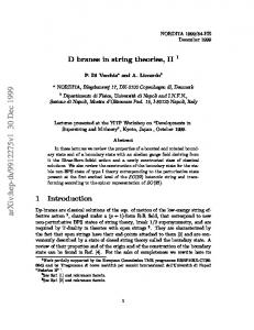
To understand the contribution to the amplitude by a given brane configuration, one can study perturbative string theory in the background of the branes at weak string coupling. For the D-branes this is straight forward, once one realizes that D-branes are space-time defects at which open strings can end.

open strings can end on D-branes

11 00 00 11 11 00 00 11

(Polchinski)

Figure 2: String in the background of a D-brane

Figure 2 shows this basic concept of D-brane physics. It was known since the early days of string theory that in open string theory one can as well impose Dirichlet boundary conditions (the end of the string is at a fixed position) as the usual Neumann boundary conditions (the end is free to move, no momentum is allowed to flow of the end). One usually neglected this possibility, since it introduced hyperplanes (the planes on which the endpoints are forced to stick) which break Lorentz invariance. It was the achievement of Polchinski to show [4, 5] via an explicit 1-loop open string calculation that these spacetime defects carry charge under the RR gauge fields of string theory and calculating their tension to be 1 TDp = p+1 (2.1) ls gs where ls and gs denote the string coupling and length respectively. These properties allow us to identify them with the stringy version of the solitonic solutions of SUGRA which I already called D-branes before. Now it is straight forward to do everything we are used to from perturbative string theory in the background of the D-branes. Quantizing the oscillator modes of the string 9

theory in the presence of the modified boundary conditions one finds that the massless spectrum of the open strings ending on the D-brane are given by a SYM multiplet living on the brane worldvolume. That is, for the D9 brane we find the usual N = 1 SYM multiplet consisting of the vector gauge field and the gauginos in 10d. All other branes yield dimensional reductions of those to the appropriate worldvolume dimension. Demanding conformal invariance on the string worldsheet yields equations of motion for the space-time fields by setting the β function of the 2d conformal theory on the worldsheet to zero, order by order in the string tension (which plays the role of the coupling constant in the 2d theory), just like in the well known case of Neumann boundary conditions. Writing down an action that yields these equations one obtains as an effective action for the D-brane theory a supersymmetric Dirac-Born-Infeld action with WessZumino couplings to the bulk fields [10] S = SDBI + SW Z = −

Z

q

dp+1ξ e−Φ −det(gij − Fij ) +

Z

dp+1ξ CeF

(2.2)

(r) where F = F − B, C = 10 is a formal sum over all the form fields present in r=0 C the IIA/B supergravity and the integral always picks out the right form to go with the right power of F from the exponential. The fields should be understood as pullbacks from superspace to the worldvolume. The low-energy approximation of this action, that is the expansion to lowest order in 2 ls (the string length), yields SYM on the worldvolume. This is in accordance with the analysis of the massless spectrum. The gauge coupling can be read off from (2.2) to be

P

gY2 M = lsp−3 gs .

(2.3)

As in the case of fundamental string theory the scalars on the worldvolume define the position of the brane in the transverse space. Via the DBI action these are coupled to the worldvolume gauge fields. This is an important property of the D-brane action which we will explain in more detail in the following. Basically a brane can absorb the flux of a charged particle by bending in transverse space, balancing the force from the gauge fields with its tension, that is with the worldvolume scalars. A flat D-brane breaks half of the supersymmetries (since the open string spectrum only has half of the supersymmetries of the closed spectrum). The supersymmetries preserved have to satisfy 1 ǫL = Γ0 · . . . · Γp ǫR

(2.4)

where the preserved supercharge is ǫL QL + ǫR QR and QL , QR are the supercharges generated by left- and right- moving degrees of freedom in the surrounding type II string theory. Choosing a non-trivial embedding generically breaks all the supersymmetries. If 1

which can e.g. be seen by analyzing the Killing spinor equations in the background of the D-brane soliton solution

10

the embedding geometry allows for some Killing spinors, lower fractions of supersymmetry may be preserved. If we try to repeat this analysis for NS5 branes we run into trouble. The NS5 brane metric looks like a tube, the dilaton blows up if we move towards the core and any conformal field theory description breaks down. Only asymptotically, the NS5 brane can be described by a well known conformal field theory, a WZW model [11]. The NS5 brane worldvolume theory is not accessible by purely perturbative string techniques. However we will see later that we can deduce its properties by string dualities.

2.3

D-branes and gauge theory

By now we have gained some insights in the dynamics governing D-branes. We have learned that there is a very deep connection between D-branes and gauge theories. We will analyse how some of the most interesting aspects of D-branes are captured by simple field theoretic phenomena. This discussion will pave the way for the discussion in the following chapters, where I will exploit the D-brane / gauge theory correspondence to learn about string theory as well as about gauge theory. The general philosophy is that we consider certain limits of string theory, in which the gravity and heavy string modes (the bulk modes) decouple, leaving us just with the open string sector described by SYM. The basic quantities that control this limit are the Planck scale Mpl and the string scale Ms (the inverse of the string length). They satisfy Mpl4 gs = Ms4

(2.5)

which just shows the relation between string frame and Einstein frame. Sending Mpl to infinity is the same as sending Newton’s constant to zero, so gravity is decoupled. Taking Ms to infinity sends all excited string states to infinite mass effectively decoupling them, too. This can be done at finite string coupling, keeping an interacting SYM theory.

2.3.1

Gauge theory on the worldvolume

As we have seen, the effective theory on the worldvolume is given by a DBI action. We want to analyse this world volume theory in the limit, where the bulk physics decouples, that is we get rid of gravity and other closed string modes. We only keep the degrees of freedom on the brane. Expanding the DBI action in ls2 (which explicitely shows up together with every F ) it is easy to see, that in the ls → 0 limit the theory on the worldvolume of the Dp-brane reduces to U(1) SYM in p+1 dimensions. The amount of supersymmetry preserved by a given brane is determined by its embedding in space-time, as discussed above. A flat brane always preserves half of the 32 supercharges of type II theory, leading to maximally supersymmetric Yang-Mills on the worldvolume. Now let 11

us consider what happens if N D-branes coincide. This situation was analysed by Witten [12]. A single D-brane supports on its worldvolume a single U(1) multiplet. These massless states arise from a string starting and ending on the same brane. The mass of a state is given by the length of the string times the string tension. The massless vector hence arises from a zero length string starting and ending at the same point. Each of the ends of the strings carries a Chan-Paton label of the gauge group, that is an index in the fundamental representation, so the vector multiplet is correctly left with a fundamental and an antifundamental index, an adjoint field. Clearly nothing happens to these states if many D-branes coincide. However, whenever two branes are close, there are new states that become important. Strings stretching from one brane to the other yield states whose mass is determined by the distance between the branes. They carry a fundamental Chan Paton index of the U(1) of the brane they start and end on respectively. It is natural to identify those as W-bosons of a broken U(2) gauge group. The distance between the branes determines the Higgs expectation value. When N branes coincide all the W-bosons become massless and the full U(N) gauge symmetry becomes visible. In order to obtain different gauge groups one can consider D-branes coinciding on top of space-time singularities. An example of such a singularity which is under control from perturbative string theory is an orientifold plane, the fixed plane of a Z2 orbifold action, that combines worldsheet parity with a space time reflection in r coordinates. The resulting p + 1 = 10 − r space-time fixed plane is called an Op orientifold plane. A similar calculation like that of Polchinski’s determination of the D-brane charge shows that the orientifold is also charged under the same RR field as the Dp, where the relative value of the charge is given by 2 qO = ±2p−4 qD .

(2.6)

The sign is determined by a discrete choice of the precise way one performs the projection. When N D-branes coincide on-top of the orientifold (and hence also coincide with their N mirrors), only oriented strings stretching between the branes will yield new massless gauge bosons, leading to an SO(2N) (USp(2N)) gauge theory on their worldvolume for an orientifold of negative (positive) charge. The best known example is the type I string. If we mod out IIB just by world-sheet parity we basically produce an O9. Since this is a space-filling brane we have to cancel the RR charge, forcing us to use the negatively charged orientifold with 32 D-branes on top of it, yielding an SO(32) gauge theory, as expected. 2

Here and in what follows I will always consider the D-brane and its Z2 mirror as different objects, each carrying charge qD . If one wants to consider only physical D-branes one should assign them charge 2qD in these conventions.

12

2.3.2

Compactifications and D-branes

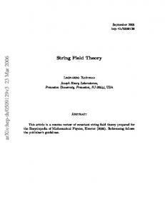
There is a seemingly different way that D-branes can be described by gauge theories. If we consider compactifications of string theory, we will have non-perturbative states in the resulting lower-dimensional theory from D-branes wrapping cycles of the compactification manifold. The mass of these states is just given by the tension of the brane times the volume of the cycle (and therefore has the 1/gs dependence signalling a non-perturbative state). At certain points in the moduli space of compactifications some of these cycles may shrink to zero size, leading to new massless states in the low-energy theory. Some of these states are usually massless vectors, giving rise to non-perturbative gauge groups.

cycle shrinks

Figure 3: Non-perturbative states from D-branes on shrinking cycles

2.4

Engineering Gauge theories

With the two mechanisms at hand we can try to engineer gauge theories, that is we make up a string theory geometry with branes that realize a certain gauge theory we want to study. Combining the two basic mechanisms discussed above in various ways there are several possibilities to do so. Basically all these different approaches described in the literature can be separated in three classes. As I will discuss in the last chapter they are actually equivalent. There I will also give a more technical discussion for the specific case of N = 2 theories in 4d.

2.4.1

Geometric Engineering

A geometric engineer tries to cook up a string background that captures all aspects of the gauge theory she wants to study in the geometry of the compactification manifold. In order to focus on the gauge theory modes, one has to decouple all stringy modes and all bulk modes. That is one has to send Ms and Mpl to infinity. Let me for simplicity of notation discuss the case of a K3 compactification ( see [13] and references therein), engineering an N = (1, 1) or N = (1, 0) supersymmetric gauge theory in 6d for type IIA 13

or the heterotic string respectively. It should be clear that these principles work the same way in other examples. The relevant scale is the 6d Planck scale given according to a KK ansatz by MP4 l,6 = VK3MP8 l,10 .

(2.7)

Decoupling gravity therefore effectively amounts to decompactifying the K3. Since the 6d gauge coupling of the perturbative gauge groups already present in 10d are also given via the KK ansatz as gY−2M,6 = VK3 gY−2M,10

(2.8)

they decouple in the same decompactification limit. The only gauge groups that survive are the non-perturbative gauge groups that arise via wrapping branes around vanishing cycles in the manifold. All information about the gauge theory is therefore encoded in the local singularity structure of the K3. The basic example is IIA on an ALE space, that is a non-compact version of K3. An ALE is a blow-up of an R4 /Γ orbifold, where Γ is a discrete subgroup of SU(2). Since spinors transform as a (2, 1) + (1, 2) under the SO(4) = SU(2) × SU(2) spacetime rotations, embedding the orbifold in just one of the SU(2) factors leaves half of the spinors invariant and hence also half of the supersymmetries unbroken. Since K3 can be written as an orbifold of T 4 , these orbifold singularities can arise locally in the geometry of K3. The statement that Γ should be a subgroup of SU(2) is equivalent to demanding that the holonomies of K3 only fill up SU(2) and not the full SO(4) of a generic 4d manifold. In order to obtain gauge dynamics, the local description in terms of the ALE is all we need. We expect new gauge dynamics when we move to the singular point, the orbifold itself. The ALE space has topological non-trivial cycles.

S1

Figure 4: Non-trivial 1-cycle on R2 /Z6. 14

Figure 4 illustrates non-trivial S 1 s arising from an R2 /Z6 orbifold. Similarly we get 2-spheres on the ALE. These 2-spheres shrink to zero size at the orbifold point. New massless states arise from D2 branes wrapping these cycles. The intersection pattern of the 2-cycles will determine the gauge group. Luckily all discrete subgroups of SU(2) can be classified by an ADE pattern, where the corresponding Dynkin diagram gives us precisely the information about the intersection numbers of the vanishing spheres. The resulting gauge theory has a non-abelian ADE gauge group.

2.4.2

Branes as Probes

“Branes as Probes” is the most natural way if we want to learn something about string theory from Yang-Mills theory. The idea is that in order to study what happens to a given string background once one takes into account all the quantum effects, one probes the background with a D-brane 3 . On the worldvolume of the D-brane we will as usual find a gauge theory. The background geometry will be encoded in this gauge theory via the matter content, the amount of unbroken supersymmetry and the interaction potentials. Solving the quantum gauge theory will teach us about the quantum behaviour of the background. This technique has been very successfully used for probing Dp+4 branes and Op + 4 planes with Dp branes [14, 15, 16, 17, 18], as well as probing orbifold singularities with Dp branes [19, 20]. In both cases the matter content and classical superpotential of the gauge theory can be analyzed by perturbative string theory. For the higher p branes, we will find new states on the Dp worldvolume corresponding to the zero modes of strings stretching between Dp and Dp + 4 branes in addition to the gauge multiplet already present from the Dp-Dp strings. In the case of the orbifold we first include all the twisted sectors required in string theory for consistency by including all the mirror D-branes and strings stretching in between them. Then we project onto states invariant under the orbifold group and this way obtain the corresponding spectrum.

2.4.3

Hanany-Witten setups

Hanany and Witten (HW) introduced a setup of intersecting branes realizing d = 3 N = 4 gauge theories. The gauge theory again lives on the worldvolume of D-branes. The other branes make the gauge theory interesting by breaking SUSY and introducing new matter. Since we are now only dealing with flat branes in flat space, many things become very intuitive. Moduli and parameters just correspond to moving the branes around and are very easy to visualize. As advertised above I will show in the end, that 3

In this language one could view string theory as we used to know it as probing space-time with a fundamental string.

15

all the 3 approaches are actually equivalent, so by studying the intuitive HW setups we can get non-trivial results about quantum string backgrounds by considering the “dual” branes as probes setup. The next chapter is devoted to an extensive review of the HW idea, so I won’t go into any details at this point.

2.5 2.5.1

D-branes and dualities String Dualities and M-theory

Probably the most important application of D-branes so far is the idea of string-dualities, the statement that one and the same physical system has two dual descriptions. The concept of duality was already discussed long ago in the context of field theories, as I will explain in more detail in the Chapter 3. In string theory duality was first detected in the form of T-duality [21]. Studying the spectrum of bosonic string theory on a circle of radius R 1 H = p2R + p2L + oscillators 2 R 1 ls pR = √ ( n − m) ls 2 R 1 ls R pL = √ ( n + m) ls 2 R

(2.9)

One sees that due to the presence of winding modes characterized by the integer m as well as momentum modes n around the circle, the states are invariant under an exchange of the two if one simultaneously takes R into ls2 /R. This invariance under R → 1/R exchange can be shown to be a symmetry of amplitudes to all orders in perturbation theory and is believed to be valid even non-perturbatively. The two compactifications are T-dual to each other. For the superstring this T-duality works almost the same. For example type IIA on R is dual to IIB on ls2 /R. In this case the p + 1 form fields from the RR sector T-dualize into p + 2 and p form fields, depending on whether we take the components along or transverse to the compact direction. Since the Dp branes couple to these fields, T-duality transverse to the worldvolume produces a Dp + 1 brane while T-duality along a worldvolume direction leaves us with a Dp − 1 brane. More interesting are dualities relating one string theory at weak coupling to another string theory at strong coupling. Many dualities of this type have been discovered over the recent years. However non of them can be proven by a direct calculation. Since by definition we compare a strongly coupled with a weakly coupled theory, only one side is accessible to calculations. Duality then amounts to a prediction for the strong coupling behaviour of the other theory. The reason why most string theorists nevertheless 16

believe in the validity of these dualities is that they can be checked in several ways. The most important check is the matching of objects which are BPS. They preserve some fraction of the supersymmetry and are therefore protected by the superalgebra from any renormalization. We have already encountered some of these objects: D-branes. This way certain properties of these non-perturbative states which dominate the strong coupling theory can be calculated and they can be matched onto the perturbative states at weak coupling. One of the examples I am going to consider several times in this work is the selfduality of type IIB string theory. Type IIB with coupling gs is dual to type IIB with 1/gs . a Including the axion a we can build a complex coupling τ = 2π + gis . Combining the gs to 1/gs duality with the invariance of the axion under shifts of 2π, a whole SL(2, Z) of dual theories can be constructed. The NS 2-form field combines with the RR 2-form into an SL(2, Z) doublet. The objects coupling to them, the fundamental F1 and the D1 string are exchanged under the strong-weak coupling duality. More general SL(2, Z) transformations take the F1 into a (p, q) bound state of p fundamental and q D-strings. Similarly their magnetic duals, the NS5 and the D5 brane form an SL(2, Z) doublet. Since there is only one 4-form field, it has to be a singlet under SL(2, Z) and hence the D3 brane stays invariant under all duality transformations. Since the low-energy effective actions of the dual theories are supposed to agree, the Planck scale has to remain invariant, therefore using (2.5) the dual string scale has to be Ms gs1/2 . Basically all string dualities can be summarized as the existence of an conjectural 11d theory, called M-theory, which contains all the string theories as well as 11d SUGRA as perturbative expansions in certain limits.

IIB 11d SUGRA het SO(32) IIA M

het E8 x E8

type I

Figure 5: All known string theories as well as 11d SUGRA are just different perturbative expansions of an overarching 11d M-theory. 17

Since I am going to use this M-theory picture in what follows, let me briefly present as a defining duality of M-theory the duality between 11d SUGRA and type IIA, which originally led to the discovery of M-theory [6, 22]. According to this proposal M-theory on a circle is type IIA string theory with the IIA coupling and string length given in terms of the 11d Planck length and the radius of the 11th dimension R as gs2 =

3 R3 2 lpl l = s 3 lpl R

(2.10)

These relations can be obtained by comparing the low-energy effective actions. The relation really constitutes a strong-weak coupling duality: at very large R IIA becomes strongly coupled and we lose all control. However in the 11d picture as R becomes bigger the curvature becomes smaller and SUGRA becomes a good approximation. Similar at very small R the curvatures are Planckian in 11d, so SUGRA fails to capture the physics, however perturbative string theory is a good description. To describe couplings of order 1, we need the yet unknown full fledged M-theory. The appearance of the 11th dimension can be seen from studying D-branes. D0 branes are non-perturbative states, whose mass goes to zero in the strong coupling limit. N D0 branes are believed to form a unique threshold bound state (that is with zero binding energy) [12, 23]. They therefore led to a tower of states with mass gN . It is natural to s ls identify these as momentum modes around the 11th dimension of radius R = gs1ls . Mtheory also provides us with a nice organization principle for all the other branes. From 11d SUGRA we learn that M-theory has two extended objects, the M2 and the M5 brane. Together with three more complicated solutions that only arise upon compactification of at least one more direction, the wave (momentum mode around the circle) with mass 1/R, 9 its magnetic dual, the KK monopole 6 brane with tension R2 /lpl and an M9 brane with 3 12 tension R /lpl , they give rise to all brane solutions in the perturbative limits of M-theory.

2.5.2

Matrix Theory

Having said the above, it would clearly be desirable to find a microscopic definition of Mtheory. The only candidate that has emerged so far is matrix theory [8]. The idea behind this approach is to quantize the theory in a special frame, called the infinite momentum frame, where only a very limited amount of the original degrees of freedom are visible. What we do is boost ourselves as observers infinitely along a compact direction, so that of all modes with momentum N/R only those with positive N survive. This has to be considered as N and R both go to infinity with N/R also going to infinity. Since we want to work at finite N to do any realistic computation, one would like to study a reference frame that is described by finite N matrix theory and reduces to the IMF in the N → ∞ limit. Such a frame exists, the discrete light cone frame. Therefore we want to study discrete lightcone quantization (DLCQ) of M-theory. This was conjectured 18

to be described by the finite N matrix model in [24]. DLCQ formally can be thought of as quantizing the theory on a compact lightlike circle. This notion seems to be rather counterintuitive. Indeed it was shown in [25] that the best way to think about the DLCQ is to consider it as a limit of a compactification on an almost lightlike circle, that is !

!

x x + ∼ t t

q

R2 2

+ Rs2

− √R2

!

!

x + ≈ t

R √ 2

2 ! √Rs 2R − √R2

+

(2.11)

where Rs > R2 . All KK states, the fermions and the q scalars become very massive in this limit, the lightest ones being the scalars with 2 mass R ·1/R1 . However due to the exponential suppression in (4.4) for sufficiently small R1 R2 /R1 the QCD scale will be much smaller than any of the other masses in the problem, leaving us with pure QCD as advertised. Note that this limit corresponds to very weak coupling in (4.3). This is not surprising, since as discussed above, (4.3) determines the coupling at the energy scale, where all the other fields become important. We want this to happen far above the QCD scale, that is at very weak coupling due to asymptotic freedom of QCD. A second very important application is to study the deformations of the fixed points. As we will see in what follows this can be done very easily using branes. A given brane setup represents a certain phase of string theory. This will become more transparent once we have shown that brane setups are actually equivalent to the language of geometric compactifications. By tuning parameters of this compactification, that is by moving around the branes, we encounter critical points as certain branes collide, the non-trivial FP. Often at the FP we see new deformations that allow us to perform a phase transition into a topologically distinct vacuum of string theory. Last but not least these FP theories play an important role in the recent matrix conjecture [8]. As explained in Chapter 2 this conjecture elevates the correspondence between gauge theory and non-perturbative string theory to a principle, defining all of Mtheory in terms of the world-volume theory of certain branes. For Matrix compactifications on a T 4 the relevant brane theory is the strong coupling limit of the worldvolume of N coinciding D4 branes, that is the worldvolume theory of N M5 branes: the (2,0) FP theory [27].

4.2.2

Physics at non-trivial FP from branes

General idea From what we have learned so far it should be clear that branes are the essential tool to prove the existence of strongly coupled fixed points in 5 and 6 dimensions. The principal idea is as follows: one considers string theory in the background of certain branes. Since this is a well defined theory, we can try to take the limit in which gravity and the other bulk modes decouple. In some cases this leaves us with an interacting theory on the brane. The strong coupling limit then corresponds to having some branes coincide, usually exhibiting an infinite tower of states becoming massless as we would expect from a conformal field theory. So proving the existence of an interacting fixed point amounts to analyzing whether string theory allows for a decoupling limit that leaves an interacting theory on the branes. To demonstrate this procedure let us briefly consider the brane realization of the (2,0) fixed point that was found by [76] using a geometric picture. 48

I will also discuss the maximally supersymmetric cases in 5,7 and higher dimensions as well as in 6d with (1,1) supersymmetry. In these cases the analysis of [77] tells us that there are no superconformal algebras. Indeed we will find in the brane picture that in these cases decoupling of the bulk modes leads automatically to a free theory on the brane. The (2,0) theory from the M5 brane Consider a system of N parallel M5 branes. In the same spirit as in (3.2) we want to decouple bulk gravity by taking the limit Mpl → infinity. We want this to do in such a fashion that the theory on the M5 branes stays interacting. Recall that the theory on the M5 is that of N N = (2, 0) tensor multiplets. This theory does not have a coupling constant which we could keep fixed. However we do know that these tensor multiplets couple to the strings that describe the ends of M2 branes. The tension of these strings is lD3 pl where D is the characteristic distance between two M5 branes. These tensions correspond to the vevs of the scalars in the tensor multiplet, since they are given by the M5 positions and have mass dimension 2 in the natural normalization. Therefor the decoupling limit will be D → 0, lpl → 0, holding u = lD3 fixed. At the origin of the moduli space, that pl is if all the u go to zero, we expect a superconformal fixed point. The strings become tensionless and provide the continuum of massless states of the conformal theory. One might worry that this fixed point could be a free theory. One way to see this cannot be the case is to consider the theory on a large circle R. The resulting theory will be 5d SYM with gauge coupling gY2 M = R 3 . We see that this is an interacting theory and the large R limit even corresponds to very strong coupling. d=6 N=(2,0) 5 brane

2 brane string on 5 brane

tensionless string continuum of massless modes

Figure 10: Brane realisation of the (2,0) theory.

3

One way to see this relation is to consider the compactification in terms of branes. The M5 turns into a D4 with gY2 M = ls gs = R.

49

The other maximally supersymmetric theories One can try to do a similar construction for SYM theories in 5,6,7 and higher dimensions, which are also maximally supersymmetric (where this time in 6d we have non-chiral (1,1) supersymmetry). These can be realized as the world volume theories of D4,5,6 and higher branes. We want to send Mpl and Ms to infinity in order to decouple all bulk modes 4 . If we would again predict non-trivial FPs we would be in trouble since the analysis of [77] shows that for these cases there are no superconformal algebras. We expect a non-trivial theory once we put several branes on top of each other. N colliding branes give rise to U(N) gauge theory. In order to obtain an interacting theory on the branes we need to keep gY2 M on the branes finite. According to (2.3) gY−2M = Msd−3 /gs for the d+1 dimensional gauge theory on the worldvolume of a Dd brane. Since Ms4 = gs Mpl4 We see that for the D7 brane gY−2M = Mpl4 and hence gY M goes to zero in the decoupling limit Mpl , Ms → ∞. This still is true in higher dimensions. We are left with a free theory! For the D6 gY−2M = Mpl3 /gs1/4 we see we can keep gY M finite if we simultaneously with Mpl take gs to infinity. According to [6] strongly coupled IIA string theory is better thought of as 11d SUGRA. The duality tells us that the 11d Planck scale Mpl,11 is given by 3 Mpl,11 = Mpl3 /gs1/4 = gY−2M . In order to decouple the 11d bulk we again have to stick to a free theory on the worldvolume. For the D5 and D4 branes a similar story is true. In both cases gY2 M can be kept finite only in the strong string coupling limit. S-dualizing, the D5 brane turns into an −2 2 NS5 brane at weak coupling with gauge coupling gN S5 = Ms which is again free in the decoupling limit. One can slightly modify the decoupling limit by relaxing the condition that Ms is supposed to go to infinity. In this case still all the bulk modes decouple. However we are no longer left with just SYM on the brane. But whatever it is we are left with, string theory tells us that it exists. This way Seiberg proved [28] the existence of a 6d string theory. It has a string scale Ms and hence does not correspond to a conformal theory. For the D4 brane the strong string coupling limit once more decompactifies the 11th dimension. The D4 brane becomes an M5. Hence the 5d SYM at strong coupling grows an extra dimension. We do obtain a non-trivial strong coupling fixed point, but it is again the 6 dimensional (2,0) theory which we encountered before. 4

The former is required to decouple gravity while the latter decouples the higher order terms from the DBI action.

50

4.2.3

6d Hanany-Witten setups

Motivation In order to study less supersymmetric theories we need more involved brane setups. In what follows I will present a Hanany-Witten setup describing fixed points in d = 6 with N = 1. This setup was presented in [80] and further analyzed in [81, 71, 82]. The same fixed points where analyzed from the branes as probes point of view by [83, 20] and were geometrically engineered from F-theory in [84]. The motivation for analyzing these theories instead of their more supersymmetric cousins is threefold. • As described above we can learn about 4d gauge theory by putting these fixed points on a torus. Since the dynamics of maximally supersymmetric SYM in 4d is rather constrained it is definitely interesting to do this with less supersymmetric theories. If we again want to study non-supersymmetric QCD by imposing antiperiodic boundary conditions on the fermions, we have this time the choice to put different boundary conditions on fermions coming from vector and hypermultiplets, opening up the possibility to realize QCD with matter. • The (2, 0) fixed point has only one possible deformation, which corresponds to moving the M5 branes apart. To really study phase transitions we need to study the more elaborate fixed points with only 8 supercharges, which in general do allow several different perturbations, leading to a transition between distinct phases. • When used as matrix models these fixed points should be used to describe DLCQ string theories with 16 supercharges, like the heterotic string on a T 4 or type II string on a K3. These theories have a much richer dynamics and are hence more interesting than their more supersymmetric cousins. The consistency requirement: Anomaly cancellation As discussed above, even though field theory is not the right arena to discuss the appearance of non-trivial FPs, it nevertheless imposes several constraints on the existence of consistent strong coupling limits. In 6 dimensions this criterion is anomaly cancellation. Let me briefly review the relevant mechanism from the field theory point of view. In what follows we will see that the branes actually know about this mechanism and only yield anomaly free theories. The anomaly in six dimensions can be characterized by an anomaly eight form. For Q a theory with a product gauge group G = α Gα with matter transforming in the representation R, the anomaly polynomial reads I=

X α

TrFα4 −

X R

!

nR trF 4 − 6 51

X

αα′

RR′

nR,R′ trR Fα2 trR′ Fα2′ .

(4.5)

Here, Tr denotes the trace in the adjoint and trR is the trace in Representation R. The symbol tr is reserved for the trace in the fundamental representation. nR denotes the number of matter multiplets transforming in a particular representation R and nRR′ is the number of multiplets transforming in the representation R × R′ of a product group Gα ×Gβ . For a consistent theory, the anomaly should be cancelled in some way: Either the anomaly polynomial vanishes or we cancel the anomaly by a Green–Schwarz mechanism [85]. So let us look at the anomaly in more detail. First, we want to rewrite the anomaly polynomial using only traces in the fundamental representation. Formally, the polynomial then looks like    X X I= cα α′ trFα2 trFα2′ aα trFα4 + (4.6) α

αα′

For concreteness let me discuss the case of a single gauge group factor. The anomaly reduces to I = atrF 4 + c(F 2 )2 (4.7)

For a = c = 0 the anomaly cancels completely. If a 6= 0 the anomaly can’t be cancelled and the theory is sick. However if a = 0 we can cancel the anomaly by the Green-Schwarz mechanism by coupling it to a two-index tensor field. In 6 dimensions the tensor splits into an anti-selfdual and an selfdual part. While the former sits in the gravity multiplet, the latter is part of the tensor multiplet. Depending on the sign of c we have to use one or the other. If c > 0 we can cure the anomaly by coupling to a tensor multiplet, for c < 0 the theory is sick without coupling to gravity. If realized in terms of branes, in the latter case there can’t be a consistent decoupling of the bulk modes. For a very detailed discussion of the anomaly polynomials for product gauge groups see e.g. [86]. In the case of SU(N) gauge theory using the group theoretical identity [87] 

4 4 2 TrFSU (N ) = 2NtrFSU (N ) + 6 trFSU (N )

we find that 4



I = (2N − Nf )trF 4 + 6 trF 2

2

.

2

(4.8) (4.9)

Therefore, the deadly F term cancels precisely for Nf = 2N. The prefactor c of the 2 (F 2 ) term is always bigger than zero, so that we can cancel the anomaly by coupling to a single tensor multiplet. Adding the Green-Schwarz counterterm, the action contains a coupling of the scalar φ in the tensor multiplet to the gauge fields, so that the gauge kinetic term becomes [17] √ 1 2 2 trFµν + cφtrFµν . 2 g We see that one can absorb the bare gauge coupling into the expectation value of φ by just a shift of the origin. We obtain an effective coupling √ 1 = cφ. 2 gef f 52

At φ = 0 we expect the possibility of a strong coupling fixed point [17]. The brane configuration In order to study Hanany-Witten setups in 6 dimensions, we need as fundamental ingredients D6 branes, on whose worldvolume we realize the gauge theory. In addition one has the obligatory NS5 branes, between which the 6 branes are suspended. As usual this compact interval gets rid of one of the 7 worldvolume dimensions of the D6 brane via KK reduction. In addition the boundary conditions for the D6 branes ending on the NS5 branes projects out some of the fields. In total we break 3/4 of the supercharges (1/2 by the D6 and another 1/2 by the NS5) leaving N = 1 in d=6. As usual there are two ways to introduce flavors in the setup. One is to include the additional flavor branes, which in our case will be D8 branes. I will explain how to deal with them later. For now I will include flavors via semi-infinite D6 branes to the right and left. With this the players in our game are:

NS 5 D6 D8

x0 x x x

x1 x x x

x2 x x x

x3 x x x

x4 x x x

x5 x x x

x6 o x o

x7 o o x

x8 o o x

x9 o o x

The presence of these branes breaks the SO(9, 1) Lorentz symmetry of type IIA down to SO(5, 1) × SO(3) corresponding to rotations in the 789 space and Lorentz transformations in 012345 space. The SO(3) can be identified with the SU(2) R-symmetry of the d=6 N = 1 SUSY algebra. To understand the basic issues that are different in 6d from the “usual” Hanany-Witten setups discussed above let me first focus on the simplest setup. 7,8,9,10

6

L

N

R

Figure 11: The brane configuration under consideration, giving rise to a 6 dimensional field theory. Horizontal lines represent D6 branes, the crosses represent NS5 branes. 53

Figure 11 shows a configuration of N D6 branes suspended between two NS5 branes. There are L (R) semi-infinite D6 branes to the left (right). Let us first discuss the matter content corresponding to this setup. As usual we get an SU(N) vector multiplet from the color branes and L + R fundamental hypermultiplets from the semi-infinite flavor branes. But these are not all the matter multiplets we get. According to our standard philosophy we keep all the light modes coming from the lowest dimensional branes. In all other dimensions this meant decoupling the worldvolume fields of the NS5 branes. But here the NS5 branes live inside the D6 brane, they also have a 6d worldvolume as the finite D6 brane pieces we are considering. Hence we should also include the matter from the NS5 branes. This can also be discussed in a more quantitative manner, looking at the precise decoupling limit. As discussed in our introduction to Hanany-Witten setups we want to take Mpl and Ms to infinity in order to decouple the bulk, sent the length L of the interval to zero in order to decouple the KK modes and do this all in such a way to keep the gauge coupling of the 6d theory fixed. According to (2.3) we get gY2 M = Mg3sL . s The theory on the NS5 branes is a theory of tensor multiplets, so there is no gauge coupling. To see what is going on let us translate into 11d units via (2.10). We see that l3

. But this is precisely the tension of the M2 branes stretching between the 5 gY2 M = pl,11 L branes. When discussing the decoupling of the (2,0) theory we found that this quantity basically governs the interaction strength of the theory on the 5 brane. Keeping it fixed means that we should indeed keep the interacting modes on the 5 branes as well as those on the worldvolume of the finite D6 brane. So now what is this additional matter? The theory on a IIA NS5 brane is the theory of a (2,0)– tensor multiplet. This multiplet consists of a tensor and 5 scalars (and fermions). Because of the presence of the D6 branes, one half of the SUSY is broken and we are left with a (1,0) theory. The tensor multiplet decomposes into a (1,0) tensor, which only contains one scalar, and a hypermultiplet, which contains 4 scalars. The hypermultiplet is projected out from the massless spectrum because the position of the semi-infinite D6 branes fixes the position of the NS5 branes. Moving the NS5 brane out of the D6 brane (remember that we have the 5 brane embedded in the D6 brane) corresponds to turning on the 3 FI terms and a theta angle. The scalar in the tensor multiplet corresponds to motions of the 5 branes in the x6 direction. This is going to be a modulus of our theory. We have two NS5 branes and therefore two tensor multiplets, but effectively we keep only one of them because one of the scalars can be taken to describe the center of mass motion of the system. The vev of the other scalar gives us the distance between the NS5 branes. On the other hand, we know that the distance between the NS5 branes is related to the inverse Yang-Mills coupling of the six-dimensional gauge theory according to the usual KK philosophy. The vev of the scalar hence plays the role of a gauge coupling, as expected from field theory. 54

Now let us turn to the quantum picture. As in the other theories with 8 supercharges, the 1-loop information will be encoded in the bending of the NS5 branes and there won’t be any further corrections. We in particular expect the bending to provide us with the information about the anomalies, since those are a 1-loop effect. Indeed the analysis of the bending is really easy in 6d, as discussed before. Since the NS5 branes are embedded in the D6 branes there is no transverse worldvolume. The NS5 brane can’t absorb any flux coming from the charged ends of a D6 brane. The only way we can have a consistent brane setup is if the net charge cancels. The net charge is given by the number of D6 branes ending from one side minus the number of D6 branes ending from the other side. Thus, we only get a consistent picture if: N = L = R, where L (R) denotes the number of D6 ending from the left (right). The total number of flavors is Nf = L + R = 2N. (4.10) Together with the tensor multiplet from the NS5 branes this is indeed the (only) right matter content to cancel the anomaly.

5

Realization of the fixed point Our theory has a Coulomb branch parametrized by the vev of the scalar in the tensor multiplet. At the origin, the effective gauge coupling becomes infinite and we find the strong coupling fixed point. Since the tensor multiplet corresponds to the distance between the NS5 branes this happens precisely when they coincide. The strings from D2 branes stretching between the NS5 branes become tensionless. Building product groups is straight forward. Again we find FPs whenever the NS5 branes coincide. An interesting generalization is to put the theory on a circle. In this case we will see an SU(N)k gauge group, where k denotes the number of NS5 branes. Tuning the moduli in such a way that we obtain the fixed point theory amounts to moving all the 5 branes on top of each other. Since the distance between the 5 branes is the effective coupling constant of the corresponding gauge theory we see that there is always one gauge group who’s color branes stretch around the entire circle, no matter where we choose to bring our 5 branes together. This means that we will always have one gauge factor with a finite gauge coupling that becomes free in the IR and hence becomes a global symmetry. From the field theory point of view this statement can also be seen to be true. Defining 5

For SU (2) and SU (3) there are also some other possibilities since they do not have an independent fourth order Casimir and hence a vanishes automatically. Global anomalies [88] restrict us to Nf = 4, 10 for SU (2) and Nf = 0, 6, 12 for SU (3). The 10 flavor case can be achieved by realizing SU (2) as U Sp(2) with an orientifold. The other SU (3) theories do not have an HW interpretation.

55

the effective gauge couplings by absorbing the classic gauge couplings in the vev of the scalars in the tensor multiplets, one finds that there is always one subgroup for which gef f becomes negative at large φ [20], so that we should start of with a finite value for this coupling. −2 R6 R6 The value of φ at which this sign change happens is given by gdec.f act. = l3 gs = l3 s

pl,11

(remember that φ has mass dimension 2). That is in the decoupling limit, where we send lpl,11 → 0 keeping l3Lgs fixed, this critical value goes off to infinity, so we do not see any s effect of the finite radius. If however we choose to also send R6 to zero as well, keeping R6 fixed, we can engineer a theory with the following properties: l3 pl,11

• it decouples from all bulk modes, hence it is 6d • gauge theory breaks down at energy scales important

R6 , 3 lpl,11

new degrees of freedom become

• the theory contains string like excitations with tension

R6 3 lpl,11

One usually refers to those theories as little string theories. The way we constructed them is the T-dual of the original construction of [89] as a generalization of Seiberg’s work [28] on the theory with 16 supercharges. Including 8 branes So far we have seen how to realize fixed points in branes. Now I will move on to more complicated setups in order to classify all fixed points realizable by HW setups. In [90] all anomaly free matter contents in 6d have been classified. Strictly speaking this list should be seen as the list of all theories that could possibly have a consistent strong coupling fixed point. The nice stringy result is that indeed all of them do. HW setups will not be able to generate the exceptional gauge groups, but will be very efficient at classifying those FP allowed with classical gauge groups and products thereof. The few missing cases can be realized via geometry [84, 91]. In order to build more general fixed point theories, let us now look at the second possibility to include flavors, via D8 branes living in 012345789, as discussed in [71]. D8 branes introduce additional complication, since D8 branes are not a solution of standard IIA theory but require massive IIA [92], that is the inclusion of a cosmological constant m. The D8 branes then act as domain walls between regions of space with different values of m. m is quantized and hence in appropriate normalization can be chosen to be an integer. The presence of m makes itself known to the brane configuration via a coupling −m

Z

dx10 B ∧ ∗F (2) , 56

(4.11)

where B is the 2 form NS gauge field under which the NS5 brane is charged and F is the 8 form field strength for the 7 form gauge field under which the D6 is charged. From the Bianchi identity for the 2 form field strength dual to F (8) in the presence of a D6 brane ending on a 5 brane, dF (2) = d ∗ F (8) = θ(x6 )δ (789) − mH (where H = dB), one gets mdH = δ (6789) . The δ function comes from the charge of the D6 brane-end. From here we get back the old result, that for m = 0 D6 branes always have to end on a given NS5 brane in pairs of opposite charge (that is from opposite sides). However for arbitrary m this relation shows that RR charge conservation requires that we have a difference of m between the number of branes ending from the left and from the right 6 . n

L

N

R

m=p

m=p+n

Figure 12: Basic Hanany Zaffaroni Setup

Figure 12 shows the basic brane configuration involving D8 branes. The n D8 branes in the middle give rise to n flavors for the SU(N) gauge group. In addition they raise the cosmological constant m from p to p + n. In the background of these values of m the modified RR charge conservation tells us N = L−p

R = N − (p + n)

With the R + L flavors from the semi-infinite D6 branes the total number of flavors is L + R + n = 2N still in agreement with the gauge anomaly considerations on the 6 brane for every possible value of p. So far we have not succeeded in obtaining any new FPs, since SUSY QCD with Nf = 2Nc is just what we were already able to realize with semi-infinite D6 branes. However as we move on we will need the D8 branes in more elaborate setups. 6

Throughout this work I will use the following conventions to fix the signs: by passing through an D8 from left to right m increases by 1 unit. In a background of a given m the number of D6 branes ending on a given NS5 from the left is by m bigger than the number of D6 branes ending from the right.

57

Orientifolds There is one more element we can incorporate in the HW brane setup, the orientifold. Since an orientifold breaks the same supersymmetries as the corresponding D-brane, we can introduce O8, O6 or both. Each of them comes with two possible signs. Let us first consider the O8. We have to distinguish two possibilities: O8 planes with negative or positive D8 brane charge (that is -16 or +16) [4]. The former are the T-dual of the O9 projecting IIB to type I. On the D8 worldvolume they project the symmetry group to a (global) SO group, while on the D6 we get a local USp group. The positively charged O8 projects onto global USp and local SO. If we want to have vanishing total D8 charge, we should restrict ourselves to either 2 negatively charged O8s with 32 D8 branes or one O8 of each type. There is indeed a physics reason that we should restrict ourselves to satisfy this requirement. What becomes important is that not only the cosmological constant jumps when we cross a D8 brane, but also the dilaton. If the dilaton is constant to the right of a given D8 brane, e−Φ (the inverse string coupling) will rise linearly on the left. For symmetry reasons this means that the dilaton will run with slope -8 into an O8 from the left and leave with slope +8 on the other side. In order to be back to slope -8 again before hitting the next O8, one has to put precisely 16 physical D8 branes in between. One interesting application of this behaviour is that this way the coupling may diverge at the orientifold planes, while it is finite everywhere else and even constant in between the 8th and the 9th physical D8. Usually one refers to this whole setup as type I’ string theory. Of course it is no problem to include just one O8 and fewer D8 branes by just keeping far away from the others.

m=8

m=-8

K

K+8

Sp

m=8

m=8

m=-8 K

SU

K-8

SO

m=-8

m=-8

SU m=8 K

K

SU + Asym.

SU + Sym.

Figure 13: Various possibilities to introduce O8 planes

The gauge groups corresponding to brane setups in Figure 13 have been analyzed in 58

the equivalent setup for 4d in [50]. If the O8 is in between two 5 branes the ‘center’ gauge group is projected to USp(K) or SO(K) respectively. All other gauge groups stay SU, however the SU groups to the right are identified with those to the left and one effectively projects out half of the SU groups. In addition to this, in 6d we get the special situation that the O8 also changes the cosmological constant. For symmetry reasons we have to choose m = ±8 on the two sides of the orientifold. Therefore we obtain in total USp(k) × SO(k) ×

Y

SU(k + 8i)

or

i

Y i

SU(k − 8i)

respectively. From strings stretching in between neighbouring gauge groups we get bifundamentals ( , ). We have taken all the D8 branes that are required to cancel the O8 plane charge to be far away. Of course including them we get some more fundamental matter fields and new contributions to the cosmological constant. The other possible situation considered in [50] is that one of the 5 branes is stuck to the O8. In this case all the groups stay SU, again with the left and the right ones identified, leading to effectively half the number of gauge groups. In addition the middle gauge group has a matter multiplet in the antisymmetric or symmetric representation for positive/negative charge O8 planes. In 6d we again have the effect of the cosmological constant and as a result get Y SU(k ± 8i) i

with antisymmetric/symmetric tensor matter in the first gauge group factor in addition to the bifundamentals. The other realization of SO and USp groups is to introduce an O6 along the D6 branes. In discussing O6 planes we have to be careful to take into account an effect first discussed in [93]: whenever an O6 passes through an NS5 brane, it changes its sign. Originally this was argued for O4 and NS5 based on consistency of the resulting 4d physics. Here we could basically do the same: without including this effect on would construct anomalous gauge theories. The sign flip miracously removes all anomalies, providing strong arguments in favor of this assumption. There also exist some worldsheet arguments, that further support the existence of the flip [94]. Due to this sign flip the O6 also contributes to the RR charge cancellation. Since its charge is +4 on one side and -4 on the other, the number of D6 branes ending to the left and right also has to jump by 8. We therefor are left with product gauge groups forming an Y SO(N + 8) × USp(N) i

chain with bifundamentals. Bringing the 3 ingredients - D8, O8 and O6 - together, we can 59

clearly cook up very complicated models. I will write down some hopefully illustrative examples later on. All these gauge theories I constructed with the help of orientifolds are anomaly free [86, 90, 83] upon coupling to the tensor multiplets associated to the independent motions of the 5 branes. Note that in the case of the O8, already a single NS5 brane gives rise to a tensor multiplet, parametrising the distance to the fixed plane. There is no decoupled center of mass dynamics since presence of the orientifolds breaks translation invariance along the 6 direction. Again it is straight forward to put the theory on a circle. I will restrict myself to the discussion of O8s. The O6 case is pretty obvious. The only thing one has to take care of is that only an even number of NS5 branes is allowed, so that the “global” groups from semi-infinite D6 branes are either both USp or both SO and we are able to close the circle. We should either take 2 negatively charged O8s with 32 D8 branes (that is the 16 physical D8 branes and their 16 mirrors) or a pair of oppositely charged O8s. 16 D8

16 D8

m=-8

m=8

K+16 O8

K+16 K+8 K

K

K+8

m=8 m=-8 O8

Figure 14: Brane configuration yielding a product of two USp and several SU gauge groups with bifundamentals and an antisymmetric tensor.

Encoding the position of the D8 branes in a vector wµ , where the entries in w denote the number of D8 branes in the gauge group between NS5 brane number µ and number P µ+1, one can write down formulas for the resulting gauge groups. Clearly µ wµ = 32. In addition we introduce a quantity Dµ that encodes in a similar way the information about 60

the orientifold: the entry corresponding to the gauge group that includes an orientifold is 16, since an O8 carries 16 times the charge of a D8. All other entries are zero. Let me only discuss the case of 2 negatively charged O8s with 32 D8 branes. This will have a dual description in terms of SO(32) small instantons. The case of oppositely charged orientifolds describes a disconnected part of the moduli space. It is dual to string theory compactifications with reduced rank of the gauge theory, like the CHL string [95]. We have to distinguish three cases • the number of NS5 branes is odd, so one of them has to be stuck at one of the O8s and the others live in mirror pairs on the circle • the number of NS5 branes is even, one is stuck at each of the orientifolds and the others appear in mirror pairs • the number of NS5 branes is even and all of them appear in mirror pairs on the circle and are free to move Let me discuss in some detail the case where k + 1, the number of NS5 branes, is odd. The other two cases can be worked out the same way [81, 83]. As in Figure 14 we have two orientifolds on the circle, both with negative charge. An example also explaining the notation is illustrated in the following figure: w4

w5=w2

w3

5

4

m=-8+w0+w1+w2

3 6

O8

2K+16-2 W0-w1

2 m=8

m=-8

m=-8+W0

2K

1

0

w2 m=-8+W0+w1

w6=w1 w1 W7=W0

O8

W0

w0=W0+W7=2 W0

Figure 15: Notation in the example of 7 NS5 branes on the circle 61

One of the 5 branes is stuck on the one orientifold. We label the 5 branes with µ running from 0 to k as in Figure 15 7 . In addition there are 32 D8 branes. Let again wµ denote the number of 8 branes in between the µth and (µ + 1)th NS5 brane. Obviously P µ wµ = 32. Also symmetry with respect to the orientifold plane requires wµ = wk+1−µ . It is useful to slightly modify the definition of the vector counting the D8 branes by introducing Wµ in order to take care of the effect that for every gauge group whose color branes stretch over the orientifold half of the wµ branes have to be located on either side. Therefore in these cases we define Wµ = 21 wµ while in all other cases Wµ = wµ . According to the rules of how to introduce 8 branes and orientifolds 8 , we find that the gauge group is k/2

USp(V0 ) ×

Y

SU(Vµ )

(4.12)

µ=1

with Vµ = 2K − k/2

µ−1 X ν=0

(µ − ν)Wν + 8µ

k/2

We have 21 w0 0 , ⊕µ=1 wµ µ , ⊕µ=1 ( µ−1 , µ ) and k/2 matter multiplets (subscripts label the gauge group) and k/2 tensor multiplets. Using the symmetry property Wµ = wµ = wk+1−µ = Wk+1−µ , W0 = 21 w0 the requireP ment of having a total of 32 D8 branes kν=0 wν = 32 can be rewritten as k/2 X

Wν = 16

ν=0

which just says that 16 of the 32 D8 branes have to be on either side of the orientifold. Therefore µ−1 X ν=0

k/2 X

Wν

νWν +

k/2 X

µWν = 16µ − µ

ν=µ

and (4.12) becomes Vµ = 2K − 8µ +

µ−1 X ν=0

µWν

ν=µ

It should come as no surprise that all these theories are anomaly free. This was explicitely checked in [83]. 7

Note that in this numbering the stuck 5 brane is number (k + 2)/2. The D8 branes have two effects: first they introduce a fundamental hypermultiplet in the gauge group they are sitting in, second they decrease the number of colors in every following gauge group to their right by one per 5 brane in between, since the value of the cosmological constant m is changed. 8

62

4.3 4.3.1

Extracting information about the FP theory Global Symmetries

So far I have discussed how to realize FP theories in a given brane setup in the limit that all the bulk modes decouple. In the spirit of Seiberg [16, 17], identifying a decoupling limit in which interacting physics survives on the brane is basically an existence proof for these FP theories. As I discussed earlier, this is a result, that could not be obtained from pure field theory reasoning. Field theory gave us consistency requirements, branes show us the existence. But now we can move on and ask ourselves whether we can actually learn something about the FP theories from their brane realization and our (partial) knowledge of the “embedding” string theory. One of the facts we can learn about are enhanced global symmetries. Some information about the global symmetries can be gotten already from field theory: once we perturb the FP by turning on the relevant perturbation 1/g 2F 2 , as discussed in length above, we will flow to the free IR fixed point. Dealing with a free theory, it is straight forward to identify the global symmetries. In our case there will be for example a global flavor symmetry SU(Nf ). It will be realized in the branes as the gauge group on the higher dimensional branes, e.g. those branes whose worldvolume fields decouple together with the bulk modes. In our case the SU(Nf ) global flavor symmetry is realized on the worldvolume of the Nf D8 branes. Once we go to the fixed point (that is turn off the 1/g 2 perturbation and go to infinite coupling) these symmetries are still present. But sometimes it happens that we gain some new or enhanced global symmetries at the fixed point. This can occur if some symmetry breaking operators become irrelevant at the fixed point. This phenomenon is well known from field theory where it goes under the name accidental symmetries: some symmetries which appear to be valid in the IR may be broken by higher dimensional operators. So while in the full theory they are no good symmetries, they become better and better approximate symmetries when we go to the IR and at the fixed point they are exact. Enhanced global symmetries in the brane setup are again realized as worldvolume gauge symmetries on the decoupled heavy branes. Consider an easy example: Take an HW setup, realizing pure U(1) gauge theory with N = 4 in d=3. That is we just suspend a single D3 brane between two type IIB NS5 branes. The coupling is given by the separation between the NS5 branes. This theory is known to lead to a nontrivial IR fixed point, as can be seen following arguments like those in [96]. Going to the IR fixed point is equivalent to going to infinite coupling, since in 3d the coupling has dimension of mass and therefor sets the scale. Taking the coupling to infinity amounts to looking at energies way below the intrinsic scale, that is the far IR of our theory. The strong coupling fixed point corresponds to taking the two NS5 branes to coincide. Since the worldvolume theory of IIB NS5 branes is just SYM, this leads to an enhanced global SU(2) symmetry 63

at the fixed point. This same mechanism works in almost all other HW-like setups. However in 6d the situation is special and we won’t get away with this trick: as shown above in 6d the dynamics of the NS5 branes does not decouple from the D6 brane gauge theory. In fact we needed to include the tensors from the NS5 branes in the dynamics in order to cancel anomalies. So coinciding NS5 branes do not correspond to global symmetries. On the other hand the global SU(Nf ) symmetries on the D8 branes are already visible at finite coupling, that is in the free field theory. It therefore seems that in the 6d setup we do not see enhanced global symmetries. There is however a way to obtain such enhanced global symmetries. Roughly speaking one can go to the fixed point by taking the “surrounding” IIA string coupling to infinity instead of letting the NS5 branes coincide [82]. It is well known that in the strong coupling limit the SO(2N) global symmetries on N D8 branes coinciding on top of an O8 plane (with N = 1, . . . , 7) is enhanced to EN +1 [97]. The missing gauge bosons are realized by D0 branes stuck on the D8 brane, whose mass goes like gs1ls and hence they become massless in the strong coupling limit [98]. This leads to fixed points with exceptional enhanced global symmetries. The best known example is the one with no D6 branes and just one NS5 brane and 7 D8 branes all sitting on top of the O8. At strong coupling this becomes Horava-Witten M-theory with one M5 brane sitting on the “end of the world brane”. This is the well known realization of the small E8 instanton [99].

4.3.2

Deformations and Phase Transitions

It is very easy to see deformations of the fixed point theories in the brane picture. For example we can move one of the NS5 branes away from the fixed point. If we do this along the 6 direction, we go back on the Coulomb branch of our theory, if we move it off along 789 we turn on some FI terms. For the FI terms it doesn’t matter at all whether we turn them on at the fixed point or at any point on the Coulomb branch. More interesting are deformations that are not possible away from the FP, that is if the Coulomb branch and a Higgs branch meet and the FP sits at the common origin. In this case we can actually perform a phase transition. That is we start with branes realizing the theory on its Coulomb branch as one phase of string theory. Tuning the moduli we can go to the fixed point. At the fixed point we see a new deformation that was not possible before, taking us out to the Higgs branch. Tuning the Higgs moduli away from the fixed point, we have performed a transition to a topologically distinct phase of string theory. Let me show one example of such a transition. In hindsight of the relation to geometry which I will exhibit in the next Chapter, I will call this a small instanton transition. It was first discussed in the context of 6d brane setups in [82]. 64

USp(8)

O8

USp(8)

USp(8) + asym. O8

O8

Figure 16: The small instanton transition trading 1 tensor for 29 hypers.

We start with a special case of a theory with 2 O8s and 32 D8 branes on a circle. All of the D8s are on top of a single O8, so we will see an SO(32) global symmetry. In addition we will study a single pair of NS5 branes. The cosmological constant on each side will be ±8 respectively, so that we have to put at least 8 D6 branes on this interval. They will all terminate on the NS5 branes. The corresponding gauge group can easily be read off to be USp(8). There are going to be 16 fundamental hypermultiplets from the D8 branes and one tensor multiplet describing the position of the NS5 and its mirror on the circle. Tuning the scalar in the tensor multiplet we can reach a fixed point by letting the NS5 collide with its mirror at the far orientifold. At this point we see a new deformation: one of the NS5 branes can be moved of in 789 space. According to our rules this will still be a USp(8) gauge theory. However one obtains an additional hypermultiplet in the antisymmetric tensor representation from the far orientifold. This gives us 27 + 1 = 28 new hypermultiplets. In addition one of the NS5 branes moves freely in 789 space, corresponding to a 29th hypermultiplet. But now the second NS5 brane is stuck at the orientifold, so there is no tensor multiplet left 9 . All in all this describes a phase transition trading 1 tensor for 29 hypers. These numbers are required for any theory that can be coupled consistently to gravity: the contribution of a single tensor multiplet to the gravitational anomaly in 6d is the same as that of 29 hypers. So if the gauge theory can be coupled consistently to gravity in one phase (and since our setup is a limit of string theory we should definitely be able to do so), then the other phase which lost one tensor and has the same number of vectors has to have 29 more hypermultiplets in order to have a consistent coupling to gravity, too.

9

The gauge theory has a = c = 0 and hence doesn’t need a Green Schwarz mechanism to cancel the anomaly.

65

4.3.3

Correlators from branes

So far we have seen that quite a lot can be learned about 6d fixed points using the brane realization I have presented in this work. But the things we are really interested in are the correlation functions defining the superconformal field theory. So far they have escaped our control. Recently a tool has emerged that might finally help us to tackle this goal. According to Maldacena there is a duality that relates the theory on the worldvolume of a given brane setup to gravity in the background of the branes. At large N the gravity calculation reduces to a classical calculation. It will be of great interest to apply these techniques to the theories I have been discussing. Some progress in this direction has been made in [100] where the dimensions of the chiral operators have been found. In this way the brane setups I have presented serve as the natural starting point for any more elaborate analysis of the physics of these 6 dimensional theories.

4.3.4

A chiral / non-chiral transition

By the very nature of Hanany-Witten setups there is a close connection between physics in d + 2 and d dimensions. As I explained, if we realize our desired d dimensional gauge theory on the worldvolume of Dd branes on an interval, matter multiplets can easily be incorporated by orthogonally intersecting D(d + 2) branes. Now instead of just using D(d + 2) branes we can use a full Hanany-Witten setup, corresponding to a gauge theory in two more dimensions with twice the amount of supersymmetry. Applying this idea let me use our 6d brane setups to learn something about 4d physics. We will follow what happens to our setup under the same brane motions we have performed above, again giving rise to phase transitions, this time for N = 1 supersymmetric 4 dimensional vacua. As a highlight we will present a transition between a chiral and a non-chiral phase [72] 10 . Let me start with the standard ingredients realizing an N = 1 theory in 4d, that is we will have to deal with NS5 branes, D6 branes and D4 branes. We will allow NS5 and D6 to be rotated from 45 into 89 space by an arbitrary angle. As usual we will refer to NS5 branes if they live along 012345 and NS5’ if the angle is 90 degrees, that is they live in 012378 space. When using more general branes the we will call them A,B or C NS5 branes and the following conventions will be used for the angles

10

The brane realization of this chiral theory was also discussed in [94, 101].

66

B NS 8 A NS C NS

A D6 θ1

C D6

ω2

ω1

θ2

4

Figure 17: Notation for the angles in the product group setup. In what follows I will at some point replace a D6 by a full 6d HW setup, that is by D6 branes with NS5’ branes embedded in them. In our 6d analysis we already realized that in order to get interesting phase transitions we should really include an orientifold. This way a single NS5’ brane will be stuck, while bringing it together with another one we will realize a non-trivial fixed point which has a new branch opening up. Hence the easiest setups we are going to study have at least 2 group factors and 3 NS5 branes: the NS5’ stuck at the orientifold and then another NS5 and its mirror. In order to study the resulting theory it is very helpful to first discuss the matter arising without the orientifold. That is we first study the following setup for a product gauge group analyzed in[70]: C Nf’ x^4,5 x^6

x^8,9 Nc’

Nf Nc

B

A

Figure 18: The product gauge group considered in [70]. The thick lines are NS branes at arbitrary angle in 45-89 direction. The D6 branes are parallel to the A and C NS5 branes. 67

Let me choose the B branes to be still NS5’ branes (just fixing the overall orientation). Let (k, k ′ , k ′′ ) denote the number of A, B and C type NS5 branes respectively. The resulting SYM will have SU(Nc ) × SU(Nc′ ) gauge group with bifundamental matter F ˜ and Q′ , Q ˜ ′ from the D6 branes in the first and F˜ and fundamental chiral multiplets Q, Q and second group factor respectively. In addition there will be adjoints X1 and X2 . For k = k ′ = k ′′ = 1 they will be massive and can be integrated out. According to [70] the (k, k, k) case then leads to a superpotential ˜ + λ2 Q′ X2 Q ˜′ W = m1 X1k+1 + m2 X2k+1 + X1 F˜ F + X2 F˜ F + λ1 QX1 Q

(4.13)

while the (k, 1, k) case leads to 1 1 1 ˜ + λ2 Q′ X2 Q ˜′. W =− (F F˜ )k+1 + λ1 QX1 Q + 2 m1 m2 



(4.14)

In the following, I will identify these superpotentials by their triple number, (·, ·, ·). The coefficients in the superpotential are determined in terms of the angles as λ1 = sin ω1

(4.15)

λ2 = sin ω2

(4.16)

m1 = tan θ1

(4.17)

m2 = tan θ2 .

(4.18)

As usual all these statements can be verified by studying allowed brane motions and comparing with the classical moduli spaces of the gauge groups in the presence of these superpotential terms. Now we are in a position to introduce the orientifold. I will put an O6 on top of the middle NS5’ brane, so that the NS5’ is embedded inside the O6 and we are basically dealing with a 6d HW setup. In principle we can also include an O6’. However this won’t be related to any 6d theory. In order to be symmetric with respect to the orientifold we have to restrict ourselves to • Nc = Nc′ • Nf = Nf′ • θ1 = −θ2 and ω1 = −ω2 (the A branes have to be mirrors of the C branes) • equal number of A branes and C branes, that is we consider only (k, k ′ , k) configurations • one can only include an O6 or an O6′ (the B NS5′ brane, carrying one unit of NS charge, has to be self-mirror) 68

Since one possible deformation will be to move the NS5’ brane along the orientifold (corresponding to a baryonic branch of the gauge theory) I will also have to study setups with k ′ = 0. This will again allow me to uniquely fix the matter content and the interactions by comparing to the flat directions expected from classical field theory. So we want to consider the following possible setups: 8 6 4

SU with A,S

Sp with S SO with A

W=ASAS

W=SS

SP with A SO with S W=SS

SU with S + conj. SU with A + conj.

Figure 19: Theories with orientifolds and their deformations On the left in figure 19 we find the two possible projections of the product gauge group setup, the right hand side displays two possible setups involving just 2 NS5 branes and an orientifold, which arise as possible deformations of the theories on the left, as we will see in the following. Let us briefly summarize the resulting gauge groups and matter contents. A more detailed discussion of this identification will be presented in the following sections. The configuration in the upper right corner of figure 19 is just the N = 2 setup analyzed in [50]. The corresponding gauge group is SO (USp) depending on the sign of the orientifold projection. Rotating the NS5 branes breaks N = 2 to N = 1 by giving a mass to the adjoint chiral multiplet in the N = 2 vector multiplet. We are left with an SO (USp). Note that this mass is already infinite at θ = π4 , since this time it is given by the angle between the outer NS5 branes which is twice the angle θ between outer NS5 and NS5′ that determined the mass before. Rotating further I claim that instead of the adjoint tensor that became infinitely heavy a new tensor with the opposite symmetry properties is 69

coming down from infinite mass. As usual the way to prove this is to compare the possible brane moves with results from classical field theory. Note that if we were dealing with D branes instead of the NS5 branes the rotation we performed would precisely change their worldvolume gauge theory from SO to Sp. It’s therefore reasonable to assume that something similar happens to the NS5 branes, too. This way we identify the gauge group corresponding to the brane configuration in the lower right corner of figure 19 to be an SO (USp) gauge theory with a symmetric (antisymmetric) tensor.

In the two pictures on the left the two SU factors are identified under the orientifold projection. One adjoint field is present, whose mass is given by the angle θ between NS5 and NS5′ brane. In addition there are degrees of freedom that gave rise to bifundamentals in the product gauge groups. According to the analysis of [72] one finds that in the orientifolded theories the O6’ will give rise to a full flavor 11 of symmetric or antisymmetric tensors for the O6′ , depending on the sign of the projection. The really interesting case is the one with the O6. This now is part of a 6d HW setup. The O6 changes sign when passing through the NS5’. This means that in order to conserve RR charge it has to have 8 half D6 branes embedded in it on one side. The corresponding matter content will be an antisymmetric tensor, a conjugate symmetric tensor and 8 fundamentals. Analyzing the field theory one indeed finds two baryonic branches corresponding to moving the NS5’ to the SO or USp side of the O6 and leaving one of the two theories on the right side of figure 19 respectively. Note that this is a chiral theory with anomaly free matter content. The 8 fundamentals are precisely what we need to cancel the contribution from the tensors.

Now we have all the ingredients we need in order to perform the transition. We perform the “small instanton transition” very similar to how it was performed in the 6d case and follow through what happens to our 4d physics.

11

that is the tensor and its conjugate

70

A

B 7

4 D6

4 D6

6

D4 NS

NS

Figure 20: A small instanton transition which lead to chirality change in the spectrum. An NS5′ brane comes from infinity in the x7 direction and combines with the stuck NS5′ at the origin. At this point they can both leave the origin in the x6 direction. The resulting four dimensional theory is no longer chiral.

Consider the configuration depicted in figure 20 A. It realizes the chiral theory I just described. I included two other NS5’ branes far away so that they have no effect on the dynamics. We would like to bring them in from infinity in order to perform the transition. We will call them upper and lower branes, respectively. The original NS5′ brane, to which the four dimensional system is attached, will be called central. The NS5′ branes are not allowed to move in the 456 directions, since they can only move off the orientifold as a mirror pair. On the other hand, the relative motion of the NS5′ branes along the x7 direction corresponds to a change in the two tensor multiplets in the 6d theory. There is, however, an option for a pair of NS5′ branes to move in the 456 directions. We can move two NS5′ branes to touch in the x7 direction. At this point, the orientifold planes from above and below the pair of NS5′ branes are identical, as is clear from figure 20 . From a six dimensional point of view such a motion corresponds to taking one of the gauge couplings to infinity and thereby obtaining strings with vanishing tension - a non trivial fixed point. The pair of NS5′ branes can then move in the 456 directions, as in figure 20 B. The resulting six dimensional gauge group is now completely broken. 71

Let us go back to reinterpret this transition in our four dimensional system. When the NS5′ branes are far, we have our chiral theory. When the NS5′ branes move in the 456 directions, the theory is different. We can read it off from figure 20 B. We have SO(Nc ) × SU(Nc ) with a symmetric tensor for the SO group and a pair (chiral and its conjugate) of bi-fundamental fields. Note that this is a non-chiral theory as advertised.

72

Chapter 5 The equivalence of the various approaches As mentioned in the beginning there are several ways discussed in the literature to embed gauge theories in string theory. So far I have only discussed in detail the Hanany-Witten approach. The advantage of this approach is that the setups and especially their moduli and deformations have a very intuitive meaning. One just has to move around flat branes. In this section I’d like to show that indeed all the approaches are equivalent, in the sense that the resulting string theories are dual to each other. This way I will show that the phase transitions I studied in the previous chapter by moving branes together and apart again in a different fashion can indeed be interpreted on the dual side as a transition from one geometrical compactification to a topologically distinct vacuum. This analysis will hopefully provide one further step towards an understanding of the dynamical processes relating the various string vacua, finally leading to a determination of the true vacuum of string theory.

5.1

The duality between orbifold and NS5 brane

The basic relation for our discussion will be the observation of [65] that string theory in the background of an NS5 brane is T-dual to string theory on an A-type ALE space. This is already an example of an equivalence between branes as probes and geometrical engineering in the restricted case of theories with 16 supercharges. Embedding a given 6d field theory in string theory via probing flat IIA/B with an NS5 brane or by engineering it via IIB/A on an ALE space is guaranteed to give the same results, since these two setups are actually equivalent as string backgrounds. Let me discuss this duality in some detail. I will mostly follow the reasoning of [102, 103]. In order to apply T-duality we should look for a U(1) isometry of our solution. C 2 /Zk+1 does have some U(1) isometries, but the corresponding radius grows as we move 73

away from the orbifold point, so that at infinity it becomes infinite. The would be dual should then be some geometry with a vanishing circle at infinity and hence would be hard to interpret. In order to make some progress we consider a slight modification of the original geometry to something that looks asymptotically like an S 1 fiber over R3 and still has the Ak singularity at the origin 1 . These are precisely the properties of a k + 1 centered KK monopole in the limit that all the centers coincide. Now we just T-dualize the U(1) isometry we introduced by hand. One finds that the dual metric is the NS5 brane metric as advertised. A short-cut argument is that T-duality exchanges the two U(1) fields in 9d generated by the component of the metric and the B-field around the circle respectively. Since the KK-solution is the monopole of the former while the NS5 brane is the monopole of the latter, the two solutions get interchanged under T-duality, too.

5.2 5.2.1

Hanany Witten versus branes at orbifolds The orbifold construction

Now we want to move on to the more interesting case of 8 supercharges. Let me first demonstrate that Hanany-Witten setups are equivalent to branes at orbifolds, a particular realization of the branes as probes idea. Here I will follow the discussion in [82, 81]. We consider D5 branes moving on top of a C 2 /Γ orbifold space. At this point it is necessary to actually work out the field theory of K Dp 2 branes moving on the orbifold. So let me briefly review the relevant analysis due to Douglas and Moore [19]. Even though the orbifolded space is singular, string theory physics on the orbifolded space is smooth. String theory automatically provides additional modes in the twisted sectors that resolve the singularity. In the case of an orbifold these twisted sectors are taken care of by including also the k Zk+1 mirror images of each original Dp brane. At the orbifold point the original Dp coincides with all its mirrors, so that we start off with maximally supersymmetric SYM in p + 1 dimensions and U((k + 1)K) gauge group. In this theory we impose the projection conditions by throwing away everything that is not invariant under Zk+1 . Since we chose our Zk+1 action in such a way that it is a subgroup of SU(2) (remember that this is what we mean by the orbifold limit of an ALE space), we are guaranteed that the remaining spectrum will be that of a theory with 8 supercharges, 1

The decoupled physics in 6d won’t depend on the radius of the circle, as one could see by recalling once more the decoupling limit. It is only encoded in the local singularity and not in the global structure. 2 Of course we have to restrict ourselves to p ≤ 5 so that the transverse space is big enough to carry an 4d ALE space. This restriction again just reflects the classical fact that theories in above 6 dimensions have at least 16 supercharges.

74

so it is enough to study only the bosons and the fermions just follow by SUSY. The Zk+1 acts • on the SO(4) subgroup of the R-symmetry, acting on the scalars and fermions given in the obvious way by embedding of the geometric action in internal spacetime (the scalars are the spacetime Xs!) • on the U((k + 1)K) Chan Paton indices according to some representation of Zk+1. If we want to describe D3 branes which are free to move away from the orbifold fixed point we should restrict ourselves to embed the orbifold group into the Chan Paton factors via the regular representation R of Γ, that is the |Γ| dimensional representation that accounts for every mirror once. Note that this representation is reducible and decomposes in terms of the irreducible representations ri as R = ⊕i dim(ri )ri . Doing so we take into account the D3 branes and all its mirrors, as is required if we want to have branes that are free to move away from the fixed point. Other representations can be considered as well (at least at a classical level) and lead to fractional branes [19, 104, 105, 106]. We will have more to say about these in what follows. For the moment let’s restrict ourselves to the regular representation. We get the following actions on the fields (i, j labelling the columns, of length K, of vector indices transforming under the same irreducible representation ri of Γ and a = 1, . . . , 4 a vector index of the SO(4) R-symmetry. Vectors: Aij → ri × r¯j Aij leaving a i U(dim(ri )N) gauge group, since ri × r¯j contains the identity only for i = j. For our case of Γ = Zk+1 all the ri are one dimensional, since Zk+1 is abelian. Together with the gauginos and eventually the scalars corresponding to motions transverse to the ALE space and transverse to the brane for p < 5 3 , they will combine into full VMs. Scalars: 4 Φia ¯j Φia j → aik rk × r j Q

where a4ik denotes the Clebsch Gordan coefficient in the decomposition of ri ×4 = ⊕k a4ik rk , where where 4 denotes the 4 dimensional representation of the scalars under the R symmetry. We hence obtain a4ik scalars transforming as bifundamentals under the ith and kth gauge group. For i = k this is interpreted as an adjoint. For Zk+1 , 4 → 2r1 + 2r−1 and we obtain bifundamentals in neighbouring gauge groups. Together with the fermions these scalars will form HMs. 3

e.g. a D3 brane in 0123 with the ALE space in 6789 will have a complex scalar corresponding to 45 motions that does not transform under the spacetime action of the orbifold and is hence projected as the vectors.

75

5.2.2

The classical branches

Having constructed the field theory corresponding to D5 branes on top of the singularity we can move on and study its classical branches. The Higgs branch corresponds to moving the branes away from the singularity, its metric will be the metric of the ALE space (the resolved orbifold) itself. Non-trivial fixed points will occur when the branes actually sit on top of the singularity. For p < 5 we will also have a Coulomb branch from the scalars in the VM. This will have to be interpreted in terms of “fractional branes”. For p = 5, that is in 6d, there is no such Coulomb branch associated to the VM. However we already found before that in 6d we need to couple the gauge theory to tensor multiplets in order to cancel the anomalies. These bring in new scalars which parametrize a branch that is now referred to as the Coulomb branch (even though it has quite a different interpretation from in the other cases). In the HW setup these tensors were automatically provided by the NS5 brane motions. In the orbifold construction they correspond to degrees of freedom coming from reducing the 10d two-form on the vanishing two cycles. Of course these degrees of freedom are also there in fewer than 6 dimensions. But as in the HW case, taking the limit in which the bulk fields decouple we find in d < 6 that these extra matter multiplets decouple as well, whereas in d = 6 we have to keep them since their interaction strength is of the same magnitude as the 6d SYM coupling.

5.2.3

Including D9 branes and orientifolds

Let me for a moment just discuss the classical theory, so that we do not have to worry about anomalies and charge cancellation. We are hence free to study K D5 branes in the background of N D9 branes and an ADE singularity. Without the D9 branes the Higgs branch still describes the ALE space itself. Without the ADE singularity, the Higgs branch corresponds to the moduli space of K U(N) instantons, since a Dp brane is just the instanton within the Dp+4 brane [45]. This can be put together naturally to the statement that the theory with ALE space and the D9 branes together yield a theory whose Higgs branch is the moduli space of K U(N) instantons on the ALE [19, 83]. Kronheimer and Nakajima [107] have introduced these theories as a hyper-Kahler quotient construction previously, exactly with the goal of describing these moduli spaces. It is beautiful to see that they naturally appear in the classical analysis of brane theory. Of course the same Higgs branch arises in any other Dp Dp + 4 system with the Dp + 4 brane wrapping the ALE space. Besides the obvious data N and K we need one more piece of information: the Wilson lines at infinity. Since π1 at infinity is the discrete ADE group Γ such non-trivial Wilson lines can exist. They are characterized by a matrix ρ∞ representing Γ in the gauge group. That is ρ∞ is given by ρ∞ = ⊕µ wµ Rµ , where Rµ are the irreducible representations of Γ and wµ some integers, so that ρ∞ really is a representation of Γ. In addition for ρ∞ 76

to be an element of the U(N) gauge group it better be an N × N matrix, so we have P to demand that µ nµ wµ = N where the nµ are the dimensions of the corresponding representation. To keep the notation readable I will from now on focus on A-type (that is abelian Zk+1) orbifold groups only, so that all nµ = 1. The formulas for the general case can be found in [83]. In addition one could also include non-trivial first Chern classes. They would correspond to turning on B fluxes in the type IIB background. For simplicity I will also neglect those. From here on it is a tedious but straightforward analysis to find Q the resulting gauge group. It is kµ=0 U(Vµ ) where 4 V0 = 2K, Vi6=0 = 2K +

k X

Cij−1 wj .

j=1

As matter we have bifundamentals under neighboring gauge groups and wµ fundamentals in the µth gauge group. This indeed coincides with the hyper-Kahler construction. Now let us discuss the quantum theory. According to [20] anomaly freedom of the above gauge theory demands N = 0. This is no big surprise: we are not allowed to put any D9 branes in type IIB. Similarly one can discuss K SO(N) instantons. In the brane picture this is done by introducing an additional O9 plane. Here anomaly freedom will demand N = 32, since we are now dealing with type I. However the classical construction can still be carried out for any N, yielding again a description of instanton moduli spaces in terms of the classical Higgs branch of a given gauge theory. The resulting gauge group is modified slightly: • For k + 1 even there is an additional discrete choice for ρ∞ due to the fact that the space-time gauge group is really Spin(32)/Z2 and not SO(32). The Z2 is generated by the element w in the center of Spin(32) which acts as −1 on the vector, −1 on the spinor of negative chirality, and +1 on the spinor of positive chirality. Because only representations with w = 1 are in the Spin(32)/Z2 string theory, the identity element e ∈ ΓG can be mapped to either the element 1 or w in Spin(32). • The orientifold projection will of course change the gauge group. This is again a straight forward exercise in applying projection operators and one finds for example for k + 1 odd: k/2

Sp(V0 ) ×

Y

SU(Vµ ).

(5.1)

µ=1

The matter content consists of hypermultiplets transforming according to 12 w0 k/2 k/2 ⊕µ=1 wµ µ , ⊕µ=1 ( µ−1 , µ ) and k/2 4

−1 C −1 denotes the inverse Cartan metric of Γ, that is for Zk+1 Ci