Final Project Report

Final Project Report 2ND ORDER LOW-PASS-FILTER

Team: Ninja Turtles NAME NIGAR HOSSAIN LAMIYA CHOWDHURY MAISHA FARZANA

ID 1230521643 1220590043 1230333043

SERIAL NUMBER 32 25 31

1

ACKNOWLEDGEMENT We the “Ninja Turtles” team are very grateful to our honorable course instructor, Dr. Lamia Iftekhar. She successfully prepared us to become capable enough to carry out this project and have been supportive throughout. It’s an honor to have done this course under her guidance which helped to bring out the best efforts we have put forward in order to accomplish our goal.

2

ABSTRACT Low pass filter is a filter that allows only low frequency signals to pass through and stops the high frequency signals. This filter is used in many signal sending receiving systems to allow desired frequencies to pass. These filters are of two types, active filter and passive filter where the active filter consists of active elements like an OP-AMP for feedback. In these two filters time taken for the output to reach a steady state is more in case of passive low pass filters when compared to active low pass filters although the overall time for both the systems is a matter of milliseconds. This report focuses on obtaining a faster steady state response of an active filter using a PID controller. The mathematical models, transfer functions of the systems and steady state responses are all described and explained as required to achieve our designated task.

3

Table of contents i. ii. iii.

iv. v. vi.

vii. viii. ix. x. xi. xii.

Objective………………………………………………………………….….5 Introduction…………………………………………………………….……5 Filters…………………………………………………………………….……..7 a. Active and Passive filters b. Low pass filters Applications………………………………………………………………....10 Mathematical Models and Transfer Functions…………………….….11 Analysis…………………………………………………………………….….12 a. Pole-Zero plots b. Steady state response Graphs PID Controller………………………………………………………….……14 Discussion……………………………………………………………………18 Conclusion……………………………………………………………..……18 References………………………………………………….……………….19 Appendix A - Derivations of Mathematical models and Transfer Functions…………………………………………………………….………20 Appendix B – MATLAB codes………………………………………........28

4

i.

OBJECTIVE

The purpose of this project is to design an active low pass filter with better performance and at a relatively low cost with the use of PID controllers. Filters are analyzed first using their respective pole-zero plots and step response graphs and applying further control engineering techniques to come up with a filter of improved performance.

ii.

INTRODUCTION

Electronic filters similar to mechanical filters serve their purpose of removing crud from desired signals. As in a mechanical filter, for example an oil filter in a car could bebuilt from a membrane which allows fuel to pass through blocking contaminants. Likely this can be achieved by using electrical filters in case of removing noise or unwanted signals but obviously the way of approach differs. The advantage of using electrical filters is its different responses to different frequencies giving us the choice to modify it according to our need and hence used in almost every appliances we see. Filters work in a way to emphasize signals at certain frequencies and reject signals in other frequencies which is done by attenuation of the undesired part. Such a filter has a gain dependent on a signal’s frequency over other parameters such as amplitude and phase. Considering a situation where the message signal is modulated on a carrier of frequency F1 and passed through a transmission line. Upon arrival of this modulated signal at the receiver end another signal is found incorporated to it of frequency F2 which is usually noise. Passing this incoming signal possessing very low gain at F2 over F1 will result in removal of that frequency’s signal and message signal will remain. As long as noise is sufficiently attenuated when compared to the message signal, the performance of this filter is satisfactory. Filters are classified according to the range of frequency signals they allow to pass through while blocking the rest. The most common ones are: 1. Low pass filter – This filter allows only low frequency signals from 0Hz up to its cut-off frequency, Fc above which all are blocked. 2. High pass filter – The filter only allows high frequency signals to pass from the cut-off frequency, Fc and anything lesser are discarded. 3. Band pass filter – This filter allows signals falling under a certain range of frequencies to pass through blocking all other frequencies on either side of the frequency band. 4. Band-reject filter – A filter which rejects signals of frequencies of a specific range and allows passing the rest.

5

Fig.1.Ideal filter response curves [1]

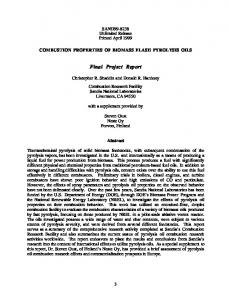
Fig. 2. The effects of a few common filter types on a swept-frequency input signal [2] In the example above, an input signal of constant amplitude and increasing frequency’s signal is passed through a filter. As the signal moves out of the pass band, the filter starts to attenuate the signal. Take note that a signal’s transition from a pass band to stop band or vice versa is a gradual process where amplitude decreases smoothly. Although this transition can be made instantaneously sharp or close enough by increasing orders of a filter as higher order results in the filter reaching its steady state faster or in other words quickly remove the stop band frequencies. 6

iii.

FILTERS

a. Active and Passive filters

Filters are divided into two distinct types: active filters and passive filters. Active filters contain components like an operational amplifier or a transistor which provide gain (beside the input signal) thereby increasing the output signal’s strength unlike passive filters which contain no such elements in its circuit, just the passive elements such as resistors, capacitors and/or inductors.Due to this factor, the signals passing through a passive filter, suffers from attenuation and hence the gain is always less than unity. Active filters draw their power from an external power source and use it to amplify or boost up their signal providing a voltage gain of unity. Passive filters may consist of inductors which allow its use in high frequency signals hence providing frequency selectivity unlike active filters which never have inductors in its circuit. Typically the frequency range of an active filter is dependent on the bandwidth of the amplifier. Still, active filters give better performance and easier to design, very good accuracy with a steep roll-off and low noise with an appropriate circuit design. Due to high input impedance of active pass filter prevents excessive loading on the filters while its low output impedance avoids affecting the filter’s cut-off frequency point due to changes in the impedance of load. Hence properties of active pass filters are relatively more stable than passive low pass filters under the effect of changing load impedances.

b. Low pass filters Our primary focus of this project proposal is on comparison between the responses of both active and passive second order low pass filters’ responses. A simple passive RC low pass filter can be made by connecting a resistor and a capacitor in series and the output Voutis measured across the capacitor only (across the resistor for high pass filter). This filter is of first order which generally means it has only a single pole as there is only a single reactive component, i.e. the capacitor.

7

Fig. 3. RC Low Pass Filter Circuit (Passive filter) [3] As we may know that the reactance of a capacitor is inversely proportional to frequency of an input signal while the value of a resistor remains constant. So at lower frequencies the reactance (Xc) will be very large compared to the resistance of the resistor, R. So the voltage potential, Vout will be far greater than the voltage drop across the capacitor Vr. At higher frequencies, the reverse is true where Vout is significantly lower than Vr.

Fig. 4. An active first order low pass filter [4] Its principle operation and frequency response is exactly the same as discussed previously for passive filters, the only way it differs is in the use of an op-amp for amplification and gain control. The simplest way to build an active low pass filter is to connect inverting or noninverting amplifier as shown in Fig. 4. The simple first-order active low pass filter consists of RC filter stage providing low frequency path to the input of a non-inverting operational amplifier. The amplifier is configured as a voltage-buffer providing a DC gain of one or unity unlike the passive filter which has a DC gain less than that of unity.

8

Figure 5: Active Low Pass filter with Amplification [5] The frequency response of circuit in Figure 5 is exactly the same as that of passive filter with just the difference in increased pass gain, Af of the amplifier. For a non-inverting amplifier circuit, the value of the voltage gain is given as a function of the feedback resistor R2 divided by the corresponding input resistor R1 :

𝐷𝐶𝐺𝑎𝑖𝑛 = [1 +

𝑅2 ] 𝑅1

where, R1 = resistor connected to ground R2 = resistor in feedback There the gain of first order low pass filter is

𝑉𝑜𝑙𝑡𝑎𝑔𝑒𝐺𝑎𝑖𝑛, (𝐴𝑣 ) =

𝑉𝑜𝑢𝑡 = 𝑉𝑖𝑛

𝐴𝐹 𝑓

√1 + ( 𝑓 ) 2 𝑐

where, Af = the pass band gain of the filter f = input signal’s frequency in Hertz, (Hz) fc = the cut-off frequency in hertz, (Hz)

9

Fig. 6. Passive second-order low pass filter [6]

Fig. 7. Active second-order low pass filter [7]

iv.

APPLICATIONS

In Bangladesh, low pass filters are mainly used in radio centers and airport signal receiving center. Radars are to receive the radio waves and filter the frequencies as signal is sent from the sender or other source. Especially the active low pass filter is used to avoid the extra unnecessary frequencies and noises. But in different devices such as speakers, micro phones, base sound boxes and acoustics in recording room low pass filters are also highly used in Bangladesh. So controlled active low pass filter having shorter settling time will be very effective in these perspectives of developing radio centers and airport signal receiving centers of Bangladesh.

10

v.

MATHEMATICAL MODELS & TRANSFER FUNCTIONS

Mathematical Model of Passive Filter: (Refer Appendix A for all derivations) 𝑉𝑥 −𝑉𝑖𝑛 𝑅1

Vx −Vo

+

+ sC1 Vx = 0

R2

where, Vx = voltage across node Vin = applied voltage Vo = output voltage R1 = resistance R2 = resistance C1 = capacitance The mathematical model is derived from Fig. 6.using Ohm’s law, KCL and KVL. We then convert this model to an interpretation on which control engineering techniques can be applied which is the transfer function. Then further we can analyze the transfer function to evaluate the system’s performance. Transfer function of passive filter: 1

H(s) =

s 2 + s (R

1

1 C1

R1 R2 C1 C2 1 1

+R

2 C1

+R

2 C2

)+R

1

1 R2 C1 C2

Mathematical model of active filter:

𝑉𝑖𝑛 − 𝑉1 V1 V1 − Vo = + 𝑅1 R 2 + Z2 Z1 where, s=jω and Zn= 1/jωCn Transfer function of active filter:

11

1

H(s) =

𝑠² + 𝑠 (𝑅

𝑅1 𝑅2 𝐶1 𝐶2 1 1

2 𝐶1

vi.

+𝑅

1 𝐶1

)+𝑅

1

1 𝑅2 𝐶1 𝐶2

ANALYSIS:

The transfer functions of passive and active low pass filters are used in MATLAB to get the pole-zero maps and step response curves to analyze the system of the low pass filter by poles’ position on real axis which determines whether the system is stable or not and the step response shows how steady the response of the system when step input response is applied. Also from the step response curve we can predict what should be done in order to stabilize the system or improve its performance.

a. Pole-zero map Pole-Zero Map for passive low pass filter Imaginary Axis (seconds-1)

1

0.5

0

-0.5

-1 -3000

-2500

-2000Real Axis-1500 (seconds-1) -1000

-500

0

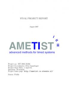
Fig. 8. Passive Low Pass Filter Pole-Zero Map In Fig. 8, both the poles are on the left hand side of the imaginary axis i.e. at around -2600 and 400 on the real axis. The poles’ positions confirm that the passive low pass filter is stable as there is not a single pole on the right hand side of the imaginary axis.

12

Pole-Zero Map for active low pass filter Imaginary Axis (seconds-1)

1

0.5

0

-0.5

-1 -1200

-1000

-800Real Axis-600 (seconds-1) -400

-200

0

Fig.9. Active Low Pass Filter Pole-Zero Map In Fig. 9, both the poles are on the left hand side of the imaginary axis i.e. double poles on -1000 on the real axis. The poles’ positions confirm that the active low pass filter is also stable as there is not a single pole on the right hand side of the imaginary axis.

b. Step Response Step Response for passive low pass filter 1

Amplitude

0.8 0.6 0.4 0.2 0 0

0.005

0.01 0.015 Time (seconds)

0.02

0.025

Fig. 10. Passive Low Pass Filter step response curve. The following we can evaluate from Fig.10. Settling time: 0.015 seconds Rise time: 0.01 seconds Overshoot: None Steady-state error: None

13

Step Response for active low pass filter 1

Amplitude

0.8 0.6 0.4 0.2 0 0

0.002

0.004 Time (seconds) 0.006

0.008

0.01

0.012

Fig. 11. Active Low Pass Filter step response curve. The following we can evaluate from Fig.11. Settling time: 0.008 seconds Rise time: 0.006 seconds Overshoot: None Steady-state error: None From Fig. 8 to Fig. 11. we can conclude that both active and passive low pass filters are stable. From the step response curves the speed of the both low pass filters to reach the settling time is measured and those are 0.015 seconds for passive and 0.008 seconds for active low pass filter which confirms that the active low pass filter is faster than the passive low pass filter. But we can make active low pass filter system muchfaster than the one shown in Fig. 11.Both the systems are critically damped and they do not have any overshoot and steady state error. Also from the circuit diagram for active and passive low pass filter it is proved that the passive low pass filter is an open loop system (no feedback) and active low pass filter is a closed loop system (with feedback mechanism).

vii.

PID CONTROLLER

A PID (proportional-integral-derivative) controller is a controller used to control loop feedback systems only. A PID controller repeatedly calculates the difference between a desired set point and a measured process variable and that difference is specifically knows as the error e(t). A PID controller has three parameters proportional, integral and derivative and their respective coefficients are denoted by Kp, Ki and Kd. In order to be able to explain its functionality better, we can consider a unity feedback system

14

Fig. 12. Unity feedback system [12] The total output to the above system including the controller and the plant in time-domain as follows:

𝑢(𝑡) = 𝐾𝑝 𝑒(𝑡) + 𝐾𝑖 ∫ 𝑒(𝑡)𝑑𝑡 + 𝐾𝑝

𝑑𝑒 𝑑𝑡

The variables on the Fig.12. is as follows where e is the difference between the output y and the input r regarded as the error of the measured output value. The controller calculates both the derivative and the integral of this error signal when initially error signal is forwarded to the controller. The output of the controller u is equivalent to the proportional gain Kp times the error plus integral gain Ki times the integral of the error which is then further added to the derivative gain Kd times the derivative of the error signal. The control signal u is then fed to the plant to yield an output y which is fed back to the system to be compared with the desired value and to find the new error signal. The controller takes in the new error signal and the cycle repeats. The transfer function of a PID controller is evaluated using Laplace transform on Eq. in order to obtain a form on which controlling engineering techniques can be applied.

𝐾𝑑 𝑠 2 + 𝐾𝑝 𝑠 + 𝐾𝑖 𝐾𝑖 𝐾𝑝 + + 𝐾𝑑 𝑠 = 𝑠 𝑠

The Distinguishing Properties of P, I, and D Controllers The effects of each controller parameters, Kp, Kd and Ki is summarized below in the table

15

CL RESPONSE RISE TIME OVERSHOOT SETTLING TIME S-S ERROR Kp

Decrease

Increase

Small Change

Decrease

Ki

Decrease

Increase

Increase

Eliminate

Kd

Small Change Decrease

Decrease

No Change

Care should be taken that each parameters affect one another when two or more are used together so this table is just used for reference.

P Controlled Step Response: Active low pass filter 0.8

Amplitude

0.6

0.4

0.2

0 0

0.002

0.004 0.006 Time (seconds) Fig. 12. P controlled step response curve for Active low pass filter.

0.008

0.01

The above step response curve is after applying only proportional gain controlof valueKp=3. The graph is far away from the desired amplitude which is 1 and have huge steady state error. The system is then said to be overdamped. So, only P controller is not able to make this system faster without error and less overshoot.

16

1

PD Controlled Step Response - Active low pass filter

Amplitude

0.8 0.6 0.4 0.2 0 0

0.002


0.008

0.01

Fig.13. PD controlled step response curve for Active low pass filter after applying Kp=3 & Kd=10. After applying both proportional and derivative gain control with Kp =3 and Kd = 10, this above step response curve is stable again and with reduced settling time, no overshoot and no steady state error.So, PD controller is able to control this system perfectly by making it faster than before from initial 0.008 seconds settling time to 0.001 seconds reaching our desired value of amplitude = 1.

1

PID Controlled Step Response - Active low pass filter

Amplitude

0.8 0.6 0.4 0.2 0 0

0.002


0.008

0.01

17

Fig. 13. PID controlled step response curve for Active low pass filter after applying Kp = 3, Ki = 2 & Kd = 10. Here in this step response curve PID controller is used where Kp = 3,Ki = 2 and Kd = 2. The step response is stable and the settling time is also 0.001 seconds. Observing Fig. 12. And Fig 13, there is no observable change in the steady state responses. So we can then come to this conclusion that addition of the integral gain makes no difference since responses of both PID and PD controlled graphs are identical. In order to reduce the complexity of the system thereby the cost of the system we opt for

viii. DISCUSSION Among the two types of filters- the passive and the active- only active filter can be controlled due to the presence of feedback .We need a closed loop feedback system in order to control or manipulate the system by using a PID controller. Active low pass filter is faster than passive low pass filter and can be made faster than it already is. The system is already stable here. No overshoot and no steady state errors were seen in the initial step response curves. But while controlling and doing trial and error we got some drastic responses due to the effect of control parameters used. First applying Kp we noticed the system is overdamped with huge steady state error.. Secondly, applying both Kp and Kd we saw much improvement in the step response of the system. The system had the settling time of 0.001s with no overshoot. With the aim to improve the system further we applied all the three control parameters,and obtained the same response as compared to the second case. So we choose PD controller over PID controller to control the low pass active filter as manufacturing PD would involve lesser complexity (eg. less voltage required) and hence would be more economical than PID..

ix.

CONCLUSION

Summing all up, we can conclude that active low pass filter is faster than passive low pass filter of which its performance can be further improved by using a PID controller achieving a settling time from 0.008 seconds to 0.001 seconds with no steady state error and overshoot. Only PD controller is used over PID with very small co-efficient values of Kp and Kd.

18

x.

REFERENCES

[1] Ideal Filter Response curves [Digital image]. (n.d.). Retrieved April 10, 2016, from http://www.electronics-tutorials.ws/filter/filter_5.html [2] [The effects of a few common filter types on a swept-frequency input signal]. (n.d.). Retrieved April 10, 2016, from http://www.sensorsmag.com/sensors/electric-magnetic/anintroduction-analog-filters-1023 [3] RC Low Pass Filter Circuit [Digital image]. (n.d.). Retrieved April 10, 2016, from http://www.electronics-tutorials.ws/filter/filter2.html [4] Active first order low pass filter [Digital image]. (n.d.). Retrieved April 10, 2016, from http://www.electronics-tutorials.ws/filter/filter_5.html [5] Active Low Pass filter with Amplification [Digital image]. (n.d.). Retrieved April 10, 2016, from http://www.electronics-tutorials.ws/filter/filter_5.html [6] Passive second-order low pass filter [Digital image]. (n.d.). Retrieved April 10, 2016, from http://electronics.stackexchange.com/questions/152159/deriving-2nd-order-passive-low-passfilter-cutoff-frequency [7] Active second-order low pass filter [Digital image]. (n.d.). Retrieved April 10, 2016, from https://en.wikipedia.org/wiki/Linear_filter [8] N. (n.d.). Difference Between Active and Passive Filters. Retrieved March 4, 2016, from http://pediaa.com/difference-between-active-and-passive-filters-2/ [9] Low Pass Filter - Passive RC Filter Tutorial. (n.d.). Retrieved March 04, 2016, from http://www.electronics-tutorials.ws/filter/filter_2.html [10] Active Low Pass Filter - Op-amp Low Pass Filter. (n.d.). Retrieved March 04, 2016, from http://www.electronics-tutorials.ws/filter/filter_5.html [11] Control Tutorials for MATLAB and Simulink. (n.d.). Retrieved April 10, 2016, from http://ctms.engin.umich.edu/CTMS/index.php?example=Introduction [12] Unity feedback system [Digital image]. (n.d.). Retrieved April 10, 2016, from http://ctms.engin.umich.edu/CTMS/index.php?example=Introduction§ion=ControlPID

19

xi.

APPENDIX A : Derivations of Mathematical models and Transfer functions

20

21

22

23

24

25

26

27

xii.

APPENDIX B : MATLAB codes

Contents 

Transfer function (Passive low pass filter)



Poles



Pole-zero plot



step-response



Transfer function (Active low pass filter)



Poles



Pole-Zero plot



step-response



P Controller (Active low pass filter)



PD Controller (Active low pass filter)



PID Controller (Active low pass filter)

% Group Name- NINJA TURTLES % 11th April 2016

Transfer function (Passive low pass filter) num = [1000000]; den = [1 3000 1000000]; sys1 = tf(num,den)

sys1 =

1e06 ------------------s^2 + 3000 s + 1e06

28

Continuous-time transfer function.

Poles pole(sys1)

ans =

1.0e+03 *

-2.6180 -0.3820

Pole-zero plot pzmap(sys1)

29

step-response step(sys1)

30

Transfer function (Active low pass filter) num = [1000000]; den = [1 2000 1000000]; sys2 = tf(num,den)

sys2 =

1e06 ------------------s^2 + 2000 s + 1e06


Poles pole(sys2)

ans =

1.0e+03 *

-1.0000 -1.0000

31

Pole-Zero plot pzmap(sys2)

step-response step(sys2)

32

P Controller (Active low pass filter) Kp = 3; Kd = 0; Ki= 0; C = pid(Kp,0,0); num = [1000000]; den = [1 2000 1000000]; sys_21 = tf(num,den)

T = feedback(C*sys_21,1);

t = 0:0.001:0.01;

33

step(T,t) gridon

sys_21 =

1e06 ------------------s^2 + 2000 s + 1e06


PD Controller (Active low pass filter) Kp = 3; Kd = 10;

34

Ki= 0; C = pid(Kp,0,Kd); num = [1000000]; den = [1 2000 1000000]; sys_22 = tf(num,den)


t = 0:0.001:0.01; step(T,t) gridon

sys_22 =

1e06 ------------------s^2 + 2000 s + 1e06


35

PID Controller (Active low pass filter) Kp = 3; Kd = 10; Ki= 2; C = pid(Kp,Ki,Kd); num = [1000000]; den = [1 2000 1000000]; sys_23 = tf(num,den)


t = 0:0.001:0.01;

36

step(T,t) gridon

sys_23 =

1e06 ------------------s^2 + 2000 s + 1e06


Published with MATLAB® R2014a

37