Memorandum series to issue informal scientific and technical publications when ...... Predicted relative density estimates for Dall's porpoise (top) and northern ...
T
M
EN
T OF CO
M M
CE
DEP
ER
AR
NOAA Technical Memorandum NMFS
E
E
D
R
IT
IC
UN
A
MAY 2009
ST
AT E S O F A
M
PREDICTIVE MODELING OF CETACEAN DENSITIES IN THE EASTERN PACIFIC OCEAN
Jay Barlow Megan C. Ferguson Elizabeth A. Becker Jessica V. Redfern Karin A. Forney Ignacio L. Vilchis Paul C. Fiedler Tim Gerrodette Lisa T. Ballance
NOAA-TM-NMFS-SWFSC-444
U.S. DEPARTMENT OF COMMERCE National Oceanic and Atmospheric Administration National Marine Fisheries Service Southwest Fisheries Science Center
The National Oceanic and Atmospheric Administration (NOAA), organized in 1970, has evolved into an agency that establishes national policies and manages and conserves our oceanic, coastal, and atmospheric resources. An organizational element within NOAA, the Office of Fisheries is responsible for fisheries policy and the direction of the National Marine Fisheries Service (NMFS). In addition to its formal publications, the NMFS uses the NOAA Technical Memorandum series to issue informal scientific and technical publications when complete formal review and editorial processing are not appropriate or feasible. Documents within this series, however, reflect sound professional work and may be referenced in the formal scientific and technical literature.
NOAA Technical Memorandum NMFS IC
This TM series is used for documentation and timely communication of preliminary results, interim reports, or special purpose information. The TMs have not received complete formal review, editorial control, or detailed editing.
.
R CE
EA N NATIO NAL OC
S U.
DE
D ATMOSPHER
TRATION NI S MI AD
IC
AN
ME PA RTM OM ENT OF C
MAY 2008
PREDICTIVE MODELING OF CETACEAN DENSITIES IN THE EASTERN PACIFIC OCEAN
Jay Barlow, Megan C. Ferguson, Elizabeth A. Becker, Jessica V. Redfern, Karin A. Forney, Ignacio L. Vilchis, Paul C. Fiedler, Tim Gerrodette, and Lisa T. Ballance
National Oceanic & Atmospheric Administration National Marine Fisheries Service Southwest Fisheries Science Center 3333 Torrey Pines Court La Jolla, California, USA 92037
NOAA-TM-NMFS-SWFSC-444
U.S. DEPARTMENT OF COMMERCE Gary F. Locke, Secretary National Oceanic and Atmospheric Administration Jane Lubchenco, Undersecretary for Oceans and Atmosphere National Marine Fisheries Service James W. Balsiger, Acting Assistant Administrator for Fisheries
Final Technical Report: PREDICTIVE MODELING OF CETACEAN DENSITIES IN THE EASTERN PACIFIC OCEAN (SI-1391) Jay Barlow Megan C. Ferguson Elizabeth A. Becker Jessica V. Redfern Karin A. Forney Ignacio L. Vilchis Paul C. Fiedler Tim Gerrodette Lisa T. Ballance
May 2009
Prepared for the U.S. Department of Defense, Strategic Environmental Research and Development Program By the U.S. Department of Commerce, NOAA Fisheries, Southwest Fisheries Science Center. Approved for public release; distribution is unlimited
i
This report was prepared under contract to the Department of Defense Strategic Environmental Research and Development Program (SERDP). The publication of this report does not indicate endorsement by the Department of Defense, nor should the contents be construed as reflecting the official policy or position of the Department of Defense. Reference herein to any specific commercial product, process, or service by trade name, trademark, manufacturer, or otherwise, does not necessarily constitute or imply its endorsement, recommendation, or favoring by the Department of Defense.
ii
iii
Table of Contents Acronyms and Abbreviations .................................................................................................. xiii Acknowledgements ..................................................................................................................xiv Executive Summary .................................................................................................................. xv 1.0 Objective ...............................................................................................................................1 2.0 Background ...........................................................................................................................2 3.0 Materials and Methods ..........................................................................................................5 3.1 Data Sources ......................................................................................................................5 3.1.1 Marine Mammal Surveys ............................................................................................5 3.1.2 In situ Oceanographic Measurements ..........................................................................8 3.1.3 Remotely Sensed Oceanographic Measurements .........................................................8 3.1.4 Water Depth and Bottom Slope ...................................................................................9 3.1.5 Mid-trophic Sampling with Net Tows and Acoustic Backscatter ................................ 10 3.2 Oceanographic Data Interpolation .................................................................................... 12 3.3 Modeling Framework....................................................................................................... 15 3.3.1 GLM and GAM Models ............................................................................................ 15 3.3.2 CART Tree-based Models ......................................................................................... 19 3.4 Model Scale: Resolution and Extent ................................................................................. 19 3.5 Model Selection ............................................................................................................... 20 3.5.1 California Current Ecosystem Models ....................................................................... 21 3.5.2 Eastern Tropical Pacific Models ................................................................................ 27 3.5.3 Line-transect densities for unmodeled species............................................................ 31 3.6 Variance Estimation ......................................................................................................... 35 3.7 Inclusion of Prey Indices from Net Tow and Acoustic Backscatter Data in Models .......... 36 3.8 Seasonality ...................................................................................................................... 37 3.9 Model Output and Visualization Software ........................................................................ 39 4.0 Results and Accomplishments ............................................................................................. 41 4.1 Oceanographic Data Interpolation .................................................................................... 41 iv
4.1.1 Comparison of Interpolation Methods........................................................................ 41 4.1.2 Yearly interpolated fields of habitat variables ............................................................ 41 4.2 Modeling Framework : GLM and GAM........................................................................... 48 4.2.1 Comparisons of GAM Algorithms ............................................................................. 48 4.2.2 Encounter Rate Models ............................................................................................. 49 4.2.3 Group Size Models .................................................................................................... 49 4.2.4 Conclusions Regardings Modeling Approaches ......................................................... 50 4.3 Model Scale: Resolution and Extent ................................................................................. 55 4.3.1 Resolution ................................................................................................................. 55 4.3.2 Extent ........................................................................................................................ 57 4.4 Variance Estimation ......................................................................................................... 61 4.5 Inclusion of Prey Indices in Habitat Models ..................................................................... 63 4.6 Seasonal Predictive Ability of Models ........................................................................... 72 4.6.1 Model performance ................................................................................................... 72 4.6.2 Seasonal Predictive Ability ........................................................................................ 73 4.7 Model Validation ............................................................................................................. 73 4.7.1 California Current Ecosystem Models ....................................................................... 73 4.7.2 Eastern Tropical Pacific Models ................................................................................ 75 4.8 Final Models for the California Current Ecosystem .......................................................... 80 4.9 Final Models for the Eastern Tropical Pacific................................................................... 85 4.10 Model Output and Visualization Software ...................................................................... 90 5.0 Conclusion .......................................................................................................................... 92 6.0 Transition Plan .................................................................................................................... 94 7.0 References ........................................................................................................................... 97 Appendix A: Detailed Model Results for the California Current Ecosystem ........................... 104 Appendix B: Detailed Model Results for the Eastern Tropical Pacific .................................... 133 Appendix C: List of Technical Publications ............................................................................ 201 v
C.1 Journal Publications ...................................................................................................... 201 C.2 PhD Dissertations .......................................................................................................... 201 C.3 Technical Reports ......................................................................................................... 202 C.4 Conference Proceedings ................................................................................................ 202 C.5 Related Publications ...................................................................................................... 203
vi
List of Figures Figure 1. Transects (green lines) surveyed for cetacean abundance in the California Current Ecosystem by the SWFSC 1991-2005 CCE .................................................................................6 Figure 2. Transects (green lines) surveyed for cetaceans in the ETP by the SWFSC 1986-2006 ...................................................................................................................................................6 Figure 3. Completed transects for the winter/spring aerial line-transect surveys conducted off California in March-April 1991 and February-April 1992 ...........................................................7 Figure 4. Geographical distribution of manta and bongo tow stations ...................................... 10 Figure 5. Mean volume backscattering strength, Svmean, in six hour segments along the a) 2003 and b) 2006 transects surveyed by the NOAA ship David Starr Jordan in the eastern tropical Pacific, and c) 2001 and d) 2005 transects surveyed by the NOAA ships David Starr Jordan and McArthur in the California Current ecosystem .......................................................................... 11 Figure 6. Geographic strata used for the CCE spatial predictions .............................................. 25 Figure 7. Geographic strata used for ETP model selection and validation ................................. 29 Figure 8. Stratum numbers for ETP line-transect density estimates for coastal spotted dolphin, killer whale, and sperm whale (from Ferguson and Barlow 2003) ............................................. 32 Figure 9. Thermocline depth (m) observed in 2006 interpolated using five methods; the ±sd of residuals are shown for both jackknife procedures (single, daily). The map on the lower right is an August-October climatology from Fiedler and Talley (2006) ............................................... 42 Figure 10. 2006 thermocline depth residuals (observed value – interpolated value, m) for interpolation by inverse distance squared and kriging, from jackknifing of observations singly and daily (by ship-day) ............................................................................................................. 42 Figure 11. Surface chlorophyll (mg m-3) observed in 2005 interpolated using five methods; the ±sd of residuals are shown for both jackknife procedures (single, daily) ................................... 43 Figure 12. Yearly grids of ETP thermocline depth .................................................................... 45 Figure 13. Yearly grids of CCE surface chlorophyll ................................................................. 46 Figure 14. Yearly grids of CCE sea surface temperature ........................................................... 47 Figure 15. The transect lines used to collect dolphin and oceanographic data in the California Current ecosystem are shown for 1991, 1993, 1996, and 2001 ................................................... 56 Figure 16. Densities were predicted at small, intermediate, and large resolutions and interpolated in a 5 km x 5 km grid using negative exponential distance weighting to produce the maps shown ................................................................................................................................................. 58 Figure 17. Encounter rate models built at a 60 km resolution for striped dolphin to explore the effect of extent .......................................................................................................................... 59 vii
Figure 18. Encounter rate models built at a 60 km resolution for short-beaked common dolphin to explore the effect of extent .................................................................................................... 60 Figure 19. Predicted average density (AveDens), standard error (SE(Dens)), and upper and lower lognormal 90% confidence limits(Lo90% and Hi90%) based on the final complex ETP encounter rate (53.4 effective degrees of freedom) and group size (17.9 effective degrees of freedom) models for striped dolphins ........................................................................................ 62 Figure 20. Predicted average density (AveDens), standard error (SE(Dens)), and upper and lower lognormal 90% confidence limits(Lo90% and Hi90%) based on a simple ETP encounter rate (22.5 effective degrees of freedom) and group size (12.6 effective degrees of freedom) models for striped dolphins ....................................................................................................... 62 Figure 21. Predicted average density (AveDens), standard error (SE(Dens)), and upper and lower lognormal 90% confidence limits (Lo90% and Hi90%) based on models for: (A) shortbeaked common dolphin and (B) Dall’s porpoise ...................................................................... 63 Figure 22. Maps of the predicted number of sightings in the ETP for models that include only oceanographic data or a combination of oceanographic, net-tow, and acoustic backscatter data ................................................................................................................................................. 67 Figure 23. Maps of the predicted number of sightings in the CCE for models that include only oceanographic data, only net-tow data, or a combination of oceanographic, net-tow, and acoustic backscatter data ......................................................................................................................... 71 Figure 24. Predicted relative density estimates for Dall’s porpoise (top) and northern right whale dolphin (bottom): (A) summer predictions based on the summer shipboard models and (B) winter predictions based on the summer shipboard models ........................................................ 74 Figure 25. Sample 2005 validation plots for models developed using 1991-2001 survey data. Left: northern right whale dolphin, Center: Risso's dolphin, Right: Baird's beaked whale .......... 76 Figure 26. Predicted yearly and averaged densities for Dall’s porpoise based on the final CCE models ...................................................................................................................................... 85 Figure 27. Average density (AveDens), standard error (SE(Dens)), and upper and lower lognormal 90% confidence limits(Lo90% and Hi90%) for Dall’s porpoise ................................ 86 Figure 28. Screenshot from the SDSS development website of blue whale sightings and predicted density in the eastern tropical Pacific Ocean............................................................... 91 Appendix A, Figure A-1. Predicted yearly and averaged densities based on the final CCE models for: (a) striped dolphin (Stenella coeruleoalba), (b) short-beaked common dolphin (Delphinus delphis), (c) Risso’s dolphin (Grampus griseus), (d) Pacific white-sided dolphin (Lagenorhynchus obliquidens), (e) northern right whale dolphin (Lissodelphis borealis), (f) Dall’s porpoise (Phocoenoides dalli), (g) sperm whale (Physeter macrocephalus), (h) fin whale (Balaenoptera physalus), (i) blue whale (Balaenoptera musculus), (j) humpback whale viii
(Megaptera novaeangliae), (k) Baird’s beaked whale (Berardius bairdii), and (l) small beaked whales (Ziphius and Mesoplodon) .......................................................................................... 107 Appendix A, Figure A-2. Predicted average density (AveDens), standard error (SE(Dens), and upper and lower lognormal 90% confidence limits(Lo90% and Hi90%) based on the final CCE models for: (a) striped dolphin (Stenella coeruleoalba), (b) short-beaked common dolphin (Delphinus delphis), (c) Risso’s dolphin (Grampus griseus), (d) Pacific white-sided dolphin (Lagenorhynchus obliquidens), (e) northern right whale dolphin (Lissodelphis borealis), (f) Dall’s porpoise (Phocoenoides dalli), (g) sperm whale (Physeter macrocephalus), (h) fin whale (Balaenoptera physalus), (i) blue whale (Balaenoptera musculus), (j) humpback whale (Megaptera novaeangliae), (k) Baird’s beaked whale (Berardius bairdii), and (l) small beaked whales (Ziphius and Mesoplodon) .......................................................................................... 120 Appendix B, Figure B-1. Predicted yearly and averaged densities (animals per km2) based on the final ETP models for: (a) offshore spotted dolphin (Stenella attenuata), (b) eastern spinner dolphin (Stenella longirostris orientalis), (c) whitebelly spinner dolphin (Stenella longirostris longirostris), (d) striped dolphin (Stenella coeruleoalba), (e) rough-toothed dolphin (Steno bredanensis), (f) short-beaked common dolphin (Delphinus delphis), (g) bottlenose dolphin (Tursiops truncatus), (h) Risso’s dolphin (Grampus griseus), (i) Cuvier’s beaked whale (Ziphius cavirostris), (j) blue whale (Balaenoptera musculus), (k) Bryde’s whale (Balaenoptera edeni), (l) short-finned pilot whale (Globicephala macrorhynchus), (m) dwarf sperm whale (Kogia sima), (n) Mesoplodon beaked whales (including Mesoplodon spp., Mesoplodon densirostris, and Mesoplodon peruvianus), and (o) small beaked whales (Mesoplodon beaked whales plus “unidentified beaked whale”) ................................................................................................. 162 Appendix B, Figure B-2. Predicted average density (AveDens), standard error (SE(Dens)), and lower and upper lognormal 90% confidence limits(Lo90% and Hi90%) based on the final ETP models for: (a) offshore spotted dolphin (Stenella attenuata), (b) eastern spinner dolphin (Stenella longirostris orientalis), (c) whitebelly spinner dolphin (Stenella longirostris longirostris), (d) striped dolphin (Stenella coeruleoalba), (e) rough-toothed dolphin (Steno bredanensis), (f) shortbeaked common dolphin (Delphinus delphis), (g) bottlenose dolphin (Tursiops truncatus), (h) Risso’s dolphin (Grampus griseus), (i) Cuvier’s beaked whale (Ziphius cavirostris), (j) blue whale (Balaenoptera musculus), (k) Bryde’s whale (Balaenoptera edeni), (l) short-finned pilot whale (Globicephala macrorhynchus), (m) dwarf sperm whale (Kogia sima), (n) Mesoplodon beaked whales (including Mesoplodon spp., Mesoplodon densirostris, and Mesoplodon peruvianus), and (o) small beaked whales (Mesoplodon beaked whales plus “unidentified beaked whale”) ................................................................................................. 192
ix
List of Tables Table 1. Summary of satellite-derived sea surface temperature (SST) and CV(SST) spatial resolutions selected for ten California Current Ecosystem species ...............................................9 Table 2. Variogram model results ............................................................................................. 14 Table 3. Range of annual sample sizes (N) and search parameters for kriging of grid points ..... 15 Table 4. Summary of the weighted effective strip width (ESW = 1/ f(0)) and g(0) estimates used to calculate predicted densities for the CCE ............................................................................... 24 Table 5. Total number of sightings used to build, validate, and parameterize the final models for the ETP ..................................................................................................................................... 28 Table 6. Geographically stratified estimates of abundance (N), density (D), coefficient of variation (CV), and lognormal 90% confidence intervals of density for unmodeled cetacean species in the California Current Ecosystem .............................................................................. 33 Table 7. Geographically stratified estimates of abundance (N), density (D), coefficient of variation (CV), and lognormal 90% confidence intervals of density for three ETP cetacean species ...................................................................................................................................... 34 Table 8. Geographically stratified estimates of abundance (N), density (D), coefficient of variation (CV), and lognormal 90% confidence intervals for unmodeled cetacean species within EEZ waters of the Hawaiian Islands .......................................................................................... 34 Table 9. Number of segments containing a sighting and the total number of sightings used to build mid-trophic models in the ETP and CCE .......................................................................... 37 Table 10. Comparison of the simple and complex encounter rate GAMs for the ETP ................ 51 Table 11. Comparison of the simple and complex group size GAMs for the ETP ...................... 53 Table 12. Number of encounters for the four species and six spatial resolutions considered in our California Current ecosystem analyses ...................................................................................... 56 Table 13. Variables selected for models built using oceanographic, net-tow, acoustic backscatter, and a combination of all data to determine whether indices of mid-trophic species improve cetacean-habitat models ............................................................................................................ 66 Table 14. Starting and final AIC values for models of the number of sightings of each species built using oceanographic, net-tow, acoustic backscatter, or a combination of all data ............... 68 Table 15. The explained deviance for the models of the number of sightings of each species built using oceanographic, net-tow, acoustic backscatter, or a combination of all data ....................... 68 Table 16. Ratios of observed to predicted number of sightings in the ETP (SE = Standard Error) ................................................................................................................................................. 69 Table 17. Ratios of observed to predicted number of sightings in the CCE................................ 70 x
Table 18. Spatial and temporal estimates of the number of animals observed in each geographic stratum, calculated using line-transect methods (LT) and predicted based on results from the 1991-2001 CCE models (Pred) ................................................................................................. 77 Table 19. Data type (remotely sensed [RS] or combined remotely sensed and in situ [CB]) and number of sightings used to build, validate, and parameterize the final models for the CCE ...... 81 Table 20. Abundance (number of animals) predicted based on results from the final CCE models and calculated using line-transect methods (Barlow 2003) ........................................................ 82 Table 21. Predictor variables included in the final encounter rate (ER) and group size (GS) GAMs for the CCE ................................................................................................................... 83 Table 22. Proportion of deviance explained (Expl. Dev.) and average squared prediction error (ASPE) for the final encounter rate (ER) and group size (GS) models for the CCE .................... 84 Table 23. Effective degrees of freedom for each predictor variable included in the final encounter rate GAMs for the ETP ............................................................................................. 88 Table 24. Effective degrees of freedom for each predictor variable included in the final group size GAMs for the ETP ............................................................................................................. 89 Appendix A, Table A-1. Spatial and temporal estimates of the number of animals observed in each geographic stratum, calculated using line-transect methods (LT) and predicted based on results from the final CCE models (Pred) ............................................................................... 104 Appendix B, Table B-1. Summary of model validation statistics for final offshore spotted dolphin density models in the ETP built on 1998-2003 SWFSC survey data and tested on 2006 SWFSC survey data ................................................................................................................ 133 Appendix B, Table B-2. Summary of model validation statistics for final eastern spinner dolphin density models in the ETP built on 1986-2003 SWFSC survey data and tested on 2006 SWFSC survey data ................................................................................................................ 134 Appendix B, Table B-3. Summary of model validation statistics for final whitebelly spinner dolphin density models in the ETP built on 1986-2003 SWFSC survey data and tested on 2006 SWFSC survey data ................................................................................................................ 136 Appendix B, Table B-4. Summary of model validation statistics for final striped dolphin density models in the ETP built on 1986-2003 SWFSC survey data and tested on 2006 SWFSC survey data ......................................................................................................................................... 138 Appendix B, Table B-5. Summary of model validation statistics for final rough-toothed dolphin density models in the ETP built on 1986-2003 SWFSC survey data and tested on 2006 SWFSC survey data .............................................................................................................................. 140
xi
Appendix B, Table B-6. Summary of model validation statistics for final short-beaked common dolphin density models in the ETP built on 1986-2003 SWFSC survey data and tested on 2006 SWFSC survey data ................................................................................................................ 142 Appendix B, Table B-7. Summary of model validation statistics for final bottlenose dolphin density models in the ETP built on 1986-2003 SWFSC survey data and tested on 2006 SWFSC survey data .............................................................................................................................. 144 Appendix B, Table B-8. Summary of model validation statistics for final Risso's dolphin density models in the ETP built on 1986-2003 SWFSC survey data and tested on 2006 SWFSC survey data ......................................................................................................................................... 146 Appendix B, Table B-9. Summary of model validation statistics for final Cuvier's beaked whale density models in the ETP built on 1986-2003 SWFSC survey data and tested on 2006 SWFSC survey data .............................................................................................................................. 148 Appendix B, Table B-10. Summary of model validation statistics for final blue whale density models in the ETP built on 1986-2003 SWFSC survey data and tested on 2006 SWFSC survey data ......................................................................................................................................... 150 Appendix B, Table B-11. Summary of model validation statistics for final Bryde's whale density models in the ETP built on 1986-2003 SWFSC survey data and tested on 2006 SWFSC survey data ......................................................................................................................................... 152 Appendix B, Table B-12. Summary of model validation statistics for final short-finned pilot whale density models in the ETP built on 1986-2003 SWFSC survey data and tested on 2006 SWFSC survey data ................................................................................................................ 154 Appendix B, Table B-13. Summary of model validation statistics for final dwarf sperm whale density models in the ETP built on 1986-2003 SWFSC survey data and tested on 2006 SWFSC survey data .............................................................................................................................. 156 Appendix B, Table B-14. Summary of model validation statistics for final Mesoplodon spp. density models in the ETP built on 1986-2003 SWFSC survey data and tested on 2006 SWFSC survey data .............................................................................................................................. 158 Appendix B, Table B-15. Summary of model validation statistics for final small beaked whale density models in the ETP built on 1986-2003 SWFSC survey data and tested on 2006 SWFSC survey data .............................................................................................................................. 160
xii
Acronyms and Abbreviations AIC ASPE CART CCA CCE CHL CTD CV CZCS EEZ ER ESW ETP GAM GCV GIS GLM MLD NASC NOAA SCORE SDSS SE SeaWIFS SERDP SSS SST SWFSC TD TS US XBT
Akaike Information Criterion Average Squared Prediction Error Classification and Regression Trees Canonical Correspondance Analysis California Current Ecosystem Surface Chlorophyll Conductivity, Temperature, and Depth measurment instrument Coefficient of Variation Coastal Zone Color Scanner Exclusive Economic Zone Encounter Rate Effective Strip Width Eastern Tropical Pacific Generalized Additive Model Generalized Cross Validation Geographic Information System Generalized Linear Model Mixed Layer Depth Nautical Area Scattering Coefficient National Oceanic and Atmospheric Administration Southern California Offshore Range Spatial Decision Support System software Standard Error Sea-viewing Wide Field-of-view Sensor Strategic Environmental Research and Development Program Sea Surface Salinity Sea Surface Temperature Southwest Fisheries Science Center Thermocline Depth Themocline Strength United States eXpendable BathyThermograph
xiii
Acknowledgements This project was funded by the Strategic Environmental Research and Development Program (SERDP) and by the National Oceanic and Atmospheric Administration (NOAA). Initial funding for cetacean habitat modeling was provided by the U.S. Navy’s Office of Naval Operations (N45), and we particularly thank Frank Stone and Ernie Young for their early support of this project. The marine mammal survey data and oceanographic data used to model cetacean density were collected by a large dedicated team at the Protected Resources Division of NOAA’s Southwest Fisheries Science Center. We particularly thank the cruise leaders, marine mammal observers, oceanographers, survey coordinators, ship’s crew, and officers who have worked hard over the past 20 years collecting the data that we use here. Physical oceanographic and midtropic data were collected and processed by Candice Hall, Melinda Kelley, Liz Zele, Bill Watson, Thomas J. Moore, Robert Holland, Valerie Andreassi, David Demer, Kerry Koptisky, George Watters, and Lindsey Peavey. We also thank Lucy Dunn, Barbara MacCall and Ioana Ionescu who collectively spent hundreds of hours sorting Bongo and Manta samples. Aerial survey efforts were lead by Jim Carretta. Steve Reilly and Robert Brownell were leaders of the Protected Resources Division during most of the surveys and were instrumental in providing the foundations upon which this project were based. We thank Dave Foley at SWFSC's Environmental Research Division for sharing his extensive knowledge of physical oceanography and providing code to automate the acquisition of remotely sensed data and Ray Smith at the University of California, Santa Barbara, for his thoughtful comments and insights on the results of our analyses. Our project benefitted greatly from our close collaboration with the SERDP Team at Duke University (SI-1390), particularly Ben Best, Andy Read, and Pat Halpin. We thank John Hall and an anonymous reviewer for their helpful suggestions on the draft final report.
xiv
Executive Summary The Navy and other users of the marine environment conduct many activities that can potentially harm marine mammals. Consequently, these entities are required to complete Environmental Assessments and Environmental Impact Statements to determine the likely impact of their activities. Specifically, those documents require an estimate of the number of animals that might be harmed or disturbed. A key element of this estimation is knowledge of cetacean (whale, dolphin, and porpoise) densities in specific areas where those activities will occur. Cetacean densities are typically estimated by line-transect surveys. Within United States Exclusive Economic Zone (US EEZ) waters and in the Eastern Tropical Pacific (ETP), most cetacean surveys have been conducted by the US National Marine Fisheries Service as part of their stock assessment research and typically result in estimates of cetacean densities in very large geographic strata (e.g., the entire US West Coast). Although estimates are sometimes available for smaller strata (e.g., the waters off southern California), these areas are still much larger than the operational areas where impacts may occur (e.g., the Navy’s Southern California Offshore Range (SCORE) off San Clemente Island). Stratification methods cannot provide accurate density estimates for small areas because sample size (i.e., the number of cetacean sightings) becomes limiting as areas become smaller. Recently, habitat modeling has been developed as a method to estimate cetacean densities. These models allow predictions of cetacean densities on a finer spatial scale than traditional line-transect analyses because cetacean densities are estimated as a continuous function of habitat variables (i.e., sea surface temperature, seafloor depth, distance from shore, prey density, etc.). Cetacean densities can then be predicted wherever these habitat variables can be measured or estimated, within the area that was modeled. We use data from 16 ship-based cetacean and ecosystem assessment surveys to develop habitat models to predict density for 15 cetacean species in the ETP and for 12 cetacean species in the California Current Ecosystem (CCE). All data were collected by NOAA’s Southwest Fisheries Science Center (SWFSC) from 1986-2006 using accepted, peer-reviewed survey methods. Data include over 17,000 sightings of cetacean groups on transects covering over 400,000 km. The expected number of groups seen per transect segment and the expected size of groups were modeled separately as functions of habitat variables. Model predictions were then used in standard line-transect formulae to estimate density for each transect segment for each survey year. Predicted densities for each year were smoothed with geospatial methods to obtain a continuous grid of density estimates for the surveyed area. These annual grids were then averaged to obtain a composite grid that represents our best estimates of cetacean density over the past 20 years in the ETP and the past 15 years in the CCE. Many methodological choices were required for every aspect of this modeling. In completing this project, we explored as many xv
of these choices as possible and used the choices that resulted in the best predictive models. To evaluate predictive power, we used cross-validation (leaving out one survey year and predicting densities for that year with models built using only the other years). Data from the two most recent surveys (2005 in the CCE and 2006 in the ETP) were used for this model validation step. We explored three modeling approaches to predict cetacean densities from habitat variables: Generalized Linear Models (GLMs) with polynomials, Generalized Additive Models (GAMs) with nonparametric smoothing functions, and Regression Trees. Within the category of GAMs, we tested and compared several software implementations. In summary, we found that Regression Trees could not deal effectively with the large number of transect segments containing zero sightings. GLMs and GAMs both performed well and differences between the models built using these methods were typically small. Different GAM implementations also gave similar, but not identical results. We chose the GAM framework to build our best-and-final models. In some cases, only the linear terms were selected, making them equivalent to GLMs. We explored the effects of two aspects of sampling scale (resolution and extent) on our cetacean density models. To explore the effect of resolution, we sampled transect segments on scales ranging from 2 to 120 km. We found that differences in segment lengths within this range had virtually no effect on our models in the ETP, but that scale affected the models for some species in the CCE where habitats are more geographically variable. For our best-and-final models, we accommodated this regional scale difference by using a longer segment length in the ETP (10 km) than in the CCE (5 km). To explore the effect of extent, we constructed models using data from the ETP and CCE separately and for the two ecosystems combined. We found that the best predictive models were based on data from only one ecosystem; therefore, all our best-and-final models are specific to either the CCE or the ETP. We explored five methods of interpolating oceanographic measurements to obtain continuous grids of our in situ oceanographic habitat variables. Cross-validation of the interpolations gave similar results for all methods. Ordinary kriging was chosen as our preferred method because it is widely used and because, qualitatively, it did not produce unrealistic “bull’s eyes” in the continuous grids. We explored the use of CCE oceanographic habitat data from two available sources: in situ measurements collected during cetacean surveys and remotely sensed measurements from satellites. Only sea surface temperature (SST) and measures of its variance were available from remotely sensed sources, whereas the in situ measurements also included sea surface salinity, surface chlorophyll and vertical properties of the water-column. We conducted a comparison of the predictive ability of models built using in situ, remotely sensed, or combined data and found that the combined models typically resulted in the best density predictions for a novel year of data. In our best-and-final CCE models we therefore used the combination of in situ and remotely sensed data that gave the best predictive power. xvi
In some years, in situ data also included net tows and acoustic backscatter. We explored whether indices of “mid-trophic” species abundance derived from these sources improved the predictive power of our models. The plankton and small nekton (mid-trophic level species) sampled by these methods are likely to include cetacean prey and were therefore expected to be closely correlated with cetacean abundance. We tested the predictive power of models built with 1) only physical oceanographic and chlorophyll data, 2) only net-tow indices, 3) only acoustic backscatter indices, or 4) the optimal combination of all three in situ data sources. We found that models for some species were improved by using mid-trophic measures of their habitat, but the improvement was marginal in most cases. Although the results look promising, our best-andfinal models do not include indices of mid-trophic species abundance because acoustic backscatter was measured on too few surveys. We explored the effect of seasonality on our models using aerial survey data collected in February and March of 1991 and 1992. Due to logistic constraints, our ship survey data are limited to summer and fall seasons, corresponding to the “warm-season” for cetaceans in the CCE. Although some data in winter and spring (the “cold-season”) are available from aerial surveys in California, these data are too sparse to develop habitat models. We therefore tested whether models built from data collected during multiple warm seasons could be use to predict density patterns in the cold season. We used the 1991-92 aerial surveys to test these predictions. Although the warm-season models were able to predict cold-season density patterns for some species, they could not do so reliably, because some of the cold-season habitat variables were outside the range of values used to build the models. Furthermore, the two available years of cold-season data did not include a full range of inter-annual variation in winter oceanographic conditions. An additional complication is that some cetaceans found in the CCE during the warm season are migratory and nearly absent in the cold season. For these reasons, our best-andfinal models based on warm-season data in the CCE should not be used to predict cetacean densities for the cold season. Our best-and-final models for the CCE and the ETP have been incorporated into a webbased GIS software system developed by Duke University’s SERDP Team in close collaboration with our SWFSC SERDP Team. The web site (http://serdp.env.duke.edu/) is currently hosted at Duke University but needs to be transitioned to a permanent home. The software, called the Spatial Decision Support System (SDSS), allows the user to view our model outputs as colorcoded maps of cetacean density as well as maps that depict the precision of the models (expressed as point-wise standard errors and log-normal 90% confidence intervals). The user can pan and zoom to their area of interest. To obtain quantitative information about cetacean densities, including the coefficients of variation, the user can define a specific operational area either by 1) choosing one from a pull-down menu, 2) uploading a shape file defining that area, or 3) interactively choosing perimeter points. Density estimates for a user-selected area are produced along with estimates of their uncertainty. xvii
Although our models include most of the species found in the CCE and the ETP, sample sizes were too small to model density for rarely seen species. Additionally, we could not develop models for the cold season in the CCE or for areas around the Hawaiian Islands due to data limitations. To provide the best available density estimates for these data-limited cases, we have included stratified estimates of density from traditional line-transect analyses in the SDSS where available: cold-season estimates from aerial surveys off California, estimates from ship surveys in the US EEZ around Hawaii, and estimates for rarely seen species found in the CCE and the ETP. The transition of our research to operational use by the Navy was facilitated throughout our project through a series of workshops conducted with potential Navy users. These workshops ensured that the SDSS would meet Navy user needs. The on-line SDSS web site will ensure continued availability of the density estimates from our models and will be available for use by Navy planners within a month of the completion of this report. The SDSS will, however, be just the first step in the transition to general usage. Although Duke University is willing to host the web site in the short term, a permanent site is needed with base-funded, long-term support. Because the models and software have utility to a much greater user community than just the Navy or other branches of the military, the software might be best maintained by NOAA. In addition to maintenance of the web site, the models themselves need to be maintained to incorporate new survey data. Furthermore, there is a need to expand the models to include more areas (e.g., Hawaii), different seasons (e.g., the cold-season in the CCE), migration patterns (e.g., baleen whales), and additional species (e.g., pinnipeds). Recent advances in processing and integrating remotely sensed data, ocean circulation models, buoy data, ship reports, and animal tagging data may offer new approaches to improving models in the future. There is also a need to obtain buy-in from the regulatory agencies (primarily NOAA) for the use of these models as the “best available” estimates of cetacean density in environmental compliance documents. This buy-in can best be achieved by educating the staff in NOAA Headquarters and Regional Offices on the use of, and scientific justification for, model-based estimates. The maintenance and improvement of our SDSS for cetaceans might be best achieved by a long-term partnership between Navy and NOAA.
xviii
1.0 Objective Our project was initiated to address two of the objectives given in the SERDP Statement of Need CSSON-04-02, specifically: 1) to determine the relationships of unique features or properties of the physical, biological and chemical ocean environment and their contribution to the presence, distribution and abundance of marine mammals stocks, and 2) to forecast the presence and abundance of marine mammals stocks based on ecological factors, habitat and other aspects of their natural behavior. To meet these objectives, we investigated the statistical relationships between measures of density for cetacean species (whales, dolphins, and porpoises) and characteristics of their habitat, we developed habitat models that estimate the density of cetacean species within large sections of the eastern Pacific Ocean, and we developed software tools that will allow the Navy to use these models to forecast cetacean densities for any defined area. Model development was based on the extensive ship survey data collected in summer/fall of 1986-2003 by the Southwest Fisheries Science Center (SWFSC) in the eastern tropical Pacific (ETP) and along the US West Coast within the California Current Ecosystem (CCE). Models were validated based on new SWFSC surveys conducted in summer/fall of 2005 (CCE) and 2006 (ETP). Because available survey data are almost entirely limited to the summer/fall season, the models we develop are representative of those seasons. However, the Navy also needs to be able to estimate cetacean densities in other seasons. Therefore, a secondary objective of our project was to evaluate whether habitat models developed based on summer/fall data are able to accurately estimate cetacean densities in winter/spring. Evaluation of this seasonal predictive ability is based on aerial survey data collected off California in winter/spring of 1991-1992. In conducting our study, we found that habitat could not be modelled for several species because the number of observations was inadequate. For completeness, however, we wanted our software tools to allow users to estimate the densities for all cetacean species within the CCE and the ETP, without having to access other sources of information. We therefore added a new objective to summarize all the published density information for species within our study area for which we could not develop a model-based estimate. These density estimates take the format of uniform densities within a defined stratum. We further expanded this objective to include stratified estimates of cetacean density from outside of our study area (specifically the Hawaii EEZ area) and from the winter/spring time period within our CCE study area.
1
2.0 Background The Navy and other military users of the marine environment are required to assess the impact of their activities on marine mammals to comply with the Marine Mammal Protection Act, the Endangered Species Act, and the National Environmental Policy Act. The number of marine mammals that might be impacted by Navy activities must be estimated in any such Environmental Assessment or Environmental Impact Statement. However, existing marine mammal density data are typically estimated for areas that are much larger than the area of interest for a naval exercise. For example, the Navy might be interested in knowing the number of whales and dolphins in a portion of their Southern California Offshore Range (SCORE), and density estimates are only available collectively for all of California’s offshore waters. Stratification to estimate density in smaller areas is not effective because the number of sightings is typically not sufficient to make an estimate. Clearly, a method is needed to estimate cetacean density on a finer geographic scale. Also, marine mammal densities are known to change as a function of the oceanographic variables that define their habitat, and historical densities might not be the best estimates of current or projected density. There is therefore a need to predict marine mammal density based on measured or projected oceanographic conditions. In addition to their need for absolute estimates of marine mammal density (the expected number of animals per square km), the Navy also could use relative measures of marine mammal density in selecting among alternative sites for their training activities. The development of tools for the statistical analysis of geographic distribution and abundance has accelerated recently, as evidenced by special issues of two journals dedicated to this subject (Ecological Modelling 2002, Vol. 157, Issues 2-3 and Ecography 2002, Vol. 25, Issue 5). Although Generalized Linear Models (GLMs) are still commonly used (Martínez et al. 2003), there is a growing recognition that species abundances should not be expected to vary linearly with habitat gradients (Austin 2002, Oksanen and Minchin 2002). There is growing acceptance of non-linear habitat relationships including Huisman-Olff-Fresco and Gausian models (Oksanen and Minchin 2002) as well as non-parametric Generalized Additive Models (Guisan et al. 2002, Wood and Augustin 2002). Active areas of current research in this field include methods of model selection such as ridge regression (Guisan et al. 2002), dealing with spatial autocorrelations (Keitt et al. 2002, Wood and Augustin 2002), and investigations of the appropriate scale for modeling (Dungan et al. 2002). The development of spatially explicit methods of analyzing cetacean line-transect data has increased rapidly in recent years (see review by Redfern et al. 2006). Reilly (1990) used multivariate analysis of variance to examine the relationship of dolphin distributions to environmental variables in the ETP. Reilly and Fiedler (1994) and Fiedler and Reilly (1994) used canonical correspondence analysis (CCA) to quantitatively determine the relationship 2
between cetacean presence and oceanographic variables for dolphins in the ETP. CCA allowed the geographic mapping of dolphin habitats for the first time. Forney (2000) used GAMs to determine the relationship of cetacean encounter rates with oceanographic and geographic variables. However, none of these approaches allow the geographically explicit estimation of cetacean density. Ferguson and Barlow (2001) used a stratification approach to finer scale density estimation, but found that sample sizes still required that they use relatively large areas. Hedley et al. (1999), Hedley (2000), and Marques (2001) developed the first spatially explicit methods for modeling density from cetacean line-transect data. The GAM-based framework is now clearly established as a method for modeling cetacean density as a function of fixed geographic and stochastic habitat variables. Although analytical methods are clearly necessary for geographically explicit modeling of cetacean density, another requirement for the development of accurate models is a large amount of survey data collected using rigorous line-transect methods. Ever since line-transect methods were first established (Burnham et al. 1980), the SWFSC has been a leader in the application and improvement of line-transect methods to estimate cetacean abundance (Holt and Powers 1982, Holt 1987, Barlow 1988, Barlow et al. 1988, Holt and Sexton 1989, Gerrodette and Perrin 1991, Wade and Gerrodette 1993, Forney and Barlow 1993, Barlow 1994, Barlow 1995, Forney et al. 1995, Barlow et al. 1997, Forney and Barlow 1998, Carretta et al. 1998, Barlow 1999, Ferguson and Barlow 2001, Barlow et al. 2001). Here we base our models of cetacean densities on SWFSC ship line-transect data collected from 1986 to 2006. These surveys include over 17,000 sightings of cetacean groups on over 400,000 km of transect line. In addition to cetacean line-transect data, our model development is dependent on having measures of the oceanographic conditions that define cetacean habitat. Since 1986, the SWFSC has consistently gathered basic oceanographic data on virtually all of their cetacean line-transect surveys (Reilly and Fiedler 1994) and has been increasingly gathering additional data on midtrophic levels, including plankton and neuston net tows and acoustic backscatter measurements (Fiedler et al. 1998). Although we also build models of cetacean density with remotely-sensed oceanographic data, the concurrent collection of line-transect data and cetacean habitat data ensures a closer correspondence between the real-time distribution of cetaceans and their measured habitat variables and has allowed us to sample more aspects of their habitat than is possible with remotely-sensed data. Most of our shipboard line-transect data were collected during summer and fall, and these data cannot be used directly to build models for other seasons. However, SWFSC has conducted aerial surveys at other times of the year in portions of the California Current. This region is known to have pronounced seasonal variation in the distribution and abundance of marine mammals (Forney and Barlow 1998). The aerial survey data contain too few sightings to build predictive environmental models, but we use these data to evaluate whether models constructed for summer/fall using the extensive shipboard sighting data are applicable to other seasons. This 3
comparison is based on a separate set of models developed from remotely-sensed environmental variables instead of in situ shipboard data. Predictive ability across seasons is estimated by applying these models to aerial survey data collected during different seasons. This approach provides the advantages of a large, robust data set for construction of models (the shipboard data) and a more comprehensive seasonal data set (the aerial survey data) for examination of seasonal predictions. Although the foundations for habitat and spatial modeling had been laid at the time we started our project, many questions were still unanswered. Our project focused on improving the science of cetacean habitat modeling in several key areas. We studied and compared the effectiveness of three different modeling approaches, GLMs, GAMs, and tree-based models. We studied the importance of scale (both resolution and extent) in habitat modeling and used this information to chose the most appropriate scales for our final models. We evaluated alternative methods for interpolating habitat variables and cetacean density estimates. We evaluated alternative statistical models (Poisson, quasi-likelihood, and negative binomial) for describing the variance seen in cetacean encounter rates. We developed new methods to estimate the uncertainty in cetacean density estimates based on habitat models. We evaluated the improvements in the precision of habitat models that would result from adding additional information about mid-tropic components of cetacean habitat. Finally, we applied what we learned from these basic research topics to obtain habitat-based density models for 12 species/guilds in the California Current Ecosystem and 15 species/guilds in the Eastern Tropical Pacific Ecosystem.
4
3.0 Materials and Methods 3.1 Data Sources 3.1.1 Marine Mammal Surveys Shipboard surveys We base our habitat models primarily on 16 cetacean surveys conducted by the Southwest Fisheries Science Center in the eastern Pacific from 1986 to 2006. Rigorous linetransect methods were consistently used on all of these surveys (see Kinzey and Gerrodette 2000 for detailed methods). Most of these surveys are limited to the summer-fall season, but they cover a wider geographic scale than any other line-transect data collection. Each survey consisted of 90 to 240 days of survey effort on one or two NOAA research ships (the David Starr Jordan, the McAthur and/or the McArthur II) and one survey also included 120 days on the R/V Endeavor from the University of Rhode Island. The surveys can be generally classified as 1) surveys designed to evaluate the status of ETP dolphin stocks that are caught in tuna nets (in 1986, 1987, 1988, 1989, 1990, 1998, 1999, 2000, 2003 and 2006), 2) surveys of CCE cetaceans (in 1991, 1996, 2001, and 2005), and 3) surveys of common dolphin stocks (Delphinus spp) in both ecosystems (in 1992 and 1993). Sightings of all cetacean species were recorded on every survey. Search effort was recorded including Beaufort sea state and other aspects of search condition that affect the likelihood of seeing cetaceans. Transect lines covered on these surveys are illustrated in Figures 1 and 2. Additional data were collected on oceanographic conditions and other cetacean habitat features during these shipboard surveys (see in situ data collection, below). Aerial Surveys In addition to the summer/fall shipboard surveys described above, the SWFSC conducted aerial surveys during the winter/spring periods of 1991 and 1992 (March-April 1991, FebruaryApril 1992; Carretta and Forney 1993). The transects followed an overlapping grid (Fig. 3) designed to survey systematically along the entire California coast out to 100 nmi off central and northern California and out to 150 nmi off southern California. The transect lines were spaced approximately 22-25 nmi apart. The survey platform was a twin-engine, turbo-prop Twin Otter aircraft outfitted with two bubble windows for lateral viewing and a belly port for downward viewing.
5
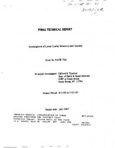
Figure 1. Transects (green lines) surveyed for cetaceans in the California Current Ecosystem by the SWFSC, 19912005.
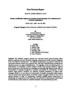
Figure 2. Transects (green lines) surveyed for cetaceans in the ETP by the SWFSC, 19862006.
6
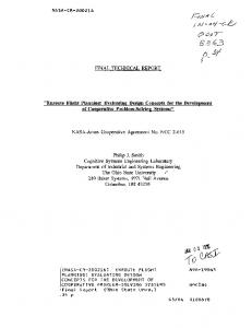
Figure 3. Completed transects for the winter/spring aerial line-transect surveys conducted off California in March-April 1991 and February-April 1992. The light gray line west and offshore of the aerial survey study area marks the boundary of the shipboard survey area within California.
The survey team consisted of four researchers: two “primary” observers who searched through the left and right bubble windows, a “secondary” observer who used the belly window to search the transect line and report sightings missed by the primary team, and a data recorder who entered sighting information and updated environmental conditions throughout the survey using a laptop computer connected to the aircraft’s LORAN or GPS navigation system. Following line-transect methods, perpendicular distances were calculated based on the declination angle to each sighting and the aircraft’s altitude. Surveys were flown at approximately 185 km/hr (100 knots) airspeed and 700 ft ASL altitude. When cetaceans were sighted, the aircraft circled over the animals to identify species and make group size estimates; any time the aircraft diverted from the transect was considered “off effort” and additional cetacean sightings made during this time were not included in the abundance estimates. These surveys were designed to estimate the abundance of cetaceans off California during the winter/spring period (Forney et al. 1995, Forney and Barlow 1998). Although there were insufficient sightings to develop cetacean-habitat models, these aerial survey data were 7
used to evaluate the ability of summer/fall models to predict winter/spring cetacean density patterns (Section 3.8). 3.1.2 In situ Oceanographic Measurements Oceanographic variables were measured on NMFS cetacean and ecosystem assessment surveys in the ETP during 1986-2006 and in the CCE during 1991-2005. Sea surface temperature (SST) and salinity (SSS) from a thermosalinograph were recorded continuously at 0.5 to 2 minute intervals and averaged over 5-10 km intervals to reduce both the number of observations and the discrepancy in sample spacing along and between transects. Thermocline depth (TD, depth of maximum temperature gradient in a 10 m interval), thermocline strength (TS, ºC m-1), and mixed layer depth (MLD, the depth at which temperature is 0.5ºC less than surface temperature) were estimated from expendable bathythermograph (XBT) and conductivitytemperature-depth (CTD) casts collected three to five times per day. Surface chlorophyll (CHL, mg m-3) was estimated at the same stations from the surface bottle on the CTD or from bucket samples analyzed by standard techniques (Holm-Hansen et al. 1965). CHL was log-transformed (using natural logarithms) to normalize the data for interpolation. Details of the field methods can be found in Philbrick et al. (2001, 2003). 3.1.3 Remotely Sensed Oceanographic Measurements Remotely sensed sea surface temperature (SST) data were considered for models within the California Current Ecosystem. Models included SST and measures of its variance as potential predictors. SST data (National Oceanic and Atmospheric Administration/National Environmental Satellite, Data, and Information Service/Pathfinder v5) were obtained via an OPeNDAP server using Matlab code that enabled remote, automated downloading of data for user-specified positions and resolutions. As part of this analysis (Becker 2007), we examined the predictive power of six different spatial resolutions of satellite SST data ranging from one pixel (approximately 31 km2) to 36 pixels (approximately 1,109 km2). Three temporal resolutions were also compared: 1) 1-day, 2) 8-day, and 3) 30-day composites. We used the coefficient of variation of SST, CV(SST), for resolutions greater than one pixel as a proxy for frontal regions in the California Current study area. Results are summarized below and details can be found in Becker (2007). Our SST temporal resolution analysis for the satellite-derived data indicated that, while 30-day SST composites had good within-dataset explanatory ability, predictive ability across datasets was poor at this coarser temporal resolution. A correlation analysis showed high correlation between the 1-day and 8-day SST values (R2 = 0.96), indicating that the 8-day composites provided adequate representation of average conditions on the day of the survey. Based on this evaluation and the greater availability of 8-day composite data compared to 1-day composites, we selected 8-day running average SST composites, centered on the date of each survey segment. 8
The SST spatial resolution comparison indicated that, for the majority of species, the greatest predictive ability was observed for the coarsest SST spatial resolution (Table 1). The predictive ability of different spatial resolutions of satellite-derived CV(SST) was more variable than that of SST. For many species, the best CV(SST) spatial resolution was among the finer resolutions considered in this study, perhaps reflecting the importance of localized upwelling events or small-scale frontal features. Table 1. Summary of satellite-derived sea surface temperature (SST) and CV(SST) spatial resolutions selected for ten California Current Ecosystem species. Numbers refer to the number of pixels included in the resolution. The spatial resolutions tested included 1, 4, 9, 16, 25, and 36 pixels, corresponding to 5.55-33.3 km boxes (i.e., 30.8 – 1,108.9 km2). Models are described in more detail in Section 3.3.
Past studies have shown relationships between cetacean sightings and other remotely sensed measures such as chlorophyll (Smith et al. 1986, Jaquet et al. 1996, Moore et al. 2002). However, satellite-derived measures of chlorophyll concentration were not available for 3 of the 4 survey years used to develop our CCE habitat models. The Coastal Zone Color Scanner (CZCS), one of the first satellite sensors to collect ocean color data, ceased operation in 1986 and the Sea Wide-Field-of-View Sensor (SeaWiFS) began operating shortly after our 1996 cetacean survey was over. Since chlorophyll data were not available for most of our time series, we did not include this variable as a potential predictor in our habitat models. 3.1.4 Water Depth and Bottom Slope Water depth was derived from the ETOPO2 2-minute global relief data (U.S. Department of Commerce 2006), re-gridded to match the pixel resolutions used for modeling. Slope was calculated as the magnitude of the bathymetry gradient using the gradient operator tool in Generic Mapping Tools (Wessel and Smith 1998). Depth and slope values for each geographic location were obtained using the “sample” tool in ArcGIS (version 9.2, ESRI, Inc.). 9
3.1.5 Mid-trophic Sampling with Net Tows and Acoustic Backscatter Most of the readily available measures of oceanic habitats are from physical oceanographic measurements (such as temperature and salinity) and from lower trophic levels (such as chlorophyll concentration and primary production). Cetacean distributions are likely to be determined more by the distribution of their prey, which are typically mid-trophic level species. To determine whether data about mid-trophic species distributions can improve cetacean-habitat models, we sorted and analyzed net-tow data and analyzed acoustic backscatter data that were collected on SWFSC cetacean and ecosystem assessment surveys. Manta net tows were conducted on 10 SWFSC surveys of the ETP since 1987, and bongo net tows were conducted on eight surveys of the ETP and CCE since 1998 (Fig. 4). Manta tows are conducted at the surface, and bongo tows are conducted between the surface and 200 m depth. Sorting samples collected with manta and bongo tows is labor-intensive and requires approximately one year of processing after each cruise. Both types of tows provide ichthyoplankton abundance and diversity data, but zooplankton volume and cephalopod abundance and diversity are recorded only from bongo tow samples.
Acoustic backscatter is a method of remotely measuring the biomass of fish and zooplankton in the water column using sonar. Acoustic backscatter data were collected on SWFSC surveys of the ETP in 1998, 1999, and 2000 using a Simrad EQ-50 scientific echosounder operating at a frequency of 38 kHz. The individual acoustic signals (i.e., pings) were averaged in horizontal bins during data collection on these cruises. This averaging was done before noise was removed from the data and the individual signals were not retained. Concern about the potential bias created by including noise in the acoustic backscatter variables led to a change in data collection protocols, which was implemented for the 2001 and all subsequent assessment surveys. This change in protocol invalidated comparison between data 10
collected before and after 2001. Consequently, only net-tow and acoustic backscatter data collected after 2001 were used to build cetacean-habitat models (see Section 3.7).
Figure 5. Mean volume backscattering strength, Svmean, in six hour segments along the a) 2003 and b) 2006 transects surveyed by the NOAA ship David Starr Jordan in the eastern tropical Pacific, and c) 2001 and d) 2005 transects surveyed by the NOAA ships David Starr Jordan and McArthur in the California Current ecosystem.
A more powerful Simrad EK-500 with three frequencies (38 kHz, 120 kHz, and 200 kHz) was used on SWFSC surveys of the CCE in 2001 and 2005 and the ETP in 2003 and 2006. We developed a new two-step noise removal method to process these data, which resulted in higher quality acoustic backscatter variables. The first step of the method identifies and eliminates high intensity irregular noise; the second step of the method targets low intensity “drop-outs” or returns within a ping that are significantly lower than expected. We evaluated the effect of the two-step noise removal method on the Svmean (dB) and nautical area scattering coefficient (NASC) (m2/nmi2) in 0-500 m, 0-100 m, 100-200 m, 200-300 m, 300-400 m, and 400-500 m depth bins. The Svmean is the average of the volume backscattering strength data logged by an echosounder; the NASC is a measure of area, rather than volume, scattering. Areas with higher intensity returns (i.e., areas with more scatterers) are indicated by larger S vmean and NASC values. The results indicate that the method is effective at removing both high-intensity irregular noise and low-intensity drop outs. Its efficacy is greatest when the entire water column is examined (e.g., our 0-500 m depth bin) and when the NASC is used as the summary output 11
variable. Interpolated maps of the Svmean, calculated from 0-500 m at a six hour resolution are shown for the ETP and CCE in Figure 5. 3.2 Oceanographic Data Interpolation
For cetacean-habitat modeling, and predictions based on such models, we examined the use of interpolated estimates of oceanographic parameters to predict cetacean densities at unsampled locations. The interpolated estimates are a matrix or grid calculated from sample values. Inevitably, there are errors due both to interpolation across the spatial gaps between sample points and to measurement inaccuracy and imprecision We investigated whether the interpolation method affects the interpolated values and, if so, identified the optimal method for interpolating observed oceanographic data for use in predictive models. The best estimate of an independent variable at an unsampled point in space (and time) is derived from an interpolation of sampled data that minimizes both the influence of measurement or sampling error in the observations and error introduced by the statistical technique, either between observations or at edges. Below we report on 1) a comparison of interpolation methods for oceanographic observations used in cetacean-habitat modeling and 2) the production of yearly interpolated fields of these variables. Five smoothing interpolation methods were compared to evaluate their relative performance. We did not consider exact interpolators because their emphasis on “honoring the data” does not work as well in cases with sampling error. The smoothing interpolators considered were (Golden Software, 2002): Inverse Distance Squared - data are weighted during interpolation such that the influence of an observation declines with the square of the distance from the grid point. Kriging (ordinary kriging) – a popular method that produces visually appealing maps from irregularly spaced data by incorporating anisotropy and underlying trends in the observations so that, for example, high points might be connected along a ridge rather than isolated by bull's eye type contours. Local Polynomial - assigns values to grid points by using a weighted least squares fit to data within the grid point’s search ellipse. Radial Basis Function - a multiquadric method, considered by many to be the best among this diverse group of methods, that uses basis kernel functions, analogous to variograms in kriging, to define the optimal set of weights to apply to the data when interpolating a grid point. 12
Minimum Curvature - the interpolated surface is analogous to a thin, linearly elastic plate passing through each of the data values with a minimum amount of bending, although it is not an exact interpolator. For the comparison of interpolation methods, Surfer scripts (Golden Software) were used for data manipulation and interpolation. Three variables (SST, TD, CHL) from one ETP survey (2006) and one CCE survey (2005) were investigated. For each dataset, subsets of observations were selected and removed from the dataset, the remaining observations were interpolated, and the residuals of the omitted observations were calculated, where the residual is the difference between an omitted data value and the interpolated value (i.e., the predicted value) at that point. Two jackknife procedures were used to calculate the mean and standard deviation of residuals at each data point: 1) single: omit each observation one at a time and 2) daily: omit each ship-day of observations (typically five observations) one ship-day at a time. In general, the only resultant difference between these two procedures was that daily jackknife residuals were slightly greater than single jackknife residuals. For each variable, a variogram analysis estimated length scale (i.e., how rapidly variance changes with increased distance between sampling points), error variance or the nugget effect (this source of error can be due to measurement error or small scale heterogeneity in the system), and anisotropy (Table 2). Then, jackknifing and interpolation were performed with similar search parameters for each of the five interpolation methods (search radii in Table 3). No additional smoothing was performed for methods that allowed this in Surfer (radial basis function, minimum curvature). Grid resolution was one degree of latitude and longitude. Yearly fields (interpolated surfaces) were created from data collected annually on NMFS cetacean and ecosystem assessment surveys in both the ETP and CCE study areas. These estimates were for the development of cetacean-habitat models and (potentially) the prediction of cetacean density in any user-selected polygon. Yearly fields were calculated for five CCE surveys (1991, 1993, 1996, 2001, and 2005) and for ten ETP surveys (1986, 1987, 1988, 1989, 1990, 1998, 1999, 2000, 2003, and 2006).
13
Table 2. Variogram model results. Anisotropy constrained as described in the text; for the CCE, the angle = 30º to account for the orientation of the California coast.
CCE
Model (r2)
Nugget
Scale
Length
SST
Spherical (0.43)
0.72
5.37
7.85
SSS
Gaussian (0.73)
0.05
0.74
8.03
MLD
Quadratic (0.59)
80.1
156.9
5.54
TS
R. quadratic (0.84)
0.0031
0.0025
1.94
CHL
Spherical (0.24)
0.026
0.042
5.69
ETP
Model (r2)
Nugget
Scale
Length
SST
R. quadratic (0.20)
3.27
7.46
27.4
SSS
Gaussian (0.64)
0.96
2.16
38.0
TD
R. quadratic (0.96)
494
2.15e6
1561
TS
R. quadratic (0.75)
0.0075
0.0125
25.1
CHL
Gaussian (0.43)
0.012
0.0057
13.6
14
Table 3. Range of annual sample sizes (N) and search parameters for kriging of grid points. Search radii are in degrees latitude/longitude; the two values are for the x and y directions, rotated 30º for the CCE. The two values differ due to anisotropy and thus define a search ellipse around each grid point. Anisotropy was constrained as described in the text. Nmax is the maximum number of samples allowed to interpolate a grid point value.
CCE
N within study area
Search radii
N within search ellipses
Nmax
SST
1681 - 3736
1.5, 2
282 - 492
200
SSS
1631 - 3718
1.5, 2
280 - 490
200
MLD
166 - 427
2, 2.67
40 - 81
40
TS
166 - 427
2, 2.67
28 - 60
40
CHL
390 - 695
2, 2.67
68 - 146
40
ETP
N within study area
Search radii
N within search ellipses
Nmax
SST
1686 - 7551
15, 10
638 - 2417
400
SSS
1681 - 7551
15, 10
638 - 2417
400
TD
719 - 1368
15, 10.7
218 - 375
80
TS
719 - 1368
15, 7.5
179 - 310
80
CHL
489 - 1676
15, 7.5
117 - 442
80
3.3 Modeling Framework 3.3.1 GLM and GAM Models Cetacean population density predictions were derived from encounter rate and group size models developed within a generalized additive modeling framework developed by Hedley et al. (1999) and Ferguson et al. (2006a and b). We also examined alternative methods of computing density, including: 1) predicting density directly by creating a single cetacean-habitat model with 15
“number of individuals” as the response variable and 2) deriving density from a two-step process in which the probability of a species being present in a given habitat is multiplied by the expected number of individuals given favorable habitat. The primary reason we decided to use separate models to predict encounter rate and group size is that this approach breaks the process down into ecologically meaningful quanta: differences in distribution may arise from variability in group size or number of groups in a given region, with potentially different environmental factors affecting the variability in each model. The two-step process of computing the probability of presence and then multiplying by the expected number of individuals does not have this flexibility because environmental effects on encounter rate and group size are confounded in a single model. GAMs are commonly used to relate characteristics of a species, such as distribution or abundance, to environmental characteristics. A GAM may be represented as
(Hastie and Tibshirani 1990). The function g(μ) is known as the link function, and it relates the mean of the response variable given the predictor variables =E(Y|X1,…,Xp) to the additive predictor jfj(Xj). GAMs are nonparametric extensions of generalized linear models (GLMs). The components fj(Xj) in the additive predictor of a GAM may include nonparametric smooth functions of the predictor variables, whereas a GLM is composed of a linear predictor, jjXj, in which the terms j are constants. This difference between the additive and linear predictor allows GAMs to be more flexible than GLMs. Model Comparison Analysis When working with ecological data, it is often difficult to distinguish meaningful signals from noise arising from the unexplainable variability and complex interactions inherent in ecological systems. Even in the absence of noise, relationships among ecological variables rarely can be explained by simple mathematical equations. Working within the framework of generalized additive models may be useful for analyzing ecological data because the nonparametric model structure of GAMs provides flexibility in model building and fitting, often allowing GAMs to exhibit more fidelity to the data than alternative model structures. Nevertheless, there are disadvantages to GAMs. For example, if appropriate model building and selection methods are not used, the resulting GAM may overfit the data, reliably reproducing the data upon which the model was built at the cost of sacrificing accuracy when predicting on novel data. In addition, GAMs may be difficult to interpret because they cannot always be defined by a simple formula comprised of a constant coefficient tied to each explanatory variable that indicates the strength, magnitude, and direction of the covariate’s effect on the response variable. 16
Finally, because the smoothing splines in the additive predictor are functions of the data used to build the model, predicting on novel data is not straightforward. We tested three different algorithms for constructing GAMs using a common set of environmental and cetacean linetransect survey data to evaluate how each approach addressed these problems. We also compared output from the GAMs to that produced by comparable GLMs to address whether the additional complexity of GAMs is warranted. In the model comparison analysis, three GAM algorithms and one GLM algorithm were tested: 1. S-PLUS gam (version 6 for Windows) with cubic smoothing splines of up to three degrees of freedom. Variable selection was implemented by step.gam using forward/backward stepwise selection with AIC. 2. R (version 2.6.2) gam from package gam with cubic smoothing splines of up to three degrees of freedom. Variables were selected by step.gam from package gam using forward/backward stepwise selection with AIC. 3. R (version 2.6.2) gam from package mgcv (version 1.3-29) using cubic regression splines (specified as bs = “cs”) and thin plate regression splines (bs = “ts”) with shrinkage. Variable selection in mgcv does not take a stepwise approach; rather, a smoothing parameter, which determines the effective degrees of freedom, is estimated for each predictor variable by minimizing the Generalized Cross Validation (GCV) score (Wood 2006). The gam.method argument to mgcv’s gam function specifies which numerical method is used to optimize the smoothing parameters. We tested six different gam.method options, namely outer, perf.outer, perf.magic, and perf.mgcv to construct the encounter rate models, and magic and mgcv to construct the group size models. Because GCV is known to select models that are overfit on occasion (Kim and Gu 2004), we tested two values of the parameter gamma that mgcv uses to compute GCV. Larger values for gamma penalize model complexity more than smaller values, so we tested the default, gamma = 1.0, and an alternative, gamma = 1.4. 4. R (version 2.6.2) glm from package stats with polynomial terms of up to three degrees of freedom. Variable selection was implemented by a forward/backward stepwise selection algorithm with AIC using the step.gam function from package gam. The use of polynomials allowed a degree of non-linearity between predictor and response variables in these linear models.
17
Encounter Rate and Group Size Models For each species or species group, we built separate models of cetacean encounter rate (number of sightings per unit of effort on the transect) and group size (number of individuals per sighting). In preparation for building the models, the cetacean sighting data and environmental data were summarized into segments of on-effort transect. Encounter rate models were built using all transect segments, regardless of whether they contained sightings. Group size models were built on only the subset of segments that contained sightings. Cetacean sighting data are essentially count data with relatively more zeroes than expected from a standard Poisson distribution. Therefore, we modeled encounter rate as a quasipoisson distribution with variance proportional to the mean and a logarithmic link function. The natural logarithm of segment length was included as an offset term to standardize each sample for effort. Cetacean group sizes can be highly variable, spanning up to three orders of magnitude. Estimating the mean group size associated with each line segment involved three steps. First, we computed an estimate of group size for each observer for each sighting based on the observer’s best, high, and low estimates of group size. Second, we computed the arithmetic mean of all observer’s group size estimates for each sighting. Finally, we computed the arithmetic mean group size of all sightings in each line segment. This three-step process resulted in non-integer group size estimates. Given the wide range of cetacean group sizes and the fact that the group size estimates are continuous data, we constructed lognormal GAMs for group size, using the natural logarithm of group size as the response variable and an identity link function. It was necessary to apply a bias-correction factor to the group size predictions from the GAMs because the models were built in log space and then the results were transformed back to arithmetic space, converting the group size estimate to a geometric mean in the process (Finney 1941, Smith 1993). The ratio estimator was used to correct for this back-transformation bias (Smith 1993). Density Computations To estimate cetacean density, the encounter rate and group size model results were incorporated into the standard line-transect equation:
where, n/L = encounter rate (number of sightings per unit length of transect), S= expected (or mean) group size, 18
ESW = effective strip width (one-sided), or 1/f(0), where f(0) is the sighting probability density at zero perpendicular distance g(0) = probability of detecting an animal on the transect line. Estimates of f(0) and g(0) were derived from previously published studies, as described in Section 3.5.
3.3.2 CART Tree-based Models We also applied Classification and Regression Trees (the CART algorithm in S-PLUS) to build a regression tree using the encounter rate data, but we found that the method was not appropriate for two reasons. First, it was not able to handle the zero-rich dataset. Second, the predictions were categorical not continuous, constrained to fall into one of the categories of observed encounter rate. Other methods of machine learning may perform better or provide additional insights for cetacean-habitat modeling, and further investigation is warranted.
3.4 Model Scale: Resolution and Extent
The results of spatial modeling often depend on the scale used. A pattern or relationship seen at one scale may be entirely different if viewed at a different scale (Wiens 1989). The choice of scales within a model must be appropriate to the questions being asked and the variation of the object being modeled. One aspect of scale is spatial resolution, which refers to the physical dimension of the smallest unit being studied. In the case of cetacean line-transect surveys, resolution refers to the length of the transect segments for which densities are estimated. The number of sightings of a species or the group size within each segment is the response variable (or dependent variable) which is predicted by the model. The predictor variables (or independent variables) used in the model to predict cetacean density would ideally be measured on the same scale, but may be measured on a smaller scale (in which case values can be averaged) or on a larger scale (in which case values can be interpolated). We examined the effect of resolution on models of cetacean encounter rates and group sizes by building models using a range of segment sizes. Specifically, we examined spatial resolutions from 2 to 120 km in both the ETP and the CCE. Habitat is expected to be more spatially heterogeneous in the CCE. A detailed description of the modeling technique used in both ecosystems can be found in Redfern et al. (2008). Another aspect of scale is extent, which refers to the maximum area being studied. Our study areas encompass what are considered to be two distinct ecosystems: the eastern tropical Pacific and the California Current. We explored the effect of extent by comparing models that 19
were built separately for each of these ecosystems with a model that was built using pooled data from both ecosystems. Modeling methodology followed Redfern et al. (2008), but only the 60km resolution was used.
3.5 Model Selection
Model validation using an independent data set is an integral part of building robust cetacean-habitat models (Forney 1997 and 2000, Becker 2007). In this analysis, final models for the CCE and the ETP were selected using a two-part process in which models were initially built using stepwise variable selection based on the available SWFSC survey data through 2003. Candidate models were then evaluated in terms of their predictive capabilities when applied to data from the novel 2005 (CCE) and 2006 (ETP) SWFSC cetacean surveys (see 3.1.1 Marine Mammal Surveys). Predictions and overall model performance were compared to identify the best models. A collection of quantitative and qualitative methods were used to compare models. Average squared prediction error (ASPE) was used to assess each model’s prediction accuracy across all segments (n) within the entire study area, where
Prediction accuracy was addressed in a spatial context using ratios of observed to predicted number of sightings (for the encounter rate models) or group size within each geographic stratum. These geographic strata were defined to be large enough to encompass a sufficient number of observations for a meaningful comparison of model predictions, yet environmentally distinct in terms of the biological and physical processes that determine habitat. In addition to examining the observed-to-predicted ratios themselves, we computed the sum of absolute deviations of the observed-to-predicted ratios, defined as
observed
1 predicted , where the sum is taken over all geographic strata used in model evaluation. For both the ASPE and observed-to-predicted ratio computations, the Beaufort sea state variable was set to the observed value to generate encounter rate and group size predictions. Explained deviance, the likelihood analogue of explained variance, was used to assess each model’s fit to the assumed distribution for the data. Model complexity was evaluated by examining the number of predictor variables selected and their associated degrees of freedom, in conjunction with visual inspection 20
of the smooth functions relating the effects of each predictor variable to the response variable. Finally, density predictions derived from the encounter rate and group size models were plotted on a map of the study area and the spatial distribution was evaluated by eye. Following model selection and validation, the best models were then re-fit to the additional year of data to parameterize the final predictive models. Details on the methods used to select and validate our final models within each geographic region are provided below. 3.5.1 California Current Ecosystem Models In preparation for model selection and validation using the 2005 west coast survey data, in situ models built at scales of 2 and 10 km for the scale analyses (see Section 3.4 Model Scale: Resolution and Extent) were compared to 5 km models built with remotely sensed data (Becker 2007). For each species, we compared key predictor variables and associated functional shapes, study area density ratios (density calculated using standard line-transect methods divided by density predicted by the habitat model), standard errors (SE) of density ratios, and average squared prediction errors (ASPE). We found that the models built with remotely sensed data performed as well or better than the models built with in situ data. However, for some species the in situ oceanographic variables had a large effect on one or both response variables (encounter rate and group size) relative to the other predictors. Based on these analyses, we developed two sets of CCE models at the 5 km scale: 1) a set that included only remotely sensed habitat variables, and 2) a set that included a combination of in situ and remotely sensed predictor variables. These two types of models were subsequently compared to develop and finalize models on a species-specific basis. Initial Model Selection and Evaluation Process Initial models for both the in situ and remotely sensed data sets were selected using a “pseudo-jackknife” cross-validation approach (Becker 2007). Specifically, three data sets were constructed by excluding one of the four survey years available for model building (1991, 1993, 1996, and 2001). [Note: Data collected during 1993 were included in all model combinations because 1993 was the year with the warmest mean sea surface temperatures and was considered essential to capture the observed inter-annual variability in oceanographic conditions.] Each model was then used to predict the excluded year, and ASPE was calculated. This process of cross validation on all model combinations produced four ASPE values for each of the six initial models (three encounter rate models and three group size models). The paired models with the lowest sum of ASPE values (i.e. with lowest prediction errors across all survey years) were selected as the best overall models. Group size and encounter rate models were constrained to be paired because preliminary analyses indicated that variable selection was not independent; an increase in animal densities (e.g., with higher sea surface temperature) could be reflected in either a higher encounter rate or larger groups, and this effect varied among years. If models were built from different yearly subsets, this could result in the loss or overrepresentation of one or more variables, causing bias. 21
Expanding models to the entire U.S. West Coast All of our initial west coast analyses (e.g., scale evaluation, seasonal predictions, etc.) were based on models developed using survey data collected only in California waters in 1991, 1993, 1996, and 2001, because Oregon and Washington waters were not surveyed in 1991 and 1993 and it was important to capture the greatest degree of inter-annual variability possible. Using four years of California-only data provided the most robust data set for construction of models, model validation, and other associated analyses. However, the inclusion of waters off Oregon and Washington in the final West Coast Spatial Decision Support System (SDSS) required a new approach to model selection, because the pseudo-jackknife cannot be used when regional coverage is unequal, and the varying survey extent could result in biased models. Therefore, we explored alternate 'best model' selection criteria for models encompassing the entire West Coast study area. First, we compared key predictor variables and associated functional shapes of independent models built with California only vs. Oregon and Washington data. Based on the similarities of the variables and their functional forms, we concluded that we could combine the datasets for model building without introducing bias. This approach has the advantage of maximizing sample sizes and building models based on a broader range of environmental conditions. We then selected the five models that minimized AIC, and chose the best model based on non-AIC criteria applied to each individual survey year and the collective data set. These criteria included density ratios (line-transect derived density divided by predicted density) and a visual evaluation of spatial patterns in the model compared to the sighting data. For evaluation purposes, we built nested models for six species using only the California survey data. The species selected represented a broad range of habitat preferences: short-beaked common dolphin (Delphinus delphis), Risso’s dolphin (Grampus griseus), northern right whale dolphin (Lissodelphis borealis), Dall’s porpoise (Phocoenoides dalli), fin whale (Balaenoptera physalus), and humpback whale (Megaptera novaeangliae). Models constructed for California waters using these methods were similar or identical to those selected using the pseudo-jackknife procedure; therefore, this alternate selection process was used for the final West Coast model development. Two candidate 'pre-final' models were developed for each species: one built only with remotely sensed habitat variables and another built with a combined set of in situ and remotely sensed predictor variables (“combined” models). Habitat predictor variables Predictor variables for the remotely-sensed models included sea surface temperature (SST), the coefficient of variation (CV) of SST within a 6x6 pixel (1,109 km2) box (to serve as a proxy for frontal regions; Becker 2007), water depth, bathymetric slope, distance to the 2,000 m 22
isobath, and Beaufort sea state. Distance to the 2,000 m isobath was added to the list of predictors because sighting plots suggested that this variable could potentially improve model performance for some species (e.g., sperm whale, Physeter macrocephalus, and Baird’s beaked whale, Berardius bairdii) that are generally found only in slope or deep waters. This variable was coded to indicate whether the location was deeper (-) or shallower (+) than the 2,000 m isobath. Beaufort sea state affects the probability of detecting animals (Barlow et al. 2001), and the average observed sea state value on each segment was included as a continuous predictor variable in our models in order to account for sighting conditions. In addition to the variables used for the remotely-sensed models, the combined models included three potential predictors derived from data collected in situ: sea surface salinity, the natural logarithm of surface chlorophyll concentration, and mixed layer depth, measured as the depth at which the water temperature was 0.5C less than at the surface. Remotely sensed measures of SST and CV(SST) were used in the combined models because the remotely-sensed CV(SST) was found to be more effective at characterizing frontal regions than our in situ CV(SST) measures (Becker 2007), and SST measures performed similarly. The in situ data were derived in one of two ways. Salinity was sampled continuously along the transect and segmentspecific estimates were obtained by averaging values within 5 km of the mid-point of each transect segment included in the analysis. Chlorophyll and mixed layer depth were measured much less frequently, and a linear interpolation between nearby stations did not accurately capture values at the edges of the study area or when samples were sparse, causing 'bull’s eye' effects in estimated cetacean density. Therefore, the data were first contoured (see Section 3.2) to provide a 2-D surface of estimated chlorophyll and mixed-layer depth values, and segment mid-point values were extracted from the contour grid using the Surfer 8.0 (Golden Software, Inc) Residuals feature. Density Estimation Segment-specific density estimates were derived by incorporating the predicted values for encounter rate and group size into the standard line-transect equation (Buckland et al. 2001) as described by Becker (2007) and in Section 3.3.1. We relied on published values of detection probability (f(0) and g(0)) for each species as estimated from the same survey data used for model development (Barlow 2003). Published values for many species were stratified by group size and, for purposes of estimating densities, we incorporated weighted f(0) and g(0) values based on the number of small and large groups observed during the surveys (Becker 2007, Table 4). All final model predictions were made using the average observed Beaufort sea state for conditions 0-5 during the SWFSC cruises. This is appropriate because it corresponds to the conditions for which the line-transect parameters f(0) and g(0) were estimated (Barlow 2003). For Dall’s porpoise and small beaked whales, published f(0) and g(0) values were available only for Beaufort conditions of 0-2. Model predictions for this species and guild were made using the average observed Beaufort sea state for conditions 0-2. 23
Table 4. Summary of the weighted effective strip width (ESW = 1/ f(0)) and g(0) estimates used to calculate predicted densities for the CCE. The original values are those estimated from the 1991-2001 survey data (Barlow 2003), which included both perception and availability bias to the extent possible. These values are weighted by the number of small and large groups observed during the 1991, 1993, 1996, 2001, and 2005 surveys. ESW g(0) Group size original weighted original weighted Striped dolphin 1-20 0.50 0.77 0.97 0.89 21-100 1.24 1.00 100+ 1.88 1.00 Short-beaked common dolphin 1-20 0.50 0.77 21-100 1.24 1.32 1.00 0.95 100+ 1.88 1.00 Risso’s dolphin 1-20 1.37 0.74 20+ 2.18 1.63 1.00 0.82 Pacific white-sided dolphin 1-20 0.50 0.77 21-100 1.24 0.92 1.00 0.86 100+ 1.88 1.00 Northern right whale dolphin 1-20 0.50 0.77 21-100 1.24 0.78 1.00 0.84 100+ 1.88 1.00 Dall’s porpoise all 0.82 0.82 0.79 0.79 Sperm whale all 4.61 4.61 0.87 0.87 Fin whale all 1.72 1.72 0.90 0.90 Blue whale all 1.72 1.72 0.90 0.90 Humpback whale all 2.89 2.89 0.90 0.90 Baird’s beaked whale all 2.83 2.83 0.96 0.96 Small beaked whales all 1.76 1.76 0.34* 0.34 * Based on average g(0) for Mesoplodon (Mesoplodon spp.) and Cuvier’s beaked whales (Ziphius cavirostris). Species
Final CCE Model Selection As described above, we developed two candidate “pre-final” CCE models for each species: one built with remotely sensed habitat variables, and one 'combined' model built with both remotely sensed data and interpolated in situ data (see Section 4.1). Initially, models were built for the ten species with the greatest number of sightings in order to provide the most robust environmental models: striped dolphin (Stenella coeruleoalba), short-beaked common dolphin, Risso’s dolphin, Pacific white-sided dolphin (Lagenorhynchus obliquidens), northern right whale dolphin, Dall’s porpoise, sperm whale, fin whale, blue whale (Balaenoptera musculus), and humpback whale. As part of the final model selection process, we convened an expert workshop to solicit feedback on the pre-final spatial models for both the CCE and ETP study areas. The scientists who participated in the workshop all have significant field and research experience within these oceanic regions and are recognized for their extensive knowledge of cetacean distributions in the study areas. The experts were shown maps with smoothed density predictions for 10 species in 24
the CCE and 15 species in the ETP. At least two maps were presented for each species; competing maps varied either by the predictor variables included in the models (CCE) or by the analytical methods used to develop the models (ETP). The experts provided comments and participated in open discussions regarding the ability of the models to capture known distributions for each species. For those cases where the maps failed to capture overall distribution patterns, the experts provided input on predictor variables that might be included in future models to increase their predictive ability. For species like Risso's dolphins whose modeled density plots did not appear to capture major distribution patterns, the experts suggested that it would be worth investigating the performance of a model that included one or two static variables, such as categorical stratum variables. Based on workshop discussions, we built CCE habitat models for two additional species/guilds: Baird's beaked whale, and small beaked whales (Ziphius and Mesoplodon).
Figure 6. Geographic strata used for the CCE spatial predictions. The eight strata include waters inshore and offshore of the 2000 m isobath in Oregon/Washington, Northern California, Central California, and Southern California.
In addition to input received at the expert workshop, final model selection was based on a comparison of the models’ ability to predict on a novel dataset. We compared total study area density ratios and standard errors (SEs) of density ratios for the competing models’ 2005 predictions. In addition, these measures were compared to those of predictions made on the individual years that went into the model building. We also included a spatial measure of model performance in our evaluation by looking at the density ratios on a geographically stratified basis. To facilitate the spatial analysis, we stratified the study area into eight regions (Fig. 6). 25
Consistent with Barlow and Forney (2007), we created four northern/southern strata: waters off Oregon and Washington (north of 42°N), northern California (south of 42°N and north of Point Reyes at 38°N), central California (south of Point Reyes and north of Point Conception at 34.5°N), and southern California (south of Point Conception). These regions were further stratified into western and eastern regions at the 2,000 m isobath. Therefore, we were able to evaluate spatial predictions on a yearly basis as well as for all years combined. In addition, inspection of predicted species density maps overlaid with survey sighting locations provided a means for qualitatively comparing the models’ predictions. Density Interpolation The segment-specific predictions from the model were interpolated to the entire study area using Surfer 8.0 (Golden Software, Inc). For the California Current models, interpolation grids were created at a resolution of 25 km, using inverse distance weighting to the power of 2. This weighting method gives points closer to each grid node greater influence than those farther away. All data within a search radius of 2 degrees latitude (222 km) were used for interpolation, because transect spacing ranged from 150 to 230 km during the five different survey years, and contouring results were more robust when data from more than one transect line were included. Grids were created for each of the individual survey years (1991, 1993, 1996, 2001, and 2005) for the California Current Ecosystem. Subsequently, the individual grid cells were averaged across all years to calculate mean species density and its variance. To eliminate occasional over-specification ('bull’s eye' effects) in the final average prediction grid, a 5x5 pixel moving average filter with equal weights was applied to the entire grid. The complete gridding process provided smoothed multi-year average cetacean densities, taking into account both the varying oceanographic conditions and different levels of sampling coverage achieved during the SWFSC cetacean surveys. Standard errors and upper and lower lognormal 90% confidence limits were calculated from the grid cell averages and variances using standard formulae. Following selection of the final models, we performed an abundance cross-check to further validate model predictions. We compared the final model overall study area density predictions to the Barlow (2003) estimates derived using line-transect analyses to examine potential bias. Although the estimates provided by Barlow (2003) also have uncertainty associated with them, they provide a benchmark against which our model predictions can be evaluated. If the model-based estimate was substantially different from the line-transect estimate, we re-examined the model and performed additional analyses as necessary. In sum, evaluation factors used to select and validate our final models included expert opinion, temporal and spatial density ratios (including novel dataset predictions), density plots reflecting both yearly and averaged predictions, and abundance cross checks.
26
3.5.2 Eastern Tropical Pacific Models Data Extraction Data used for constructing and validating ETP cetacean-habitat models were collected during SWFSC cruises to the eastern tropical Pacific between 1986 and 2006. Sufficient sample sizes were available to build GAMs for 15 species or guilds: offshore spotted dolphin (Stenella attenuata), eastern spinner dolphin (Stenella longirostris orientalis), whitebelly spinner dolphin (Stenella longirostris longirostris), striped dolphin, rough-toothed dolphin (Steno bredanensis), short-beaked common dolphin, bottlenose dolphin (Tursiops truncatus), Risso’s dolphin, Cuvier’s beaked whale, blue whale, Bryde’s whale (Balaenoptera edeni), short-finned pilot whale (Globicephala macrorhynchus), dwarf sperm whale (Kogia sima), Mesoplodon beaked whales (including Mesoplodon spp., Mesoplodon densirostris, and Mesoplodon peruvianus), and small beaked whales (Mesoplodon beaked whales plus “unidentified beaked whale”). Only data from surveys conducted after 1990 were used to construct the offshore spotted dolphin models because Stenella attenuata was not distinguished from the coastal spotted dolphin, Stenella attenuata graffmani, in the earlier survey years. Table 5 lists summary statistics for each species. To build the ETP encounter rate and group size GAMs, line-transect survey data were divided into segments of approximately 10 km of on-effort transect. The potential predictor variables included closest distance to shore (continents or islands), depth, and in situ oceanographic data collected during the line-transect surveys, specifically, sea surface temperature (SST), sea surface salinity (SAL), mixed layer depth (MLD), and the natural logarithm of the surface chlorophyll concentration (CHL). In addition, the average Beaufort sea state on each segment was considered as a potential predictor variable in all models to account for potential biases due to visibility. Although it is possible to account for the sea state visibility bias elsewhere in the density analysis, including Beaufort as a predictor variable in the generalized additive model automatically accounts for correlations among other predictor variables. Furthermore, the Beaufort covariate in the encounter rate models provides information about the segments in which zero sightings were made that can be used to distinguish poor habitat from data collected during poor visibility conditions. Only survey effort conducted in Beaufort sea state condition of 5 or less was used to build the models. Latitude and longitude were initially omitted from all models because they are static predictors that do not reflect the dynamic environment in which these cetaceans live, bringing into question the ability of these covariates to accurately predict densities from novel data. The only species for which latitude and longitude were included in the final model was the eastern spinner dolphin because its distribution is contiguous with the whitebelly subspecies of spinner dolphin. The habitat occupied by the eastern spinner dolphin might be affected by the distribution of whitebelly spinners in addition to other physical and biological characteristics of the environment; 27
incorporation of geographic coordinates into the model is a simple way to account for this relationship.
Table 5. Total number of sightings used to build, validate, and parameterize the final models for the ETP. The sightings used to build the initial models are from the SWFSC’s 1986, 1987, 1988, 1989, 1990, 1998, 1999, 2000, and 2003 surveys of the ETP. Sightings from the SWFSC survey in 2006 were used to validate the best models. The best models were re-fit to the additional year of data to parameterize the final predictive models. Numbers reflect sightings made in Beaufort sea states of 0-5 and for which in situ data were available.
Guild Offshore spotted dolphin Eastern spinner dolphin Whitebelly spinner dolphin Striped dolphin Rough-toothed dolphin Short-beaked common dolphin Bottlenose dolphin Risso's dolphin Cuvier's beaked whale Blue whale Bryde's whale Short-finned pilot whale Dwarf sperm whale Mesoplodon spp. Small beaked whales
Total number of sightings build validate re-fit 886 116 1002 395 62 457 168 16 184 1081 124 1205 212 34 246 423 66 489 626 87 713 250 25 275 116 9 125 74 35 109 267 29 296 296 58 354 99 13 112 116 14 130 257 26 283
Oceanography values for each segment were calculated as weighted averages of the oceanography data collected on the same day as, and within a radius of 50 km of, each segment midpoint. Inverse distance weighting (distance -1) was used in the weighted average computations. GAM Model Construction Encounter rate and group size models for the ETP were constructed using survey data from 1986, 1987, 1988, 1989, 1990, 1998, 1999, 2000, and 2003. All models were created using the R (version 2.6.2) mgcv package (version 1.3-29), as described under Model Comparison Analysis in Section 3.3. Models containing univariate smooths were constructed first. Interactions were introduced on a case-by-case basis to improve model fit and predictive ability.
28
The eastern spinner dolphin was the only species for which interactions were included in the GAMs. Model Evaluation For each guild and response variable, a “simple” and a “complex” model were compared using ASPE and ratio criteria for the geographic strata shown in shown in Figure 7. The “simple models” had relatively few effective degrees of freedom and the smallest sum of absolute deviations of the observed-to-predicted ratios. Similarly, the “complex models” represented those having a relatively large number of effective degrees of freedom in addition to good agreement between observed and predicted values of the response variable. For cases in which a single model clearly outperformed all of the others, only one model was selected.
Figure 7. Geographic strata used for ETP model selection and validation. WBP: West Baja Peninsula. GOC: Gulf of California. NEC: North Equatorial Current. NECC: North Equatorial Countercurrent. EWP: Equatorial Warm Pool. CRD: Costa Rica Dome. ECT: Equatorial Cold Tongue. Coast: Coastal stratum (separated from other geographic strata only for the offshore spotted dolphin analysis).
As discussed above under Final CCE Model Selection for the California Current ecosystem, we convened a workshop for cetacean experts to solicit feedback on preliminary model results. We incorporated all of the experts’ comments into the final models, as summarized below:
Build a model for “small beaked whales” that includes all sightings for the genus Mesoplodon, in addition to “unidentified small beaked whale” sightings.
Include sightings of “Bryde’s or sei (Balaenoptera borealis) whales” in the Bryde’s whale model. Bryde’s and sei whales can be difficult to distinguish from a distance, but the 29
overwhelming majority of “Bryde’s or sei whale” sightings in the ETP region are Bryde’s whales.
Include sightings of “Kogia spp.” in the Kogia sima model because the majority of Kogia sightings unidentified to species in the ETP are believed to be K. sima.
Do not include Beaufort sea state as a predictor variable in the spotted dolphin models because the primary visual cue for Stenella attenuata sightings is flocks of birds flying overhead.
Incorporate latitude and longitude, or a latitude/longitude/SST interaction term in the eastern spinner model to differentiate eastern spinner from whitebelly spinner habitat.
Include islands in the distance-to-shore computation to improve the prediction accuracy of the bottlenose dolphin encounter rate models in particular.
Select simple models for the final models, unless strong support exists for the alternative complex model.
Use geographically stratified estimates of density rather than predictions derived from cetacean-habitat models for sperm whales, killer whales (Orcinus orca), and coastal spotted dolphins.
Image Quality Analysis (IQA; Wang et al. 2004), a quantitative, spatially-explicit method for comparing two images, was implemented as an additional model evaluation technique, but it was not used in final model selection because we found that people had difficulty interpreting the resulting statistics. Nevertheless, the IQA approach seems promising and future work into making the results accessible to a non-expert audience would be valuable. Density Estimation The values for the line-transect sighting parameters f(0) and g(0) used to compute population density in the ETP analysis came from published reports, as summarized by Ferguson and Barlow (2001). For species in which the f(0) values were stratified by group size, selection of the appropriate group size stratum for determining which value of f(0) to use was determined by the group size predictions from the preferred group size model for the species. Similar to the California Current analysis, the value of Beaufort sea state used to compute the final encounter rate and group size predictions for the SDSS was set to the average Beaufort, weighted by survey effort, of all segments used to build the models. The f(0) values for all beaked whales and Kogia were computed from data collected during Beaufort sea states from 0 to 2. Therefore, computation of weighted average Beaufort for beaked whales and Kogia predictions included only segments with average Beaufort conditions of 2 or less. 30
Encounter rate and group size were predicted to segment midpoints located directly on the survey transects, and the resulting densities were interpolated (as described under Density Interpolation in the California Current section above) to provide gridded density predictions throughout the study area. Grids were created for each of the individual survey years (19861990, 1998-2000, 2003, and 2006) and interpolated at a resolution of 100 km. All data within a search radius of 10 degrees latitude (1,111 km) were included in the inverse distance weighting calculations. Model Validation Data from the 2006 line-transect surveys in the ETP were used to validate the encounter rate and group size models constructed using data from 1986-2003. Data processing for this model validation task followed that described under Data Extraction for the ETP above. To assess the models’ fit to the validation data set and to examine the inter-annual variability in model predictions, density was predicted separately for each survey year from 1986 to 2006. Methods used to evaluate model fit included visual inspection of geographic contour plots of the annual density predictions and computation of geographically stratified ratios of observed to predicted density. 3.5.3 Line-transect densities for unmodeled species The predictive habitat models described above were developed for all ETP and CCE species with sufficient sightings and survey data during the summer/fall season. Several additional species were observed during the surveys, but too few observations were made to develop models. Similarly, a SWFSC survey of waters surrounding Hawaii yielded too few sightings for modeling of cetacean densities in that region. Therefore, constant densities were derived for these species and regions, based on published line-transect estimates applied to the most appropriate species-specific strata. Coefficients of variation and lognormal 90% confidence limits were estimated from the published CVs, or re-calculated for specific strata using the same methods as the original studies. Within the California Current Ecosystem, line-transect estimates derived from the 19912005 U.S. West Coast surveys (Barlow and Forney 2007; Table 6) were used for the following species during summer: long-beaked common dolphin (Delphinus capensis), short-finned pilot whale, bottlenose dolphin, killer whale, minke whale (Balaenoptera acutorostrata), Bryde's whale, sei whale, and a combined category for pygmy and dwarf sperm whales (Kogia spp.). Similarly, average winter densities estimated for cetaceans off California (Forney et al. 1995) based on aerial line-transect surveys were applied to appropriate geographic strata on a speciesspecific basis. These species included: common dolphins (Delphinus spp.), Pacific white-sided dolphin, northern right whale dolphin, Dall's porpoise, Risso's dolphin, bottlenose dolphin, killer whale, blue whale, fin whale, humpback whale, sperm whale, minke whale, North Pacific right whale (Eubalaena japonica) and a category of 'small beaked whales' which includes species of 31
the genera Ziphius and Mesoplodon. Constant line-transect densities for two additional coastal species that are present year-round were derived from published values: harbor porpoise (Phocoena phocoena; Carretta et al., in press), and coastal bottlenose dolphins (Dudzik et al. 2006, Carretta et al. 2007). Geographically stratified density estimates for the three unmodeled ETP cetacean species (killer whale, sperm whale, and coastal spotted dolphin) were taken from Ferguson and Barlow (2003) without further combining or splitting of strata (Fig. 8, Table 7).
Figure 8. Stratum numbers for ETP line-transect density estimates for coastal spotted dolphin, killer whale, and sperm whale (from Ferguson and Barlow 2003).
Estimates of abundance and density for Hawaiian cetaceans (Table 8) were largely derived from a 2002 shipboard line-transect survey (Barlow 2006). Although Barlow defined two geographic strata for the analysis (Main Hawaiian Islands and Outer EEZ), variance estimates were only provided for the combined Hawaiian EEZ area. For most species, density estimates were similar in the two geographic strata (with wide, overlapping confidence intervals), so a single EEZ-wide density and associated variance were considered appropriate. Three species, however, exhibited markedly higher densities within the Main Hawaiian Islands stratum. In these cases, stratum-specific density estimates were retained (to increase accuracy), and variance was approximated by assuming the coefficient of variation (CV) was equal to that estimated for the overall study area (likely underestimating the true variance). Lastly, Barlow and Rankin (2007) provided updated estimates of false killer whale abundance in Hawaiian waters, based on additional sighting data obtained during a 2005 Pacific Islands Survey.
32
Table 6. Geographically stratified estimates of abundance (N), density (D), coefficient of variation (CV), and lognormal 90% confidence intervals of density for unmodeled cetacean species in the California Current Ecosystem. CALIFORNIA CURRENT ECOSYSTEM Species Area N CV SUMMER ESTIMATES (Barlow and Forney 2007) Southern CA 17530 1.03 Long-beaked common dolphin Central CA 4375 1.03 Northern CA 0 Oregon and Washington 0 Southern CA 1831 0.47 Bottlenose dolphin Central CA 61 0.77 (offshore stock) Northern CA 133 0.68 Oregon and Washington 0 n/a Short-finned pilot whale California, Oregon, Washington 350 0.48 Killer whale California, Oregon, Washington 809 0.27 Minke whale California, Oregon, Washington 823 0.56 Bryde's whale California, Oregon, Washington 7 1.01 Sei whale California, Oregon, Washington 98 0.57 Pygmy/dwarf sperm whales California, Oregon, Washington 1237 0.45 WINTER ESTIMATES (Forney et al. 1995, variances re-calculated using same methods) Southern California Bight 272,101 0.373 Common dolphins Outer Southern CA waters 26,535 0.731 Central California 7,058 0.977 Northern California 0 Southern California Bight 2,654 0.659 Pacific white-sided dolphin Outer Southern CA waters 18,779 0.670 Central California 74,678 0.620 Northern California 25,583 0.956 Southern California Bight 6,381 0.369 Northern right whale dolphin Outer Southern CA waters 8,895 0.871 Central California 4,091 0.510 Northern California 1,966 0.893 Southern California Bight 1,582 0.393 Dall's porpoise Outer Southern CA waters 716 0.827 Central California 4,744 0.314 Northern California 1,418 0.427 Southern California Bight 9,396 0.405 Risso's dolphin Outer Southern California waters 636 0.990 Central California 22,343 0.637 Northern California 0 Southern California Bight (SCB) 3,165 0.501 Bottlenose dolphin California excluding SCB 95 1.032 (offshore stock) Killer whale California 65 0.689 Blue whale California 30 0.990 Fin whale California 49 1.012 Humpback whale California 319 0.407 Sperm whale California 892 0.990 Small beaked whales California 392 0.408 Minke whale California 73 0.616 North Pacific right whale California 16 1.110 YEAR-ROUND ESTIMATES (Carretta et al., in prep, Dudzik 2006, Carretta et al. 2007) Morro Bay Stock (inshore) 2066 0.4 Harbor porpoise Morro Bay Stock (offshore) 280 0.65 Monterey Bay Stock (inshore) 1354 0.4 Monterey Bay Stock (offshore) 324 0.8 SF/Russian River Stock (inshore) 8830 0.38 SF/Russian River Stock (offshore) 520 1.39 No. CA & So. OR Stock (inshore) 13291 0.44 No. CA & So. OR Stock (inshore) 837 0.69 Bottlenose dolphin (coastal stock) Within 1km of shore 358 0.13
33
D
L90%
U90%
0.05504 0.01800 0.00000 0.00000 0.00575 0.00025 0.00052 0.00000 0.00031 0.00071 0.00072 0.00001 0.00009 0.00108
0.01365 0.00446 0.00276 0.00008 0.00019 0.00015 0.00046 0.00031 0.00000 0.00004 0.00054
0.22200 0.07262 0.01196 0.00077 0.00142 0.00065 0.00109 0.00170 0.00002 0.00020 0.00219
5.87691 0.41609 0.05876 0.00000 0.05732 0.29447 0.62176 0.75045 0.13782 0.13948 0.03406 0.05767 0.03417 0.01123 0.03950 0.04160 0.20294 0.00997 0.18602 0.00000 0.06836 0.00062 0.00025 0.00011 0.00019 0.00121 0.00338 0.00148 0.00028 0.00006
3.25151 0.14229 0.01535 0.02141 0.10848 0.24401 0.20020 0.07671 0.04068 0.01548 0.01643 0.01835 0.00344 0.02389 0.02126 0.10710 0.00257 0.07143 0.03146 0.00015 0.00009 0.00003 0.00005 0.00064 0.00087 0.00078 0.00011 0.00001
10.62215 1.21678 0.22499 0.15348 0.79938 1.58427 2.81308 0.24762 0.47826 0.07494 0.20247 0.06361 0.03668 0.06531 0.08138 0.38454 0.03868 0.48443 0.14854 0.00249 0.00068 0.00044 0.00073 0.00229 0.01309 0.00282 0.00070 0.00026
0.9591 0.0617 0.9993 0.1504 1.8195 0.1033 3.6424 0.1146 0.3612
0.50991 0.02329 0.53123 0.04746 0.99626 0.01885 1.82707 0.04119 0.29209
1.80417 0.16324 1.87963 0.47671 3.32299 0.56587 7.26126 0.31892 0.44660
Table 7. Geographically stratified estimates of abundance (N), density (D), coefficient of variation (CV), and lognormal 90% confidence intervals of density for three ETP cetacean species. Stratum numbers are from Ferguson and Barlow (2003), shown in Figure 8. Coastal spotted dolphin Stratum N CV D L90% 85 11,327 0.64 0.0536 0.0205 103 394 1 0.0013 0.0003 118 11,297 0.55 0.0800 0.0344 119 239 1 0.0009 0.0002 137 10,148 0.48 0.0971 0.0460 138 771 0.71 0.0037 0.0013 158 4,473 0.71 0.0432 0.0152 179-181 3,070 0.58 0.0291 0.0120 Killer whale Stratum N CV D L90% 35-36 1,370 0.9 0.0030 0.0008 46 37 1 0.0003 0.0001 47-48 188 1 0.0004 0.0001 59 111 0.71 0.0004 0.0001 72 63 1 0.0002 0.0001 85 28 1 0.0001 0.0000 86 84 0.71 0.0003 0.0001 87 61 1 0.0002 0.0001 101-102 15 1 0.0001 0.0000 103 20 1 0.0001 0.0000 104 59 1 0.0002 0.0001 105 39 1 0.0001 0.0000 119 62 0.71 0.0002 0.0001 121 82 1 0.0003 0.0001 122 40 1 0.0001 0.0000 124 232 0.71 0.0008 0.0003 126 59 1 0.0002 0.0001 127 449 0.71 0.0015 0.0005 128-129 835 0.58 0.0014 0.0006 138 14 1 0.0001 0.0000 139 54 1 0.0002 0.0001 140 45 1 0.0001 0.0000 141 292 0.58 0.0010 0.0004 142 217 1 0.0007 0.0002 143 219 0.58 0.0007 0.0003 147 110 1 0.0004 0.0001 150-151 477 1 0.0008 0.0002 159 108 0.71 0.0004 0.0001 160 220 0.63 0.0007 0.0003 164 55 1 0.0002 0.0001 166 231 0.58 0.0007 0.0003 182 50 1 0.0018 0.0005 200 58 1 0.0002 0.0001 201 349 0.64 0.0011 0.0004 202 372 1 0.0012 0.0003 203 139 0.71 0.0004 0.0001 205 156 1 0.0005 0.0001 207 902 1 0.0029 0.0007 212 170 1 0.0006 0.0002 213 772 0.71 0.0025 0.0009 215-216 296 1 0.0005 0.0001 218-220 3,116 0.58 0.0040 0.0017
U90% 0.1401 0.0051 0.1859 0.0035 0.2049 0.0106 0.1232 0.0704 U90% 0.0106 0.0012 0.0016 0.0011 0.0008 0.0004 0.0009 0.0008 0.0004 0.0004 0.0008 0.0004 0.0006 0.0012 0.0004 0.0023 0.0008 0.0043 0.0034 0.0004 0.0008 0.0004 0.0024 0.0027 0.0017 0.0016 0.0031 0.0011 0.0018 0.0008 0.0017 0.0071 0.0008 0.0029 0.0047 0.0011 0.0020 0.0114 0.0024 0.0071 0.0020 0.0097
Stratum N 22-23 419 35-36 75 46 440 47-48 507 58 35 59 282 60 64 71 53 72 128 73 63 85 206 86 348 87 110 103 886 104 31 105 78 106 195 111-112 56 119 487 121 113 124 261 137 450 138 534 139 1,253 140 297 141 336 142 378 143 272 144 311 145 702 147 194 148 306 149 204 150-151 50 158 1,010 159 1,583 160 1,072 161 158 162 271 164 169 165 164 166 140 179-181 240 200 2,829 201 318 202 295 203 162 204 312 205 253 206 1,004 207 36 211 2,057 212 63 213 66 214 77 215-216 409 218-220 11,969
34
Sperm whale CV D 0.71 0.0017 0.71 0.0002 0.59 0.0035 0.47 0.0010 0.71 0.0003 0.42 0.0011 1 0.0002 0.71 0.0008 0.43 0.0005 1 0.0002 0.71 0.0010 0.53 0.0013 1 0.0004 0.72 0.0030 0.71 0.0001 1 0.0003 0.71 0.0007 1 0.0001 0.47 0.0018 0.71 0.0004 0.77 0.0009 0.43 0.0043 0.62 0.0026 0.52 0.0041 0.75 0.0010 0.71 0.0011 1 0.0012 0.64 0.0009 0.58 0.0010 1 0.0023 1 0.0006 0.71 0.0010 1 0.0007 1 0.0001 0.86 0.0098 0.41 0.0051 0.5 0.0035 0.58 0.0005 0.58 0.0009 1 0.0005 0.71 0.0005 1 0.0005 0.55 0.0023 0.69 0.0105 0.64 0.0010 0.6 0.0010 1 0.0005 1 0.0010 0.58 0.0008 0.66 0.0033 1 0.0001 0.67 0.0071 1 0.0002 1 0.0002 1 0.0003 0.58 0.0007 0.71 0.0152
L90% 0.0006 0.0001 0.0014 0.0005 0.0001 0.0006 0.0001 0.0003 0.0003 0.0001 0.0004 0.0006 0.0001 0.0010 0.0000 0.0001 0.0002 0.0000 0.0009 0.0001 0.0003 0.0022 0.0010 0.0018 0.0003 0.0004 0.0003 0.0003 0.0004 0.0006 0.0002 0.0004 0.0002 0.0000 0.0029 0.0027 0.0016 0.0002 0.0004 0.0001 0.0002 0.0001 0.0010 0.0038 0.0004 0.0004 0.0001 0.0003 0.0003 0.0012 0.0000 0.0026 0.0001 0.0001 0.0001 0.0003 0.0053
U90% 0.0048 0.0006 0.0086 0.0021 0.0009 0.0021 0.0008 0.0023 0.0010 0.0008 0.0029 0.0029 0.0016 0.0087 0.0003 0.0012 0.0020 0.0004 0.0037 0.0011 0.0028 0.0084 0.0066 0.0091 0.0030 0.0031 0.0047 0.0024 0.0024 0.0090 0.0024 0.0029 0.0027 0.0004 0.0332 0.0097 0.0076 0.0012 0.0022 0.0020 0.0014 0.0020 0.0053 0.0292 0.0026 0.0025 0.0020 0.0039 0.0019 0.0088 0.0004 0.0193 0.0008 0.0008 0.0012 0.0017 0.0433
Table 8. Geographically stratified estimates of abundance (N), density (D), coefficient of variation (CV), and lognormal 90% confidence intervals of density for unmodeled cetacean species within EEZ waters of the Hawaiian Islands.
Species Offshore spotted dolphin Striped dolphin Spinner dolphin Rough-toothed dolphin Bottlenose dolphin Risso's dolphin Fraser's dolphin Melon-headed whale Pygmy killer whale False killer whale Short-finned pilot whale Killer whale Sperm whale Pygmy sperm whale Dwarf sperm whale Small beaked whale Blainville's beaked whale Cuvier's beaked whale Longman's beaked whale Sei whale
HAWAIIAN ISLANDS (Barlow 2006, Barlow and Rankin 2007) Area N CV Outer EEZ stratum 4,695 0.485 Main HI Islands stratum 4,283 0.485 Hawaiian EEZ 13,143 0.464 Outer EEZ stratum 1,863 0.737 Main HI Islands stratum 1,488 0.737 Hawaiian EEZ 8,709 0.450 Hawaiian EEZ 3,215 0.586 Hawaiian EEZ 2,372 0.647 Hawaiian EEZ 10,226 1.156 Hawaiian EEZ 2,950 1.172 Hawaiian EEZ 956 0.826 Hawaiian EEZ 484 0.930 Outer EEZ stratum 5,680 0.380 Main HI Islands stratum 3,190 0.380 Hawaiian EEZ 349 0.982 Hawaiian EEZ 6,919 0.806 Hawaiian EEZ 7,138 1.124 Hawaiian EEZ 17,519 0.742 Hawaiian EEZ 371 1.172 Hawaiian EEZ 2,872 1.250 Hawaiian EEZ 15,242 1.434 Hawaiian EEZ 1,007 1.256 Hawaiian EEZ 469 0.452
D 0.00210 0.02012 0.00536 0.00083 0.00699 0.00355 0.00131 0.00097 0.00417 0.00120 0.00039 0.00020 0.00254 0.01498 0.00014 0.00282 0.00291 0.00714 0.00015 0.00117 0.00621 0.00041 0.00019
L90% 0.00099 0.00947 0.00260 0.00028 0.00237 0.00176 0.00054 0.00037 0.00092 0.00026 0.00012 0.00005 0.00139 0.00821 0.00004 0.00088 0.00066 0.00241 0.00003 0.00024 0.00110 0.00008 0.00009
U90% 0.00445 0.04274 0.01105 0.00245 0.02059 0.00718 0.00320 0.00255 0.01888 0.00553 0.00127 0.00072 0.00463 0.02735 0.00055 0.00900 0.01282 0.02115 0.00069 0.00575 0.03516 0.00202 0.00039
3.6 Variance Estimation
The output from an ecological model is an approximation to truth (Burnham and Anderson 1998); as such, it has two components: a point estimate (such as the predicted number of whales resulting from a GAM) and an estimate of uncertainty associated with the point estimate. There are numerous sources of uncertainty in the cetacean-habitat population density models described in Section 3.3. The survey design is a source of uncertainty because altering the spatial or temporal distribution of the survey transects would have produced a different set of cetacean and oceanographic data. The process of sighting the animals is stochastic, with some unknown probability that animals within sighting distance will be detected. The environmental data used as predictor variables in the GAMs have measurement error. Sampling error arises from the stochasticity inherent in the process generating the encounter rates and group sizes. Error is introduced when parameters are estimated in fitting the detection functions to estimate f(0) and in building the encounter rate and group size GAMs. Model selection errors are associated with designing the model structure and choosing the appropriate predictor variables and their corresponding degrees of freedom. Finally, there is a component of uncertainty due to a disassociation between the animals’ distribution and the predictor variables used to try to understand the ecology of the system. To complicate matters, the sources of uncertainty outlined 35
above, and the data themselves, are not independent, making the development of analytical methods for estimating variance an intractable, if not impossible, process. It is not realistic to account for all sources of uncertainty when estimating the variance in population density estimates. Furthermore, due to the large range in the magnitude of uncertainty introduced by each of the sources described above, it is not necessary to quantify the uncertainty associated with every source in order to derive a relatively accurate estimate of overall uncertainty. Rather, estimation of the uncertainty contributed by the dominant sources is often sufficient. In our analyses, the greatest source of uncertainty is inter-annual variability in actual population density due to movement of animals within or outside of the study areas. We focus on this source of uncertainty to produce estimates of variance or standard error for the population density estimates in the California Current and ETP ecosystems. In the SDSS, we provide variance estimates at two spatial scales, the grid cell and the user-defined polygon. Estimating uncertainty at the scale of a grid cell was briefly mentioned in Section 3.5. It involves the following two steps: 1.
Computation of gridded population density estimates throughout the study area for each survey year using the methods outlined in Sections 3.3 and 3.5.
2.
Computation of the variance in population density estimates among survey years for each grid cell.
To estimate the variance in the density estimates for any given polygon, the same annual grids of density predictions are used, average density is computed for the polygon in each year, and the variance in the resulting density estimates is computed across years using standard statistical formulae. Lower and upper 90% lognormal confidence limits for species density are calculated from the estimated polygon variance.
3.7 Inclusion of Prey Indices from Net-Tow and Acoustic Backscatter Data in Models
For many SWFSC cetacean and ecosystem assessment surveys, only physical and biological oceanographic data are available for use in cetacean-habitat models. Currently, it is unknown whether these oceanographic data are adequate proxies for the abundance of cetacean prey or whether prey indices should be directly included in habitat models. To explore whether oceanographic data are adequate proxies of cetacean prey, we tested how well our direct measurements of cetacean prey abundance (38 kHz acoustic backscatter data collected by a Simrad EQ-50 echosounder during cetacean and ecosystem assessment surveys conducted in the ETP from 1998 to 2000) could be predicted from basic oceanographic data. 36
We developed GAMs to relate oceanographic variables, such as surface temperature and salinity, thermocline depth and strength, and surface chlorophyll, to the following acoustic backscatter variables: mean backscatter throughout the water column, mean backscatter near the surface, and vertical variability of backscatter. These backscatter variables are related to the density and vertical distribution of small fish and krill-sized organisms. Explained deviance in the GAMs was generally about 25%, although results for individual years were higher. These results suggest that oceanographic variables are not perfect proxies for prey abundance and, therefore, the backscatter variables should be used directly in the models. We built cetacean-habitat models using mid-trophic prey indices to determine whether predictor variables comprised of oceanographic measurements, mid-trophic prey indices, or a combination of both improves model fit and predictive power. Mid-trophic prey indices were derived from manta and bongo net-tow samples and from acoustic backscatter data. Oceanographic, net-tow, and acoustic backscatter data from which noise was removed were only available for four years of surveys: 2003 and 2006 in the ETP and 2001 and 2005 in the CCE. Species modeled in each ecosystem varied and were selected based on sample size (Table 9). We developed GAMs to model the expected number of sightings of each species; group size models could not be developed because sample sizes were too small. Table 9. Number of segments containing a sighting and the total number of sightings used to build mid-trophic models in the ETP and CCE.
Species Striped dolphin Short-beaked common dolphin Eastern spinner dolphin Bryde's Whale Number of unique segments
ETP
CCE
Number of segments containing a sighting 46
Number of segments containing a sighting 19
Total sightings 109
25
64
40 16
83 26 111
Species Striped dolphin Short-beaked common dolphin Dall's porpoise Blue whale Number of unique segments
Total sightings 24
38
103
24 17
94 22 95
3.8 Seasonality
Ideally, comprehensive shipboard surveys would be conducted year-round in the CCE to better assess seasonal patterns in the distribution and abundance of cetaceans. However, weather constraints often prohibit shipboard surveys during the winter and spring (hereafter “winter”), and therefore most of our shipboard line-transect data were collected during summer and fall 37
(hereafter “summer”). SWFSC has conducted aerial surveys during the winter in portions of the CCE, but the aerial survey data contain too few sightings to build predictive environmental models. However, they can be used as test data to evaluate whether models constructed for summer using the extensive shipboard sighting data are able to predict distribution patterns in other seasons. This comparison required the development and evaluation of a separate set of models that rely on remotely-sensed environmental variables instead of in situ shipboard data. Predictive ability across seasons was estimated by applying the summer models to remotely sensed environmental data for winter and assessing performance based on winter aerial survey data (Becker 2007). This approach provided the advantages of a robust data set for construction of models (the shipboard data) and a more comprehensive seasonal data set (the aerial survey data) for examination of seasonal predictions. Initially, we developed cetacean-habitat models for the CCE study area using multi-year (1991-2001) summer ship survey data and remotely sensed oceanographic data. GLMs and GAMs for both cetacean encounter rates and group sizes were developed for the ten species with the greatest number of sightings to provide the most robust environmental models: striped dolphin, short-beaked common dolphin, Risso’s dolphin, Pacific white-sided dolphin, northern right whale dolphin, Dall’s porpoise, sperm whale, fin whale, blue whale, and humpback whale. Prior to evaluating the across-season predictive ability of the final shipboard models, we examined the performance of models built with remotely sensed SST data vs. analogous in situ measurements. Predictor variables included a combination of temporally dynamic, remotely sensed environmental variables (SST and measures of its variance, the latter serving as a proxy for frontal regions) and geographically fixed variables (water depth, bathymetric slope, and a categorical variable representing oceanic zone). For this comparison, we constructed a separate set of GAMs and GLMs by replacing the satellite data with analogous in situ data collected during the shipboard surveys. The in situ GAMs and GLMs with the highest predictive ability were selected based on the pseudo-jackknife cross validation procedure described above (Becker 2007, see Section 3.5). To compare model performance by type (GAM or GLM) and data source (satellite or in situ), we re-fit each of the final models to a commonly shared dataset using all segments available for the species-specific SST resolution (i.e., segments for which both remotely sensed and in situ data were available) and calculated ASPE for each encounter rate and group size model. We also used paired encounter rate and group size predictions from each model type (GAM/GLM) and data source (satellite/in situ) to estimate density by species for the total study area and compared these to density estimates derived by standard line-transect analyses of the sighting data. Aerial survey data collected off California during winter 1991-1992 (see Section 3.1) were used to assess the across-season predictive ability of the final summer shipboard models. We selected five species that are known to be present year-round and had sufficient sightings 38
during the winter aerial surveys to evaluate the models: short-beaked common dolphin, Risso’s dolphin, Pacific white-sided dolphin, northern right whale dolphin, and Dall’s porpoise. Differences in platform-specific biases for ship vs. aerial surveys (e.g., the proportion of diving animals missed) prevented a direct quantitative comparison of estimated densities from aerial and shipboard surveys. For this reason the winter predictions can only be considered relative densities. To evaluate the between-season predictive ability of our final shipboard models, we used a nonparametric Spearman rank correlation test, as well as visual inspection of predicted and observed distributions by species. To enable a rank analysis, the study area was geographically stratified into six biogeographic regions. Predictive ability was based on a comparison of the models’ ranked predicted values across biogeographic strata to those derived from the actual survey data for each species’ encounter rate, group size, and density. Results from the Spearman rank correlation tests were also compared to results obtained when the models were used to predict data from the shipboard surveys that were used for model building, as well as to a “null” model, defined as the density derived from summer shipboard surveys without consideration of environmental data. To qualitatively evaluate the models’ predictive ability, density estimates for each segment were smoothed on a grid resolution of approximately 12 km, and the resultant predictions of distribution and density were compared with actual sightings made during the winter aerial surveys.
3.9 Model Output and Visualization Software
Although the models of cetacean density we develop can be viewed as hard copy (see Appendices A and B) or as digital graphics, the real value of models can only be realized if they are interactively accessible via a geographically based software system. Two SERDP projects, ours (SI-1391) and a sister project at Duke University (SI-1390) are both developing geospatial habitat models for cetaceans. Their project covers the Atlantic Coast and the Gulf of Mexico and our project covers the Pacific Coast (CCE) and the ETP. The Navy has expressed their desire for models of all areas to be accessible with a single software system. Consequently, we have been coordinating closely with the Duke team in developing what we call a Spatial Decision Support System (SDSS) for viewing cetacean habitat models and obtaining desired output from those models. Our SERDP team has met four times with the Duke SERDP team and with potential Navy users of the SDSS system to design it: 7-9 June 2004 at Duke University, 20-21 June 2005 at the SWFSC in La Jolla, California, 22-23 March 2007 in La Jolla, California, and 17-18 June 2008 in Durham, North Carolina. Initially, ArcGIS was chosen as the software package to form the foundation of our SDSS system. In meeting with Navy users, however, we discovered that there are problems with standardization of versions and access to upgrades within the Navy. To 39
avoid these problems, we decided to use ArcGIS only as an optional method for viewing model outputs and extracting information from geospatial images. The primary software would be hosted on a website and would not require any specialized software on the user’s computer. Because of their long experience in developing web-based data servers for marine mammal research, the Duke Team agreed to take the lead in developing this web-based SDSS software. Furthermore, Duke University volunteered to initially host the SDSS software on their website. Subsequent to the March 2007 user’s workshop, the Duke Team developing the SDSS decided to use Google Earth as the primary visualization tool within the SDSS software. Most of the specifications for the SDSS were developed at the 2007 Users Workshop in La Jolla. The primary recommendations of the users were: • Nobody likes to read manuals. Therefore, we should try to minimize the need for a user manual by testing the SDSS software on naïve users to develop a user-friendly interface. • Absolute population density estimates are the highest priority model products. Relative population density and probability of occurrence are the second- and third-best options, respectively. • We should obtain peer-review of the bootstrap approach for estimating the CVs of density estimates within the scientific community. • We should allow survey effort and sightings from input datasets to be displayed on all maps of model output. • We should allow the user to set the categories and extents for figure legends. • We should provide spatial plots of user-specified upper and lower confidence limits for density or probability of occurrence estimates as an output option. • We should provide a session history tool to record user choices. • Software documentation should provide a stepwise explanation of everything from model development to the extraction of model results from the SDSS. • We should provide a complete list of model assumptions, caveats, and limitations. • The users prefer a single, peer-reviewed model per species/species group per region and time period rather than a collection of alternative models. • Contingent upon future funding, the SDSS development team should send the user community regular updates of relevant changes to the software.
40
4.0 Results and Accomplishments 4.1 Oceanographic Data Interpolation
4.1.1 Comparison of Interpolation Methods An example of thermocline depth interpolations in the ETP, calculated from 933 CTD and XBT profiles collected in 2006, shows basic differences between the interpolation methods (Fig. 9). Minimum curvature, radial basis function and, to a lesser extent, inverse distance squared tend to produce isolated areas of high or low values (i.e., bull’s eyes). These interpolation methods have slightly lower residuals than other methods because local changes in the observed values are captured. Local polynomial interpolation tends to produce extreme highs or lows beyond the edge of the sampled area; this problem was minimized by using a first-order polynomial. Kriging results in the fewest number of bull’s eyes, but has higher residuals. In spite of these obvious visual differences, residuals at individual sample points are very similar for all interpolation methods (Fig. 10 shows inverse distance squared and kriging, for example; r 2=0.94 between single jackknife residuals of the two interpolation methods and r 2=0.93 and 0.99 between single and daily jackknife residuals for the two methods). This result suggests that the residuals comprise measurement error more than error introduced by the interpolation method. In addition, the magnitude and spatial pattern of residuals does not change substantially with the jackknife procedure (Fig. 10). Results using other variables in both the ETP and CCE are similar (California Current surface chlorophyll from 2005 is shown in Fig. 11). Kriging was selected as the best method for interpolating the oceanographic data collected on cetacean and ecosystem assessment surveys. This decision was based on the prevalence of its use in geostatistical spatial mapping and the fact that patterns of variability in the data are used directly in the kriging process through the fitted variogram model. It is likely that manipulation of parameters for the inverse distance squared or local polynomial methods could have produced interpolated fields very similar to the kriged fields. 4.1.2 Yearly interpolated fields of habitat variables Initally, yearly fields were created at a very high resolution: 0.05 degree (5 km) for the CCE and 0.10 degree (10 km) for the ETP. In both cases, these resolutions are much smaller than the spacing of sample points. We found that kriging at this resolution results in fine-scale artifacts of two types:
41
F Figure 9. Thermocline depth (m) observed in 2006 interpolated using five methods; the ±sd of residuals are shown for both jackknife procedures (single, daily). The map on the lower right is an August-October climatology from Fiedler and Talley (2006).
Figure 10. 2006 thermocline depth residuals (observed value – interpolated value, m) for interpolation by inverse distance squared and kriging, from jackknifing of observations singly and daily (by ship-day).
42
Figure 11. Surface chlorophyll (mg m-3) observed in 2005 interpolated using five methods; the ±sd of residuals are shown for both jackknife procedures (single, daily). The map on the lower right is mean of monthly SeaWiFS composites (http://oceancolor.gsfc.nasa.gov).
1) Kriging weights do not go to zero at the edge of the search ellipse; consequently, in sparse data areas the interpolated field will suddenly change due to the loss of the influence of a sample near the search limits. Interpolated fields show oval-shaped step changes in these areas. 2) Interpolated fields also show fine-scale variations, such as jagged wiggles in the contours. Presumably these are a result of the kriging process, rather than true patterns in the observed data, but we have not investigated the cause. 43
Attempts to adjust search parameters to avoid these artifacts resulted in overly smoothing the grids and loss of mesoscale variability (100-200 km) that might be important for habitat modeling. Therefore, the data were kriged at 10x the desired resolution (i.e., 0.5 degrees in the CCE and 1.0 degrees in the ETP, which is approximately the average separation of samples). Spline interpolations of the low-resolution kriged fields were then used to produce final interpolated fields at the desired resolution. The final fields are nearly identical to the original high-resolution fields, but do not contain the previously described artifacts. This method preserved the mesoscale variability present in the observed data. An additional constraint for CCE interpolation was needed because the variogram analyses typically gave cross-shore to alongshore anisotropy of 0.5 or less (i.e., variability was much greater when sampling from the coast to offshore compared to alongshore). The recommended anisotropy range is 0.5 to 2.0, if the x and y axes have the same units. Use of such an extreme anisotropy estimated from the variogram resulted in overly smoothing the grids. Therefore, CCE anisotropy was constrained to 0.75. ETP anisotropy was similarly constrained (1.50 or 2.00). The constraints on anisotropy resulted in a lower goodness of fit for the variogram model, but the interpolated surfaces seemed to be better representations of spatial patterns in the data. Yearly fields of ETP thermocline depth, CCE surface chlorophyll, and CCE sea surface temperature are shown in Figures 12-14 to illustrate typical results. Differences in fitted variogram models between variables and regions probably reflect differences in sampling frequency and error, regional oceanography, and the processes controlling each variable. The search parameters that determine which observations are used for each interpolated point were chosen to be appropriate for each region and variable. Note that the number of observations within the search ellipse was almost always greater than the maximum number of data to use (Nmax), so that only the Nmax closest observations were used. In general, the interpolation is not very sensitive to tweaks in the variogram model or search parameters.
44
Figure 12. Yearly grids of ETP thermocline depth. Bottom right plot is a climatology from all samples pooled. Bottom center panel gives variogram model and search parameter information.
45
CAMMS 1991
PODS 1993
ORCAWALE 1996
0.1 -1 .2
.5
10
2
4
ORCAWALE 2001
CSCAPE 2005
1991-2005 -3
Surface Chlorophyll (mg m ) Search radii = 2,2.67 Variogram Model: Spherical 0.24 (Gaussian 0.94) Nugget= 0.04225 (0.03361) Scale= 0.04225 (0.1294) Length= 5.692 (4.468) AnisotropyRatio= 0.75 (0.19) Angle=30
Figure 13. Yearly grids of CCE surface chlorophyll. Bottom right plot is a climatology from all samples pooled. Bottom center panel gives the variogram model and search parameter information.
46
Figure 14. Yearly grids of CCE sea surface temperature. Bottom right plot is a climatology from all samples pooled. Bottom center panel gives variogram model and search parameter information.
The comparison of interpolation methods showed that there is not a single “best” method for interpolating our oceanographic observations to produce what we judge to be reasonably realistic fields of predictor variables. We chose ordinary kriging because this method was least susceptible to bull’s eyes, edge effects, or other artifacts where data are sparse. The kriged yearly fields produced for cetacean-habitat modeling capture both mesoscale and larger scale habitat variability that might influence the distribution of cetaceans. However, it is important to remember that the yearly field is neither a snapshot nor a mean of oceanographic conditions during the three- to four-month survey. It is appropriate to use such a field in developing habitat models using cetacean data collected concurrently with the oceanographic data. When using these models for prediction, however, it might be better to use fields of oceanographic parameters derived from ocean-atmosphere models that assimilate ship, buoy, or even remotelysensed data (e.g., Carton et al. 2000). 47
4.2 Modeling Framework : GLM and GAM 4.2.1 Comparisons of GAM Algorithms During the comparison of GAM algorithms, we found a bug in the step.gam function from the R package gam code that previously had not been reported to the R mailing lists, and that was unknown to the package developer (pers comm. with Hastie). The bug prevented step.gam from including the offset term for survey effort in any encounter rate model that was examined during the stepwise search. As a result, we only modeled group size (and not encounter rates) using the step.gam algorithm from R package gam. The group size GAMs built using the S-PLUS and R package gam algorithms were essentially identical: the best models contained the exact same predictor variables and associated degrees of freedom, and the parameterization of the smoothing splines were identical, except for small differences that were likely due to the precision of the software platforms. GAMs built using R package mgcv were more variable. The mgcv gam algorithm allows users to adjust more parameters and settings to build the models compared to the S-PLUS analogue. To the knowledgeable user, this flexibility enables fine-tuning of the GAMs. On the other hand, having numerous adjustable arguments makes the algorithm less user-friendly because a greater investment of time must be spent to learn how to build appropriate models. Tables 10 and 11 show the range of encounter rate and group size models, respectively, selected as the final model by mgcv gam given the specified combination of settings for the gam.method, smoothing spline, and gamma arguments. The paired models for each species/response variable that are provided in these tables were chosen based on the sum of the absolute value of the deviation of the observed-to-predicted ratios of the response variable in the geographic strata shown in Figure 7. The “simple models” in Tables 10 and 11 represent the models having relatively few effective degrees of freedom and the smallest sum of absolute deviations of the observed-to-predicted ratios. Similarly, the “complex models” represent those having a relatively large number of effective degrees of freedom in addition to good agreement between observed and predicted values of the response variable. For cases in which a single model clearly outperformed all of the others, only one model is presented in the table. The variability in model complexity can be illustrated using the rough-toothed dolphin encounter rate models, where the preferred simple model had 8.9 degrees of freedom and the preferred complex model had over fifty degrees of freedom. The sum of absolute deviations of the observed-to-predicted ratios is smaller for the complex model. This is to be expected because the data used for predictions were also used to build the models; in this scenario, a complex model is more likely to exhibit fidelity to the data. 48
When cetacean experts were shown geographic contour plots of the predictions from the competing simple and complex mgcv gam models for each species during the SWFSC Cetacean Experts’ Workshop, the simple models were overwhelmingly preferred to the complex models. The dominant criticisms of the complex models from the expert panel were twofold: the predictions from the complex models either 1) exhibited relatively small-scale details in population density that are unexplainable given existing knowledge of the dynamics of the ecosystem, or 2) were nearly identical to those from the simple model and, therefore, the extra model complexity was not necessary for capturing the spatial patterns. Overall conclusions to be made from this investigation into the behavior of mgcv gam (summarized in Tables 10 and 11) are as follows: 4.2.2 Encounter Rate Models • The gam.method perf.magic produced the simple models with the greatest predictive performance. The best complex models were developed using outer (6 models), perf.outer (4 models), and perf.magic (2 models). • Cubic regression splines were preferred for building simple encounter rate models, whereas the complex models were constructed using either cubic or thin plate regression splines. • To our surprise, the preferred simple models were split almost equally between those built using gamma = 1.0 (8 models) and 1.4 (6 models). The best complex models were generally constructed using gamma = 1.0. • The sum of absolute deviations of the observed-to-predicted ratios was smaller for the complex models in most instances, although this is to be expected because the predictions were based on the same data used to build the models for this exercise. 4.2.3 Group Size Models • The gam.method magic produced the simple models with the greatest predictive performance. The best complex models were divided among gam.methods mgcv and magic. • The preferred simple models were constructed by thin plate regression splines, in general, whereas cubic regression splines were found in more of the preferred complex models. • The gamma parameter performed close to our expectations in the group size models, with the majority of simple models constructed using gamma = 1.4 and the majority of complex models using the default value of 1.0. • The trend in the sum of absolute deviations of the observed-to-predicted ratios was similar to that found for the encounter rate models, with simple models tending to have slightly larger values. 49
4.2.4 Conclusions Regardings Modeling Approaches Three additional features of the mgcv gam algorithm distinguish it from the S-PLUS counterpart and make it the preferred algorithm for future work. First, the predict.gam function in mgcv does not require the original dataset in order to make predictions from a parameterized GAM. This is in contrast to the S-PLUS predict.gam algorithm, which will produce a run-time error and stop working if the original dataset is not in the working directory. The practical consequence of this restriction is that a model developer working in the S-PLUS environment must provide both the original data and the GAM model object to anyone interested in making predictions from the model. The second desirable feature of mgcv gam is its ability to construct a variety of multidimensional smooth terms. Incorporating tensor product smooths improved the predictive performance of the ETP eastern spinner dolphin and Cuvier’s beaked whale encounter rate models, as discussed further in Section 4.8. Finally, the developer of the mgcv package is very active in the field of statistics and is constantly updating and improving the package. The differences between GLMs and S-PLUS GAMs for a given dataset were surprisingly little based on a comparison of ASPE, explained deviance, the predictor variables and associated degrees of freedom in the final models, the shape of the smoothing splines for each predictor variable, and visual examination of geographic contour plots of predicted density. Greater differences in statistical details (but not in geographic contour plots of predicted densities) were observed between GLMs and GAMs constructed using mgcv because the GLMs and S-PLUS GAMs were constrained to a maximum of three degrees of freedom per term, whereas the mgcv gam function allowed higher degrees of freedom. As evident from the comparison between simple and complex mgcv gam models in Tables 10 and 11, however, and the outcome of the SWFSC Cetacean Experts’ Workshop, greater complexity frequently does not result in better models. Two lessons emerged from this model comparison exercise: 1.
It is worthwhile to compare models built using a variety of tools. Choice of the “preferred” tool is likely to be case-specific, but it is best to be fully aware of the advantages and disadvantages of alternative modeling methods and algorithms.
2.
Model evaluation should encompass a suite of model evaluation techniques. It was rare that all model evaluation techniques pointed to the same model to be the best model. Quantitative statistics such as the observed-to-predicted ratios provide nice summaries, but they lose spatial accuracy. Visual examination of geographic contour plots maintain spatial details, but it is difficult to quantify concordance between observations and predictions or between plots derived from different models.
50
Table 10. Comparison of the simple and complex encounter rate GAMs for the ETP. All models were built using the gam algorithm in the R package mgcv. The term gam.method refers to the numerical method used to optimize the smoothing parameter estimation criterion for the gam. Splines were either cubic regression splines with shrinkage (cs) or thin plate regression splines with shrinkage (ts). The gamma parameter determines the penalty for model complexity, with larger values of gamma resulting in greater penalty. Also shown are the total effective degrees of freedom (EDF), the sum of the absolute value of the deviance in the ratio of observed to predicted number of sightings, the explained deviance, and the average squared prediction error (ASPE) for the best model re-fit using all data from 1986-2006 (or 1998-2006 for offshore spotted dolphins). If a single model outperformed all others, the corresponding elements of the table show "NA" for the type of model that was not considered any further. Guild Offshore spotted dolphin Eastern spinner dolphin Whitebelly spinner dolphin Striped dolphin Rough-toothed dolphin Short-beaked common dolphin Bottlenose dolphin Risso's dolphin
Model Type Simple Complex Simple Complex Simple Complex Simple Complex Simple Complex Simple Complex Simple Complex Simple Complex
gam.method perf.magic outer perf.magic NA perf.magic NA perf.magic outer perf.magic outer perf.magic perf.outer perf.magic perf.outer perf.magic outer
Spline cs ts cs NA cs NA cs ts cs cs cs cs ts ts cs cs
gamma 1.400 1.000 1.000 NA 1.000 NA 1.000 1.400 1.000 1.000 1.400 1.000 1.400 1.000 1.000 1.000
51
Total EDF 6.914 42.143 32.200 NA 22.627 NA 22.533 53.388 8.914 60.560 16.733 59.646 14.240 51.457 14.238 59.795
sum(abs(1-R)) 1.443 1.303 1.947 NA 2.070 NA 1.149 1.048 1.355 0.745 1.599 1.494 1.806 1.475 2.196 1.797
Explained Deviance 0.104 0.116 0.252 NA 0.165 NA 0.086 0.094 0.155 0.180 0.162 0.183 0.163 0.178 0.088 0.111
ASPE 0.044 0.044 0.018 NA 0.007 NA 0.048 0.048 0.010 0.010 0.020 0.020 0.029 0.029 0.011 0.011
Table 10 cont. Comparison of the simple and complex encounter rate GAMs for the ETP. Guild Model Type gam.method Spline gamma Total EDF Cuvier's Beaked Whale Simple perf.magic cs 1.000 7.027 Complex perf.magic ts 1.000 8.973 Blue Whale Simple perf.magic cs 1.400 24.174 Complex NA NA NA NA Bryde's Whale Simple perf.magic ts 1.000 10.284 Complex NA NA NA NA Short-finned Pilot Whale Simple perf.magic cs 1.000 16.160 Complex outer ts 1.400 57.162 Dwarf Sperm Whale Simple perf.outer cs 1.400 26.920 Complex outer cs 1.000 61.997 Mesoplodon spp. Simple perf.outer cs 1.000 52.296 Complex NA NA NA NA Small Beaked Whale Simple perf.magic cs 1.000 12.934 Complex 1.000 perf.outer cs 44.111
52
sum(abs(1-R)) 2.023 1.742 4.092 NA 1.697 NA 1.715 1.625 1.273 0.646 1.736 NA 1.276 1.152
Explained Deviance 0.056 0.057 0.215 NA 0.058 NA 0.061 0.086 0.342 0.388 0.140 NA 0.091 0.109
ASPE 0.005 0.005 0.005 NA 0.012 NA 0.014 0.014 0.005 0.005 0.005 NA 0.012 0.012
Table 11. Comparison of the simple and complex group size GAMs for the ETP. All models were built using the gam algorithm in the R package mgcv. The term gam.method refers to the numerical method used to optimize the smoothing parameter estimation criterion for the gam. Splines were either cubic regression splines with shrinkage (cs) or thin plate regression splines with shrinkage (ts). The gamma parameter determines the penalty for model complexity, with larger values of gamma resulting in greater penalty. Also shown are the total effective degrees of freedom (EDF), the sum of the absolute value of the deviance in the ratio of observed to predicted number of sightings, the explained deviance, and the average squared prediction error (ASPE) for the best model re-fit using all data from 1986-2006 (or 1998-2006 for offshore spotted dolphins). If a single model outperformed all others, the corresponding elements of the table show "NA" for the type of model that was not considered any further. Guild Offshore spotted dolphin Eastern spinner dolphin Whitebelly spinner dolphin Striped dolphin Rough-toothed dolphin Short-beaked common dolphin Bottlenose dolphin Risso's dolphin
Model Type Simple Complex Simple Complex Simple Complex Simple Complex Simple Complex Simple Complex Simple Complex Simple Complex
gam.method magic NA magic mgcv magic NA magic mgcv magic NA magic magic magic mgcv magic magic
Spline cs NA ts cs ts NA ts ts ts NA cs ts ts cs ts cs
gamma 1.400 NA 1.400 1.000 1.000 NA 1.400 1.000 1.400 NA 1.400 1.000 1.400 1.000 1.400 1.000
53
Total EDF 3.830 NA 13.222 21.621 1.783 NA 12.641 17.934 6.789 NA 10.974 21.745 10.162 27.789 5.031 20.570
sum(abs(1R)) 1.663 NA 2.161 1.992 0.776 NA 0.543 0.473 1.672 NA 1.627 1.094 1.183 1.292 0.570 0.294
Explained Deviance 0.038 NA 0.105 0.150 0.083 NA 0.089 0.098 0.148 NA 0.138 0.215 0.060 0.118 0.096 0.208
ASPE 6734.449 NA 12863.707 12517.964 41435.168 NA 2898.201 2890.072 114.062 NA 83237.681 77358.863 12433.442 12461.770 353.787 304.655
Table 11 cont. Comparison of the simple and complex group size GAMs for the ETP. Guild Model Type gam.method Spline gamma Total EDF Cuvier's Beaked Whale Simple magic ts 1.000 10.324 Complex mgcv cs 1.000 16.626 Blue Whale Simple magic ts 1.400 7.571 Complex magic cs 1.000 33.089 Bryde's Whale Simple magic ts 1.000 6.194 Complex NA NA NA NA Short-finned Pilot Whale Simple magic ts 1.000 5.428 Complex magic cs 1.000 11.473 Dwarf Sperm Whale Simple magic ts 1.400 1.847 Complex mgcv cs 1.000 18.484 Mesoplodon spp. Simple magic ts 1.000 9.422 Complex mgcv ts 1.000 14.329 Small Beaked Whale Simple magic ts 1.000 5.117 Complex magic cs 1.000 21.796
54
sum(abs(1-R)) 0.543 0.621 0.737 0.324 0.705 NA 1.080 1.391 1.368 1.118 0.763 0.768 0.876 0.689
Explained Deviance 0.217 0.202 0.300 0.586 0.073 NA 0.059 0.117 0.051 0.330 0.238 0.274 0.067 0.175
ASPE 1.138 1.185 2.469 1.519 1.108 NA 261.772 248.580 1.343 0.977 0.678 0.653 0.850 0.758
4.3 Model Scale: Resolution and Extent
4.3.1 Resolution Selecting an Appropriate Resolution for ETP Cetacean-Habitat Models We found that resolution did not affect the functional form of habitat relationships or maps of predicted densities and that inter-annual habitat variability had a greater impact on the predictive power of the habitat models than resolution. The absence of scale dependence in these models suggests that the resolutions evaluated (2 to 120 km) occur within a single domain of scale, which is defined as a range of resolutions over which ecological patterns do not vary (Wiens 1989). Results of our analyses have already been published (Redfern et al. 2008) and are therefore not repeated in detail here. A transect segment length of approximately 10 km was used for the ETP models. Selecting an Appropriate Resolution for CCE Cetacean-Habitat Models We summarized dolphin and oceanographic data in 2, 10, 20, 40, 60, and 120 km segments along the transect lines. We selected four species which represented a broad range of habitat preferences: striped dolphin, short-beaked common dolphin, Risso’s dolphin, and northern right whale dolphin. Over 15,000 km of sampling data (Fig. 15) collected by the Southwest Fisheries Science Center (NOAA Fisheries) were used in the analyses. The data were collected from two comparable research vessels from late July until early December in 1991, 1993, 1996, and 2001. Data collection procedures are reported elsewhere (Kinzey et al. 2000, Barlow et al. 2001, Fiedler and Philbrick 2002). Encounter rate and group size models were built at each resolution for the four species considered in our analyses; methods followed those published in Redfern et al. (2008). The total number of segments and number of dolphin sightings are presented in Table 12. Habitat variables used in our analyses include surface temperature and salinity, the natural logarithm of surface chlorophyll concentration, thermocline depth and strength, seafloor depth, an estimate of temperature fronts defined as the difference between the minimum and maximum temperatures on a segment, and Beaufort sea state, which was used to account for the difficulty of detecting dolphins at higher Beaufort sea states (Barlow et al. 2001).
55
Figure 15. The transect lines used to collect dolphin and oceanographic data in the California Current ecosystem are shown for 1991, 1993, 1996, and 2001. The locations of the largest 20% of temperature fronts at the 120 km resolution are shown as black dots for all years of data. Fronts were defined as the difference between the minimum and maximum temperatures recorded on a segment.
Table 12. Number of encounters for the four species and six spatial resolutions considered in our California Current ecosystem analyses. The 120 km resolution has the highest number of encounters for several species because segments with Beaufort sea state values greater than 5.5 were excluded from our analyses. In particular, 2 km segments containing an encounter and occurring in Beaufort sea states greater than 5.5 may not contribute to the analyses at the smaller resolutions but may contribute at the larger resolutions if the average Beaufort sea state on the longer segment was less than or equal to 5.5.
Spatial Resolution (km)
Striped dolphin
Shortbeaked common dolphin
Risso’s dolphin
Northern right whale dolphin
Total number of segments
2 10 20 40 60 120
28 29 29 29 29 29
177 184 188 193 191 193
37 38 38 39 39 39
30 30 30 30 30 30
8216 1888 966 490 329 168
Although the results of these analyses suggest that dolphin-habitat relationships in the CCE are resolution dependent (Fig. 16), instability in the models necessitates further analyses. The variables included in the models, their functional form, and the degree of difference among models built at the various resolutions changed when we looked at 56
different subsets of data. We discovered this result while exploring criteria for the minimum number of temperature and salinity measurements to include in the average for each segment. The variability in the models suggests that the sample size may not be large enough to address the effect of resolution in such a heterogeneous ecosystem. Only short-beaked common dolphin had more than 40 sightings in the total data set. A minimum of 40 sightings has been suggested as a conservative estimate of the sample size needed to build a cetacean-habitat model for species in heterogeneous ecosystems (Becker 2007). We lost a large number of sightings due to the constraints imposed by our analytical design. In particular, we had to restrict our analyses to days on which the ship traveled 120 km and days on which complete oceanographic data were collected; we also had to exclude effort that occurred outside the 120 km segment. The best means for increasing the sample size in these analyses is to use the data collected in the CCE during August-December 2005. We did not complete this extension of the analyses as part of the SERDP project because we are using the 2005 data to validate our final models; it would be circular to use the 2005 data to both determine the appropriate resolution for the models and validate the models. Instead, we compared the results of the models built at the 2-km and 10-km resolutions, which used in situ oceanographic data, to the models built at a 5-km resolution using only remotely sensed data. We found that the models built using only the remotely sensed data performed as well as or better than the in situ models. These results increased our confidence in building models at a 5-km resolution and using remotely sensed oceanographic data for the final CCE models. However, we did find that some species showed a strong response to oceanographic variables for which there are no remotely sensed counterpart, such as measures of water column temperature gradients. Consequently, our final models were derived from a comparison of models built at a 5-km resolution using only remotely sensed habitat variables to those built using both remotely sensed and in situ oceanographic variables.
4.3.2 Extent We explored the effect of extent by building models using data from the ETP and CCE separately, and from both ecosystems combined. The combined models incorporate a larger range for many habitat variables (e.g., temperatures are colder in the CCE than the ETP) and a larger sample size for each species. We were interested in determining whether the combined models had increased predictive power. We used the methods derived for the resolution analyses (see Redfern et al. 2008) to explore the effect of extent. Encounter rate models were built at a 60km resolution for two species that occur in both habitats: striped dolphin and short-beaked common dolphin. 57
A) Striped dolphin
10 km
60 km
120 km
B) Short-beaked common dolphin
10 km
40 km
120 km
60 km
120 km
60 km
120 km
C) Risso’s dolphin
10 km
D) Northern right whale dolphin
10 km
Figure 16. Densities were predicted at small, intermediate, and large resolutions and interpolated in a 5 km x 5 km grid using negative exponential distance weighting to produce the maps shown. The midpoints of segments containing at least one sighting are shown as black dots. The differences in predicted densities shown in these maps suggest that dolphin-habitat relationships in the CCE may be resolution dependent.
58
The number of striped dolphin sightings was 553 in the ETP and 43 in the CCE. The large number of striped dolphin sightings in the ETP exerted a tremendous influence on the combined model. In particular, the variables selected in the combined model and their function forms were identical to the ETP model, with the exception that the combined model showed an increase in the number of sightings in temperatures greater than 16 degrees (Fig. 17). Habitat variables selected for the CCE model were different, showing a strong avoidance of areas with temperature fronts (Fig. 17). Ratios of observed to predicted encounter rates were biased (i.e., had a value of 0.907, rather than the expected value of 1.0) when the combined model was used to predict striped dolphin distributions in the CCE.
Figure 17. Encounter rate models built at a 60-km resolution for striped dolphin to explore the effect of extent. Using the combined model to predict encounter rates in the California Current ecosystem resulted in a bias, suggesting that the best predictive power was achieved by the ecosystem-specific models.
The number of short-beaked common dolphin sightings was 334 in the ETP and 301 in the CCE. The variables selected in all models were the same, with the exception of the inclusion of a salinity variable with a weak effect on the number of sightings in the CCE model (Fig. 18). However, the functional form of some variables was ecosystem 59
dependent. For example, the number of sightings peaked at an intermediate temperature of approximately 17 degrees in the combined model (Fig. 18). Different functional forms of the temperature variable were observed in each ecosystem because their temperature range covered approximately half of the combined temperate range (Fig. 18). Ratios of observed to predicted encounter rates were close to the expected value of 1.0 (range 1.012 to 0.987) for the individual and combined models in both ecosystems.
Figure 18. Encounter rate models built at a 60-km resolution for short-beaked common dolphin to explore the effect of extent. The similarity of all models resulted in similar predictive power in both ecosystems.
Our assessment of extent suggests that the best predictive models are built using ecosystem-specific data. For example, no predictive power was gained by using the combined model for short-beaked common dolphins, but biased encounter rates were obtained when the combined model for striped dolphins was used to predict distributions in the CCE. Consequently, we used ecosystem-specific models in the spatial decision support system. We will continue to pursue these analyses, however, because of their potential to increase our understanding of species ecology. For example, the combined model for striped dolphins showed a temperature threshold at 16 degrees, above which encounters were relatively high and stable. This pattern was not observed in the models 60
for the individual ecosystems. These analyses also suggest that habitat preference is similar for short-beaked common dolphins, which are characterized as a habitat specialist in the ETP (Reilly and Fiedler 1994), in both cool-temperate and tropical ecosystems. In contrast, striped dolphins, which are characterized as a habitat generalist in the ETP (Reilly and Fiedler 1994), appear to have different habitat preferences. These results suggest a general hypothesis that species habitat selectivity, which is related to the breadth of a species niche, in low productivity ecosystems may determine whether their habitat preferences are the same across multiple ecosystems.
4.4 Variance Estimation
One advantage of predictive density models, compared to simple stratified linetransect analyses, is the ability to estimate variance at a finer spatial resolution. This provides useful information on areas where abundance estimates are likely to vary the most (or least). Geographic contour plots showing annual model predictions, multi-year average densities, standard errors, and lognormal 90% confidence intervals are shown in Appendix A for cetaceans in the CCE and in Appendix B for cetaceans in the ETP. The greatest source of variability was attributable to the strong inter-annual variability in oceanographic conditions (See Section 4.1). In contrast, the specific methods used to build the models were a small source of variability among model predictions. For example, plots of predicted average ETP striped dolphin density and the associated estimates of standard error and lognormal 90% confidence intervals derived from the complex vs. simple encounter rate (53.4 vs. 22.5 effective degrees of freedom) and group size (17.9 vs. 12.6 effective degrees of freedom) models are nearly indistinguishable (Fig. 19 and 20, respectively). In the CCE region, uncertainty was generally greater off Oregon and Washington, where fewer surveys were conducted (1991 and 1993 surveys were only conducted off California). Variance was also greater for species with a large range in group size, e.g. short-beaked common dolphins, and smaller for large whale species and Dall's porpoises, which occur in smaller groups (Fig. 21). Similar patterns of variance were evident for the ETP, where estimates of uncertainty were greatest in areas where survey effort was least (for example, around the margins of the study areas), and for species having the greatest range in encounter rate and group size (for example, spotted, striped, eastern spinner, and whitebelly spinner dolphins).
61
Figure 19. Predicted average density (AveDens), standard error (SE(Dens)), and upper and lower lognormal 90% confidence limits(Lo90% and Hi90%) based on the final complex ETP encounter rate (53.4 effective degrees of freedom) and group size (17.9 effective degrees of freedom) models for striped dolphins.
Figure 20. Predicted average density (AveDens), standard error (SE(Dens)), and upper and lower lognormal 90% confidence limits(Lo90% and Hi90%) based on a simple ETP encounter rate (22.5 effective degrees of freedom) and group size (12.6 effective degrees of freedom) models for striped dolphins.
62
Figure 21. Predicted average density (AveDens), standard error (SE(Dens)), and upper and lower lognormal 90% confidence limits (Lo90% and Hi90%) based on models for: (A) short-beaked common dolphin and (B) Dall’s porpoise.
4.5 Inclusion of Prey Indices in Habitat Models
We used daily transects as our unit of analysis to explore whether the inclusion of mid-trophic species data improves the fit and predictive power of cetacean-habitat models. The use of daily transects increased the number of segments containing a sighting, but results in segments of different lengths. Our analysis of the effect of scale on cetacean-habitat models in the ETP suggests that segment lengths from 2 to 120 km occur within a single domain of scale. Consequently, segments of varying lengths should not impact model results for the ETP. Analyses for the CCE, however, were not conclusive. Therefore, to help standardize the length of the segments, we used only days on which a minimum distance of 60 km was travelled on effort. Sample sizes were large enough to model striped dolphins and short-beaked common dolphins in both the ETP and CCE. We also modeled a species unique to each 63
ecosystem, eastern spinner dolphins in the ETP and Dall’s porpoises in the CCE, and two large baleen whale species, Bryde’s whales in the ETP and blue whales in the CCE. The data were collected on the David Starr Jordan, a NOAA research vessel, from July to early December in 2003 and 2006 in the ETP and in 2001 and 2005 in the CCE. Four models were built for the number of sightings of each species using all data available in each ecosystem. Models differed in the candidate predictor variables. The only candidate variable common to all models was Beaufort sea state, which was used to account for the increased difficulty of detecting cetaceans at higher sea states (Barlow et al. 2001). Oceanographic models were built using depth of the seafloor (depth), sea surface temperature (SST), sea surface salinity (SSS), mixed layer depth (MLD), and the natural logarithm of surface chlorophyll concentrations (CHL). During the years for which unbiased acoustic backscatter data were available, only manta tows were available to develop net-tow indices in the ETP and only bongo tows were available in the CCE. Indices from each tow type were developed using the same technique. Details of the technique can be found in Vilchis and Ballance (2005); hence, we only provide a brief synopsis here. The SWFSC net-tow database contains 1,869 manta and 835 bongo tow records, which are comprised of abundance and distribution data for hundreds of taxonomic categories. A majority of the taxa occur only once; hence, data matrices have a high dimensionality and many zeroes. To mitigate these analytical challenges, species were consolidated into families. In addition, data were standardized to represent percent dominance on a per station basis, and rare taxa were removed (those contributing less than 0.5% of mean dominance at all stations). The combined reduction in dimensionality resulted in matrices with 15 and 28 families for manta and bongo samples, respectively. Hierarchical clustering and multidimensional scaling methods were used to group fish families into categories based on similarity using Bray-Curtis measures. In our models, we used only indices that had pair-wise correlations less than 0.5 and that were greater than zero for at least 17 daily transects. Candidate predictor variables in net-tow models for the ETP were the combined abundance of Polynemidae, Mugilidae, Gerridae, Carangidae, Clupeidae and Engraulidae (manta1), the combined abundance of Gonostomatidae and Myctophidae (manta2), and the combined abundance of Phosichthydae, Nomeidae, Scombridae, Coryphaenidae, Exocoetidae and Hemiramphidae (manta3). Candidate variables in the CCE were the combined abundance of Myctophidae, Stomiidae, Phosichthydae and Bathylagidae (bongo 1), the combined abundance of Sebastidae and Paralichthyidae (bongo 2), the combined abundance of Paralepidae, Gonostomatidae and Sternoptychidae (bongo 3), the abundance of Cephalopods (bongo 4), and total zooplankton volume caught (bongo 5). 64
Candidate predictor variables derived from acoustic backscatter data, the Svmean and NASC, are highly correlated; consequently, we only used S vmean in our acoustic backscatter models. Because our acoustic backscatter data were collected during daytime surveys (when vertically migrating prey are deep), we only used the 0-500 m integrated values, which included the deepest recorded depths. Finally we built a combined model in which candidate predictor variables were derived from the variables selected in the other three models. Variables were selected using an automated forward/backward stepwise approach based on Akaike’s Information Criterion (AIC). Comparison of the four models was also based on AIC values, as well as explained deviance and temporal ratios of the number of observed to predicted sightings. Maps of the predicted number of sightings were interpolated using exponential distance weighting (decay = 250 km and neighborhood = 500 km for the ETP, decay = 100 km and neighborhood = 200 km for the CCE). Short-beaked common dolphins were unique in each ecosystem in that none of the mid-trophic variables were selected in combined models. Also, only Beaufort sea state was selected in the net-tow and acoustic backscatter models for the ETP (Table 13). Although Svmean was selected in the acoustic backscatter model for the CCE, it was not selected in the combined model (Table 13). Short-beaked common dolphins specialize in cool, upwelling habitat in the ETP (Reilly and Fiedler 1994). Our analyses of the effect of extent on dolphin-habitat models (see Section 4.3) suggest that the same variables define short-beaked common dolphin habitat in the CCE. Hence, it is possible that this habitat is so well defined by oceanographic measurements that the data about mid-trophic species we used are not needed to improve habitat models for short-beaked common dolphin. It is possible that other mid-trophic species data, such as fine resolution acoustic backscatter indices, would improve the models. Oceanographic and combined models produced very similar results for Bryde’s whales in the ETP (Fig. 22 and Tables 14, 15, and 16). The only variable added to the combined model was the abundance of Phosichthydae and Myctophidae. Expected prey for Bryde’s whales include species in the families Clupeidae, Engraulidae, and Scombridae as well as euphausiids and pelagic crabs (Vilchis and Ballance 2005). The lack of congruence between the manta tow index selected in the model and the expected prey species for Bryde’s whales may explain why the manta tow index does not have a strong influence on the predictions from the combined model.
65
Table 13. Variables selected for models built using oceanographic, net-tow, acoustic backscatter, and a combination of all data to determine whether indices of mid-trophic species improve cetacean-habitat models. The variables selected in the final models for each data type are shown using the following abbreviations: seafloor (depth), sea surface temperature (SST), sea surface salinity (SSS), mixed layer depth (MLD), and the natural logarithm of surface chlorophyll concentrations (CHL). Definitions of the net-tow indices are provided in the text. Area
Species Striped dolphin
ETP
Oceanographic Depth MLD
Net tow
Acoustic Backscatter
Manta1 Beaufort Short-beaked common dolphin
Eastern spinner dolphin
Depth SSS MLD Beaufort Depth SST
Beaufort
Beaufort
Beaufort Bryde's Whale
Striped dolphin
Beaufort
Beaufort
Beaufort
Depth
Dall's porpoise
Beaufort Depth SSS CHL
Beaufort
Bongo5 Svmean Beaufort
Svmean Beaufort
Beaufort Depth SST MLD CHL Bongo3 Bongo4 Bongo5 Beaufort
Blue whale
Beaufort
Svmean Beaufort
Beaufort Depth SST MLD
Bongo5 Svmean Beaufort SSS MLD Bongo1 Bongo3
Bongo1 Bongo3 Svmean
66
Beaufort Depth SSS CHL
Bongo3
SSS MLD
Beaufort
SSS MLD CHL Manta1 Beaufort Depth Bongo1
Bongo1 Bongo3 Bongo5
Short-beaked common dolphin
Depth SSS MLD Beaufort Depth SST Manta2 Svmean
Beaufort
SSS MLD CHL Beaufort
CCE
Svmean Beaufort
Combined Depth MLD Manta1 Svmean Beaufort
Figure 22. Maps of the predicted number of sightings in the ETP for models that include only oceanographic data or a combination of oceanographic, net-tow, and acoustic backscatter data. Darker colors indicate higher predicted densities.
The combined model gave the best fit blue whales in the CCE (Tables 14 and 15). However, predictive power was higher for the oceanographic models (Table 17), and maps of the predicted number of sightings showed several instances in which the combined model predicted higher numbers of sightings in regions where no sightings occurred (Fig. 23). Consequently, the best model for blue whales in the CCE may depend on the question that the model is built to address.
67
Table 14. Starting and final AIC values for models of the number of sightings of each species built using oceanographic, net-tow, acoustic backscatter, or a combination of all data.
ETP
CCE
Starting AIC value
Oceanographic data
Net-tow data
Acoustic backscatter data
Combined data
Striped dolphin
306.93
230.94
253.62
245.67
216.45
Short-beaked common dolphin
245.77
155.52
197.42
197.42
155.52
Eastern spinner dolphin
207.36
152.79
207.21
207.21
144.15
Bryde's Whale
132.13
74.23
107.81
107.81
73.23
Striped dolphin
90.09
64.21
63.50
75.68
45.15
Short-beaked common dolphin
245.88
188.33
245.88
221.78
188.33
Dall's porpoise
370.30
146.14
173.55
187.26
99.79
92.31
74.95
78.79
87.66
66.35
Blue whale
Table 15. The explained deviance for the models of the number of sightings of each species built using oceanographic, net-tow, acoustic backscatter, or a combination of all data.
ETP
CCE
Oceanographic data
Net-tow data
Acoustic backscatter data
Combined data
Striped dolphin
0.35
0.24
0.29
0.48
Short-beaked common dolphin
0.46
0.21
0.21
0.46
Eastern spinner dolphin
0.33
0.02
0.02
0.40
Bryde's Whale
0.56
0.24
0.24
0.59
Striped dolphin
0.37
0.44
0.25
0.60
Short-beaked common dolphin
0.37
0.00
0.21
0.37
Dall's porpoise
0.76
0.67
0.53
0.83
Blue whale
0.25
0.27
0.08
0.39
68
Table 16. Ratios of observed to predicted number of sightings in the ETP (SE = Standard Error). Predictions were made using models in which habitat was defined using oceanographic, net-tow, acoustic backscatter, or a combination of all data.
Oceanographic data
Net-tow data
Acoustic Combined backscatter data data
Striped dolphin 2003 2006 All SE
0.656 1.518 1.000 0.431
0.603 1.746 0.999 0.571
0.655 1.521 1.000 0.433
0.682 1.435 1.000 0.376
Short-beaked common dolphin 2003 2006 All SE
0.796 1.249 1.000 0.227
0.664 1.646 0.999 0.491
0.664 1.646 0.999 0.491
0.796 1.249 1.000 0.227
Eastern spinner dolphin 2003 2006 All SE
0.941 1.085 1.000 0.072
0.871 1.225 1.000 0.177
0.871 1.225 1.000 0.177
1.025 0.971 1.000 0.027
Bryde's Whale 2003 2006 All SE
1.126 0.263 1.000 0.432
1.507 0.106 0.999 0.700
1.507 0.106 0.999 0.700
1.126 0.263 1.000 0.431
The combined model gave the best fit for striped dolphins in both ecosystems, for eastern spinner dolphins in the ETP and for Dall’s porpoises in the CCE (Tables 14 and 15). For these species, predictive power was also highest for the combined model (Tables 16 and 17). Maps of the predicted number of sightings (Fig. 22 and 23) suggest that the combined model did a better job at capturing gaps in species distributions. For striped dolphin in both ecosystems and for eastern spinner dolphin, all oceanographic variables were retained in the combined model. Dall’s porpoise retained all oceanographic variables except chlorophyll, which had a relatively weak effect in the oceanographic model. These results suggest that the net-tow and acoustic backscatter data provide information about the distribution of these species that is not captured by the oceanographic variables.
69
Table 17. Ratios of observed to predicted number of sightings in the CCE. Predictions were made using models in which habitat was defined using oceanographic, net-tow, acoustic backscatter, or a combination of all data.
Acoustic backscatter Combined data data
Oceanographic data
Net-tow data
Striped dolphin 2001 2005 All SE
0.253 1.366 1.000 0.556
0.344 1.209 1.000 0.432
0.261 1.345 1.000 0.542
0.408 1.152 1.000 0.372
Short-beaked common dolphin 2001 2005 All SE
1.035 0.982 1.000 0.027
0.830 1.124 1.000 0.147
0.850 1.105 1.000 0.127
1.035 0.982 1.000 0.027
Dall’s porpoise 2001 2005 All SE
1.164 0.759 1.000 0.203
1.012 0.972 1.000 0.020
0.916 1.255 1.000 0.169
1.005 0.988 1.000 0.009
Blue Whale 2001 2005 All SE
0.927 1.057 1.000 0.065
0.785 1.233 1.000 0.224
0.696 1.433 1.000 0.368
0.876 1.107 1.000 0.116
It is difficult to determine whether the net-tow indices correspond to preferred prey families because little is known about cetacean diets. The tow indices selected in the combined models for striped dolphin in the CCE and eastern spinner dolphin and Bryde’s whales in the ETP do include families found in their diets (Vilchis and Ballance 2005). However, diets for striped dolphin in the ETP and Dall’s porpoise in the CCE do not correspond to the net-tow indices selected in the combined models. An additional difficulty in relating net-tow indices to prey preferences occurs because larval fish are caught in the tows and cetaceans are expected to feed primarily on adult fish. The age of the larval fish caught in the tows conducted by the SWFSC has not been estimated. Without this estimate, it is difficult to determine how well the distribution of larval fish corresponds to the distribution of adults (e.g., the younger the larvae, the closer their distribution should correspond to that of spawning adults). Consequently, the net-tow 70
indices may be representative of water masses or features, such as fronts or upwelling, rather than the distribution of families of adult prey fish.
Figure 23. Maps of the predicted number of sightings in the CCE for models that include only oceanographic data, only net-tow data, or a combination of oceanographic, net-tow, and acoustic backscatter data. Darker colors indicate higher predicted densities.
We calculated the Svmean over a 24 hour period for these analyses. Many cetacean species feed at night; however, on SWFSC surveys, cetacean distribution data are collected only during the day. Hence, an estimate of Svmean calculated over a 24 hour period was selected as an appropriate potential indicator of prey availability. However, acoustic backscatter data are collected continuously and it is possible to use the data to develop fine-scale indices of prey availability. It is possible that fine-scale indices may have a stronger relationship with cetacean distributions. Additionally, data about the 71
species represented in the acoustic backscatter data are not currently available. Hence, the Svmean is simply an estimate of the total fish and zooplankton from 0 to 500 m. Improvements in acoustic backscatter indices may be obtained from analyses that relate acoustic signatures to specific prey species. The effect of including data about mid-trophic species distributions in cetaceanhabitat models was species specific. Substantial improvements were not noticed for short-beaked common dolphins in either ecosystem, for Bryde’s whales in the ETP, or for blue whales in the CCE. However, mid-trophic indices did appear to provide additional information about species distributions for striped dolphin in both ecosystems, eastern spinner dolphin in the ETP, and Dall’s porpoise in the CCE. In addition to the improvements to the mid-trophic indices suggested above, a more conclusive understanding about the effect of mid-trophic species data may be obtained with the addition of more data. When interpreting our results, it is important to bear in mind the small sample size available for our analyses. We have found that models using small samples sizes can be unstable, particularly in dynamic ecosystems such as the CCE (see the CCE resolution analyses in Section 4.3). Hence, our results must be further explored using a longer time series of data, which will increase sample sizes and expand the range of habitat conditions included in the models.
4.6 Seasonal Predictive Ability of Models 4.6.1 Model performance Although results varied by species, we found that both model type (GAM/GLM) and data source (remotely sensed/in situ) exhibited similar performance (Becker 2007). This conclusion is based on 1) the type and form of predictor variables included in the models, 2) ASPE values, 3) ratios of line-transect derived densities divided by predicted densities for the total study area, and 4) plots of predicted species densities and sightings from the survey data. Given sufficient sample size (ideally greater than 100 sightings), GAMs and GLMs built with remotely sensed measures of SST and CV(SST) performed as well, and in some cases better, than models built with analogous in situ measures. It is likely that models built with remotely sensed data are more appropriate for some species than others, particularly those species that exhibit a strong association to SST. We found satellite-derived estimates of sea surface temperature variance to be more effective at characterizing frontal activity due to their ability to measure heterogeneity in two dimensions. The predictive ability of cetacean-habitat models was affected by the level of complexity of the oceanographic environment, because more data were required to parameterize models for species that inhabit diverse environments. 72
4.6.2 Seasonal Predictive Ability Results indicated that inter-annual variability in environmental parameters can explain part of the variation in the seasonal distribution patterns of some cetacean species, particularly for species with large numbers of sightings during the summer survey periods (Becker 2007). Seasonal geographic patterns in ranked species density were captured for three of the five species considered. Density plots for Dall’s porpoise (Fig. 24) illustrate a species for which summer models were effective at predicting the southward shift of animals during winter. However, the predictions for northern right whale dolphins demonstrate that extreme over-predictions can result in the areas off northern California where waters were cooler during winter than observed during the summer surveys (dark blue shading in Fig. 24B). Additional surveys are required to fully characterize environmental variability and improve predictive performance sufficiently to apply these models quantitatively. In particular, model input data must include the full range of conditions for the temporal/spatial period they are predicting, i.e. cold-water conditions during winter. If possible, future seasonal model development and evaluation should also include a broader range of cold-season oceanographic conditions to characterize inter-annual variation. A final complication is that some cetaceans found in the CCE during the warm season are migratory and nearly absent in the cold season. For these reasons, we did not make any predictions of cetacean densities in one season from data that were collected in another.
4.7 Model Validation
Data from the novel 2005 (CCE) and 2006 (ETP) SWFSC cetacean surveys were used to validate the final encounter rate and group size models constructed using data from 1991-2001 for the CCE and from 1986-2003 for the ETP. To assess the models’ fit to the validation data set and to examine the inter-annual variability in model predictions, density was predicted separately for each survey year. Methods used to evaluate model fit included visual inspection of geographic contour plots of the annual density predictions and computation of geographically stratified ratios of observed to predicted density. 4.7.1 California Current Ecosystem Models When the CCE models built using 1991-2001 survey data were used to predict density across all survey years (1991-2005), density ratios (density calculated using standard line-transect methods divided by density predicted by the habitat model) ranged from 0.62 (Baird’s beaked whale) to 1.44 (northern right whale dolphin) (Table 18). Density ratios for the novel year (2005) predictions were more variable, ranging from 73
0.29 (Risso’s dolphin) to 3.20 (northern right whale dolphin). The seemingly poor performance of the northern right whale dolphin models was due in part to the small number of sightings (5) available for model validation. The contour plot of the 2005 density predictions from the 1991-2001 models shows that the model did capture the general distribution pattern for this species (Fig. 25).
Figure 24. Predicted relative density estimates for Dall’s porpoise (top) and northern right whale dolphin (bottom): (A) summer predictions based on the summer shipboard models and (B) winter predictions based on the summer shipboard models. Colors reflect relative density, where white represents the range of lowest density. Density estimates for each segment were interpolated on a grid resolution of approximately 12 km using inverse distance weighting to the second power (Surfer Version. 8 software). Red dots show sighting locations from the summer shipboard (A) and winter aerial (B) surveys.
In contrast, the inability of the Risso’s dolphin models to effectively predict distribution patterns for the novel year is clearly reflected in the 2005 predicted density 74
contour plot (Fig. 25). Inspection of the predicted 2005 species density maps overlaid with survey sighting locations revealed that the models for Baird’s beaked whale also failed to capture their distribution patterns (Fig. 25). We therefore re-examined the models for both Risso’s dolphin and Baird’s beaked whale and found that there was only one predictor included in each of the species’ models; the encounter rate and group size models for Risso’s dolphin included distance to the 2,000 m isobath and slope, respectively, while the encounter rate and group size models for Baird’s beaked whale included depth and distance to the 2,000 m isobath, respectively. Further inspection of the sighting plots suggested that the models for both species might be improved using categorical variables to represent geographic regions rather than the continuous variables included in the models. We therefore included static variables as potential predictors in both the encounter rate and group size models to investigate whether they would be more effective at capturing the two species’ distribution patterns. For Risso’s dolphin, we used a categorical variable to represent the geographic strata used to evaluate spatial predictive ability (see Section 3.5.1), although we combined the three California offshore strata to increase sample sizes. For Baird’s beaked whale we used a binary variable to indicate positions within or outside a 50 km distance from the 2,000 m isobath. Models for both species were substantially improved using the static variables (see Section 4.8and Appendix A). The density contour plots for all other species revealed that the 1991-2001 CCE models were effective at capturing the 2005 general distribution patterns, and were similar to plots generated by the final models that were re-fit to the entire 1991-2005 dataset (Appendix A). 4.7.2 Eastern Tropical Pacific Models When the initial ETP encounter rate and group size models (built using 19862003 data) were used to predict population density across all surveys years (1986-2006), the ratios of stratified line-transect to modeled density estimate (RD) ranged from 0.999 to 1.3 (Table 18). In general, the models captured the inter-annual variability in cetacean distribution, as evident in the yearly contour plots of density predictions and cetacean sightings (see Figures B-1a-o in appendix B). When the initial models were used to predict on the novel year of data (2006), the RD values ranged from 0.668 for Cuvier’s beaked whale to 5.602 for the blue whale, with most values between 1.1 and 2.5.
75
Figure 25. Sample 2005 validation plots for models developed using 1991-2001 survey data. Left: northern right whale dolphin, Center: Risso's dolphin, Right Baird's beaked whale. Predicted values were smoothed using inverse distance weighting (see Section 3.5.1 for more details). Black dots show actual sighting locations.
76
Table 18. Spatial and temporal estimates of the number of animals observed in each geographic stratum, calculated using line-transect methods (LT) and predicted based on results from the 1991-2001 CCE models (Pred). Regional ratios (LT/Pred) and standard errors (SE) of the ratios are also provided. See text (Section 3.5) for region descriptions. Striped dolphin LT/Pred NA NA 0.430 0.000 0.553 0.000 2.576 0.000 1.416
1991 LT NA NA 41 0 126 0 647 0 814
LT/Pred NA NA 0.921 0.793 0.561 0.000 0.613 0.536 0.602
1991 LT NA NA 1295 23 2193 0 1996 2070 7578
Region orwaW orwaE nocalW nocalE cencalW cencalE socalW socalE StdyArea
LT/Pred NA NA 3.839 0.000 2.075 0.000 0.192 1.009 1.434
1991 LT NA NA 200 0 150 0 9 109 468
Region orwaW orwaE nocalW nocalE cencalW cencalE socalW socalE StdyArea
LT/Pred NA NA 0.257 0.000 0.000 0.086 0.000 0.000 0.139
1991 LT NA NA 37 0 0 3 0 0 40
Region orwaW orwaE nocalW nocalE cencalW cencalE socalW socalE StdyArea
Region orwaW orwaE nocalW nocalE cencalW cencalE socalW socalE StdyArea
LT/Pred NA NA 1.456 0.000 0.161 0.000 1.435 0.000 1.292
1993 LT NA NA 152 0 11 0 597 0 760
LT/Pred NA NA 2.808 0.000 1.887 1.227 0.379 1.161 1.492
1993 LT NA NA 4433 0 4232 562 772 1747 11747
Pred NA NA 52 25 73 24 45 108 327
LT/Pred NA NA 0.587 0.000 3.547 0.828 1.385 0.087 0.950
1993 LT NA NA 38 0 131 47 75 5 296
Pred NA NA 145 31 26 35 9 44 290
LT/Pred NA NA 0.177 0.869 0.000 0.000 0.000 0.322 0.397
1993 LT NA NA 18 85 0 0 0 4 107
Pred NA NA 95 0 229 0 251 1 575
Pred NA NA 1407 30 3913 108 3258 3864 12579
LT/Pred 0.000 0.000 0.084 0.000 0.244 0.000 0.623 0.000 0.350
1996 LT 0 0 14 0 49 0 206 0 269
LT/Pred 0.000 0.000 0.000 0.000 0.312 0.000 2.532 0.000 1.176
2001 LT 0 0 0 0 41 0 379 0 420
Pred 20 0 55 0 131 0 150 1 357
LT/Pred 0.000 0.000 4.172 0.000 2.935 0.000 0.719 0.000 2.015
2005 LT 0 0 682 0 423 0 229 0 1334
Pred 35 0 163 0 144 0 319 1 662
ALL years TOTAL LT/Pred LT 0.000 0 0.000 0 1.533 888 0.000 0 0.843 650 0.000 0 1.404 2057 0.000 0 1.219 3596 SE(ratio)
LT/Pred 0.000 1.405 0.000 2.322 1.921 0.722 0.675 0.675 1.159
Short-beaked common dolphin 1996 LT Pred LT/Pred 0 1101 0.005 0 130 0.000 3015 2146 0.908 0 38 0.000 8432 0 0.500 316 165 0.000 2552 3536 0.941 2594 3842 1.860 16909 10957 0.870
2001 LT 3 0 1358 0 1524 0 1885 3105 7875
Pred 654 89 1495 71 3051 20 2004 1669 9054
LT/Pred 1.016 0.000 2.609 0.000 1.738 0.000 1.813 4.085 2.168
2005 LT 373 0 4688 0 5464 0 4796 4402 19723
Pred 368 32 1797 8 3144 26 2646 1078 9098
ALL years TOTAL LT/Pred LT Pred 0.177 376 2122 0.000 0 251 1.756 14789 8424 0.119 23 197 1.769 21846 12351 1.132 879 776 0.890 12001 13480 1.164 13918 11958 1.288 63833 49560 SE(ratio) 0.303
Pred NA NA 65 39 37 56 54 61 311
LT/Pred 0.850 1.619 0.000 0.000 0.360 1.897 0.480 0.901 0.948
1996 LT 104 315 0 0 29 150 40 89 727
LT/Pred 0.666 0.648 0.000 0.000 1.400 0.186 0.184 1.853 0.760
2001 LT 51 95 0 0 67 5 8 148 374
Pred 77 147 44 26 48 27 43 80 492
LT/Pred 0.000 0.076 0.293 0.896 0.599 0.000 0.664 0.370 0.289
2005 LT 0 15 21 29 39 0 40 33 176
Pred 57 200 71 32 64 37 60 88 610
ALL years TOTAL LT/Pred LT 0.605 155 0.786 425 0.819 259 0.197 29 1.378 415 0.905 202 0.600 171 0.881 384 0.814 2041 SE(ratio)
Pred 256 541 316 147 301 223 285 436 2507 0.206
Pred NA NA 101 98 33 21 4 12 268
LT/Pred 0.543 1.489 1.360 0.182 3.553 0.000 0.000 0.584 1.114
Pacific white-sided dolphin 1996 LT Pred LT/Pred 341 628 0.064 765 514 0.777 903 664 0.810 30 166 1.959 568 160 0.000 0 183 0.000 0 7 0.000 23 39 3.634 2630 2360 0.629
2001 LT 20 189 77 113 0 0 0 65 464
Pred 306 244 96 57 8 8 1 18 738
LT/Pred 0.839 0.000 10.094 0.000 0.468 1.689 0.000 0.000 2.018
2005 LT 154 0 1249 0 7 17 0 0 1428
Pred 184 154 124 80 15 10 8 132 707
ALL years TOTAL LT/Pred LT 0.461 516 1.046 954 2.023 2285 0.526 227 2.380 575 0.079 20 0.000 0 0.374 92 1.070 4669 SE(ratio)
Pred 1119 912 1129 432 242 256 28 246 4364 0.370
Pred NA NA 105 0 67 0 416 1 588
Pred NA NA 1579 51 2243 458 2036 1505 7872
Pred 73 0 162 0 201 0 331 2 768
Pred 128 0 579 0 772 0 1466 5 2950 0.299
Risso's dolphin Pred 122 195 84 25 80 79 83 99 767
77
Table 18. (continued)
LT/Pred NA NA 1.224 1.311 0.365 0.000 0.934 0.000 0.996
1991 LT NA NA 113 13 9 0 6 0 140
LT/Pred NA NA 1.194 1.447 0.126 0.000 0.000 0.000 0.900
1991 LT NA NA 93 13 2 0 0 0 107
Region orwaW orwaE nocalW nocalE cencalW cencalE socalW socalE StdyArea
LT/Pred NA NA 0.000 0.000 0.777 0.000 0.751 1.216 0.410
1991 LT NA NA 0 0 13 0 6 1 21
Region orwaW orwaE nocalW nocalE cencalW cencalE socalW socalE StdyArea
LT/Pred NA NA 0.244 0.000 0.427 2.196 0.179 0.138 0.516
1991 LT NA NA 3 0 7 14 1 1 26
Region orwaW orwaE nocalW nocalE cencalW cencalE socalW socalE StdyArea
LT/Pred NA NA 0.249 1.520 2.926 0.000 0.000 0.000 0.807
1993 LT NA NA 21 31 55 0 0 0 107
LT/Pred NA NA 0.623 0.448 0.000 0.000 0.000 4.551 0.521
1993 LT NA NA 29 12 0 0 0 9 49
Pred NA NA 23 1 17 0 9 1 50
LT/Pred NA NA 5.501 0.000 0.000 0.000 1.237 0.000 3.031
1993 LT NA NA 104 0 0 0 10 0 114
Pred NA NA 12 3 16 6 6 7 50
LT/Pred NA NA 0.970 0.000 4.361 2.983 0.444 2.007 1.796
1993 LT NA NA 11 0 32 12 2 5 62
Pred NA NA 92 10 23 6 6 3 141
LT/Pred 1.123 0.503 0.650 0.461 1.470 1.130 0.866 0.000 0.916
Northern right whale dolphin 1996 LT Pred LT/Pred 158.527 141.209721 0.556 35 69 0.432 107 165 2.474 9 21 0.120 133 90 2.483 56 50 0.000 35 40 0.000 0 7 0.000 534 584 1.186
LT/Pred 1.158 1.176 1.415 1.812 0.743 0.782 0.000 0.854 1.197
1996 LT 149 187 282 25 32 22 0 4 701
Pred NA NA 19 1 9 0 8 0 38
LT/Pred 1.124 2.089 0.372 0.000 0.675 0.313 0.696 0.000 0.706
1996 LT 31 6 12 0 21 1 17 0 88
Pred 0 0 12 5 7 4 5 2 34
LT/Pred 0.347 0.099 0.510 0.343 1.875 4.399 0.373 2.103 1.098
1996 LT 7 2 10 1 34 49 5 17 125
Pred NA NA 86 21 19 3 4 1 133
2001 LT 75.3196 24 201 1 140 0 0 0 441
Pred 135.520302 54 81 11 56 11 15 7 372
LT/Pred 0.323 0.000 0.000 0.000 19.329 0.000 0.483 0.000 3.204
2005 LT 18.295 0 0 0 972 0 12 0 1002
Pred 56.595104 26 91 34 50 7 25 23 313
ALL years TOTAL LT/Pred LT 0.756 252.1416 0.389 58 0.858 443 0.571 55 5.470 1307 0.723 56 0.589 53 0.000 0 1.443 2225 SE(ratio)
Pred 333 150 516 96 239 78 90 40 1542 0.503
Dall's porpoise Region orwaW orwaE nocalW nocalE cencalW cencalE socalW socalE StdyArea
Pred NA NA 78 9 16 6 5 6 119
Pred NA NA 46 26 13 5 2 2 94
Pred 129 159 199 14 43 28 9 5 585
LT/Pred 0.404 0.792 1.493 0.463 1.461 0.680 2.013 0.000 0.792
2001 LT 42 57 72 8 25 4 6 0 214
Pred 104 72 49 17 17 6 3 3 271
LT/Pred 1.042 0.746 1.286 0.894 1.354 1.907 0.000 0.228 0.946
2005 LT 57 54 71 7 26 11 0 5 230
Pred 54 73 55 8 19 6 7 22 243
ALL years TOTAL LT/Pred LT 0.862 248 0.982 299 1.281 546 0.873 64 0.783 85 0.717 36 0.237 6 0.482 18 0.992 1302 SE(ratio)
Pred 287 304 426 74 109 51 25 37 1313 0.123
LT/Pred 0.511 0.000 0.774 0.000 0.055 0.000 6.590 0.000 1.242
2001 LT 12 0 14 0 1 0 78 0 105
Pred 23 4 19 1 23 2 12 1 85
LT/Pred 2.211 0.000 4.550 0.000 0.000 0.000 0.789 0.000 1.477
2005 LT 33 0 96 0 0 0 14 0 143
Pred 15 2 21 3 35 1 18 2 97
ALL years TOTAL LT/Pred LT 1.156 75 0.661 6 1.991 226 0.000 0 0.310 36 0.136 1 1.764 126 0.184 1 1.196 471 SE(ratio)
Pred 65 8 114 7 116 7 71 5 394 0.509
LT/Pred 0.607 0.328 1.935 0.000 1.830 0.000 0.000 0.286 0.776
2001 LT 12 5 26 0 21 0 0 3 67
Pred 20 15 13 4 11 4 8 11 87
LT/Pred 1.876 0.089 5.413 0.000 3.880 1.398 0.536 0.916 2.227
2005 LT 20 1 68 0 59 6 6 9 168
Pred 11 11 12 1 15 4 11 10 75
ALL years TOTAL LT/Pred LT Pred 0.769 39 51 0.171 8 47 1.688 118 70 0.067 1 15 2.242 152 68 2.746 81 30 0.327 14 43 0.910 34 38 1.243 448 360 SE(ratio) 0.357
Sperm whale Pred 27 3 32 1 32 3 24 1 124
Fin whale Pred 20 20 20 3 18 11 13 8 114
78
Table 18. (continued) Blue whale LT/Pred NA NA 0.000 0.509 1.050 1.870 1.184 0.749 0.865
1991 LT NA NA 0 2 13 7 12 13 47
Region orwaW orwaE nocalW nocalE cencalW cencalE socalW socalE StdyArea
LT/Pred NA NA 0.000 1.811 0.000 0.702 3.559 0.000 0.860
1991 LT NA NA 0 14 0 6 2 0 22
Region orwaW orwaE nocalW nocalE cencalW cencalE socalW socalE StdyArea
LT/Pred NA NA 0.132 0.000 1.966 0.000 0.934 0.807 1.150
1991 LT NA NA 1 0 24 0 5 1 31
LT/Pred NA NA 0.000 0.000 0.000 0.000 0.000 0.000 0.000
1991 LT NA NA 0 0 0 0 0 0 0
Region orwaW orwaE nocalW nocalE cencalW cencalE socalW socalE StdyArea
LT/Pred NA NA 1.520 0.313 1.023 1.746 1.953 2.085 1.557
1993 LT NA NA 7 1 12 12 15 25 70
Pred NA NA 4 8 2 8 1 3 25
LT/Pred NA NA 1.190 0.820 0.000 6.986 0.000 2.972 2.018
1993 LT NA NA 4 7 0 22 0 2 34
Pred NA NA 8 0 12 0 5 1 27
LT/Pred NA NA 2.461 0.000 1.255 0.000 1.092 1.345 1.656
1993 LT NA NA 22 0 5 0 8 1 36
LT/Pred NA NA 5.265 0.000 13.702 2.561 0.000 0.000 1.881
1993 LT NA NA 19 0 19 22 0 0 61
Pred NA NA 7 4 12 4 10 17 54
LT/Pred 0.000 0.000 0.468 3.027 0.708 1.330 1.946 1.114 1.179
1996 LT 0 0 5 23 14 28 24 31 125
Pred 0 0 3 9 1 3 0 1 17
LT/Pred 0.000 0.375 0.000 0.271 2.331 2.220 0.000 0.578 0.956
1996 LT 0 12 0 2 14 57 0 2 87
Pred NA NA 9 0 4 0 8 1 22
Pred NA NA 4 3 12 7 7 12 45
LT/Pred 0.000 0.105 0.665 0.764 0.670 0.000 0.000 0.062 0.273
2001 LT 0 1 5 2 7 0 0 1 16
Pred 3 10 7 3 10 4 4 16 57
LT/Pred 0.346 0.572 0.529 0.935 0.725 0.498 0.433 0.403 0.556
2005 LT 1 2 4 5 12 4 4 7 38
Pred 3 3 7 5 17 7 8 18 69
ALL years TOTAL LT/Pred LT Pred 0.129 1 8 0.167 3 18 0.557 20 36 1.449 33 23 0.820 57 70 1.172 51 43 1.281 55 43 0.842 76 91 0.895 296 331 SE(ratio) 0.253
LT/Pred 0.279 0.515 0.000 0.172 8.036 1.272 0.000 0.000 0.763
2001 LT 2 13 0 1 21 12 0 0 49
Pred 7 25 5 8 3 9 2 6 65
LT/Pred 0.491 0.828 0.592 0.942 3.344 3.706 0.670 0.360 1.076
2005 LT 3 35 4 10 9 26 1 3 90
Pred 6 42 6 10 3 7 1 8 84
ALL years TOTAL LT/Pred LT 0.249 5 0.603 60 0.271 7 0.828 34 2.982 44 2.296 122 0.503 3 0.337 7 1.003 282 SE(ratio)
LT/Pred 1.556 1.652 0.501 0.000 1.320 0.000 0.602 0.000 0.867
Small beaked whales 1996 LT Pred LT/Pred 12 8 0.845 2 1 0.000 7 14 0.000 0 0 0.000 12 9 0.000 0 1 0.000 6 9 0.793 0 2 4.295 39 45 0.480
2001 LT 5 0 0 0 0 0 4 4 12
Pred 6 1 6 0 7 0 4 1 26
LT/Pred 2.354 0.000 0.703 0.000 1.160 0.000 0.270 0.000 0.836
2005 LT 9 0 6 0 7 0 2 0 24
Pred 4 1 9 1 6 0 7 1 29
ALL years TOTAL LT/Pred LT Pred 1.491 26 18 0.714 2 3 0.806 36 45 0.000 0 2 1.248 48 39 0.000 0 2 0.716 25 34 0.918 6 6 0.963 143 148 SE(ratio) 0.219
LT/Pred 0.420 0.348 1.850 0.000 0.000 0.000 2.829 0.000 0.368
Baird's beaked whale 1996 LT Pred LT/Pred 6 14 0.780 4 12 1.137 11 6 0.000 0 2 0.000 0 2 0.000 0 23 0.000 7 2 0.000 0 14 0.000 28 77 0.468
2001 LT 7 11 0 0 0 0 0 0 18
Pred 8 10 4 2 1 2 1 10 38
LT/Pred 3.788 0.000 0.000 0.000 0.000 0.000 0.000 0.890 0.845
2005 LT 25 0 0 0 0 0 0 6 31
Pred 7 12 5 1 1 2 2 7 37
ALL years TOTAL LT/Pred LT Pred 1.306 37 28 0.454 16 34 1.476 31 21 0.000 0 11 2.836 19 7 0.457 22 49 0.843 7 8 0.097 6 62 0.625 137 220 SE(ratio) 0.360
Pred 2 5 11 8 19 21 13 27 106
Humpback whale
Region orwaW orwaE nocalW nocalE cencalW cencalE socalW socalE StdyArea
Pred NA NA 1 2 1 13 1 18 37
Pred 0 0 4 4 1 9 1 13 32
Pred 7 32 9 6 6 26 2 3 91
79
Pred 20 100 27 40 15 53 6 20 281 0.254
Blue whales had the greatest deviation between stratified line-transect and modeled density estimates across all years pooled (RD = 1.335) and for any single year (range = 0.222 to 5.602). The highest value of RD for the annual predictions of blue whales was due to considerably more sightings than predicted during 2006 in the waters of the equatorial cold tongue and off the West coast of the Baja Peninsula. The corresponding lowest value for blue whales was due to higher predictions than sightings for the equatorial cold tongue stratum in 1989. Blue whale distribution is very patchy, even relative to other cetacean species, and it is possible that the apparent discrepancy between the stratified line-transect and the model’s predicted estimates of density are due to the inability of the encounter rate or group size models to properly account for this patchiness.
4.8 Final Models for the California Current Ecosystem
Barlow and Forney (2007) provide information on the search effort, number of species sighted, and associated multiple-covariate line-transect abundance estimates for the 1991-2005 shipboard surveys. The 12 species for which we developed final habitat models for the CCE were selected to maximize sample size and included: striped dolphin, short-beaked common dolphin, Risso’s dolphin, Pacific white-sided dolphin, northern right whale dolphin, Dall’s porpoise, sperm whale, fin whale, blue whale, humpback whale, Baird's beaked whale, and a small beaked whale guild (Ziphius and Mesoplodon). A total of 8,956 transect segments from the 1991-2001 CCE surveys were available for model building, the majority of which were 5 km in length (refer to Becker 2007 for a description of data processing). Models were built using only those segments for which all the habitat data were available. Due to persistent cloud cover off the California coast, satellitederived SST data were available for approximately 86% of the database segments (7,744). Fewer segments were available to develop the combined models (7,426), because additional segments were missing in situ data due to instrument failure. To parameterize the final predictive models, the best models were re-fit to the entire 1991-2005 dataset, consisting of 11,252 transect segments, of which 10,005 segments were available for the remotely sensed models and 9,509 segments for the combined models. The number of sightings available for building, validating, and re-fitting the final CCE models also varied, depending on the data sources (Table 19).
80
Table 19. Data type (remotely sensed [RS] or combined remotely sensed and in situ [CB]) and number of sightings used to build, validate, and parameterize the final models for the CCE. The sightings used to build the final models are from the SWFSC’s 1991, 1993, 1996, and 2001 surveys of the CCE. Sightings from SWFSC’s 2005 survey were used to validate the best models. The best models were re-fit to all years of data (i.e. 1991-2005) to parameterize the final predictive models. Numbers reflect sightings for which remotely sensed SST data were available (remotely sensed models) or for which both the remotely sensed and in situ grid data were available (combined models). The numbers reflect sightings in Beaufort sea states 0-5.
Species Striped dolphin Short-beaked common dolphin Risso’s dolphin Pacific white-sided dolphin Northern right whale dolphin Dall’s porpoise Sperm whale Fin whale Blue whale Humpback whale Baird’s beaked whale Small beaked whales
Data Type
Total number of sightings build
validate
re-fit
RS CB RS CB CB CB CB RS CB RS RS RS
51 298 90 49 56 311 47 152 157 98 13 68
23 87 13 4 5 50 21 86 24 52 5 11
74 385 103 53 61 361 68 238 181 150 18 79
Model validation using the novel 2005 dataset revealed that the models for Risso’s dolphin and Baird’s beaked whale were not effective at capturing their distribution patterns, indicating that the models required re-examination and subsequent replacement of continuous habitat predictors with static variables (see Section 4.7). Models for both species were substantially improved using the static variables; the final models for all species showed that density estimates were similar to those derived by Barlow (2003) using line-transect analyses (Table 20).
81
Table 20. Abundance (number of animals) predicted by the final CCE models and calculated using line-transect methods (Barlow 2003). The model-based estimates used data collected on the 1991-2005 SWFSC surveys while the Barlow (2003) estimates were derived from the 1991-2001 survey data. Comparisons provide a general check on overall model performance.
Abundance Species
Habitat models Barlow (2003)
Striped dolphin Short-beaked common dolphin Risso's dolphin Pacific white-sided dolphin Northern right whale dolphin Dall's porpoise Sperm whale Fin whale Blue whale Humpback whale Baird’s beaked whale Small beaked whales
22,146 507,660 19,797 33,154 16,890 66,467 1,234 3,388 2,862 1,373 600 8,259
13,994 449,846 16,066 59,274 20,362 98,617 1,233 3,279 1,736 1,314 407 5,878
Variables that had the greatest effect on the final encounter rate models for all species were SST, depth, and Beaufort sea state, the latter reflecting this variable’s effect on detection probability (Table 21). The percentage of deviance explained by the final encounter rate models ranged from 5% (sperm whale) to 42% (Dall’s porpoise) (Table 22). Corresponding figures for the final group size models ranged from 0% (humpback whale) to 35% (Pacific white-sided dolphin). Across all years, density ratios (density calculated using standard line-transect methods divided by density predicted by the habitat model, Appendix A) were close to unity for most species (range 0.86 - 1.50), indicating that - on average - model density estimates were similar to line-transect density estimates. Individual annual density ratios were more variable ranging from approximately 0.3 to 3.0, indicating that predictions for any given year were within a factor of three of the standard line-transect density estimates. Density plots reflecting both yearly and averaged predictions in comparison to observed sightings (Appendix A) revealed that the final CCE models were effective at capturing the general distribution patterns of the 12 species. For example, the final model for Dall’s porpoise was effective at capturing the yearly shifts in distribution (Fig. 26). Standard errors and upper and lower lognormal 90% confidence limits show the variance in the average density estimates across all years (Fig. 27).
82
Table 21. Predictor variables included in the final encounter rate (ER) and group size (GS) GAMs for the CCE. Linear fits are represented by “L1”. Smoothing splines are represented by "S#", where # is the associated degrees of freedom. Variables included as potential predictors in all models were: distance to the 2,000-m isobath (Dist 2000), depth, slope, sea surface temperature (SST), the coefficient of variation (CV) of SST, and Beaufort sea state (BF). Additional variables included as potential predictors in the combined models were: mixed layer depth (MLD), the natural log of chlorophyll (ln CHL) and salinity (SAL).
Species Striped dolphin
Dist 2000
Predictor Variables All Models CV Slope SST (SST) BF S2 L1 L1 S3 S2 L1 L1 L1 S2 L1 S3 S3 L1 S3 S3 L1 L1 S3 S3 S3 S2 S3 S2 L1 S3 L1 L1 S3 S3 S3 S3 L1 L1 S2 S3 L1 L1
Combined Models Only ln MLD CHL SAL
Model Depth ER S2 GS S3 S3 S3 Short-beaked ER S3 common dolphin GS Risso's dolphin ER CAT1 GS S3 L1 Pacific white-sided ER S3 L1 dolphin GS S2 L1 L1 S2 Northern right ER S3 L1 whale dolphin GS S3 S3 S3 Dall's porpoise ER S3 L1 S2 GS S3 Sperm whale ER S2 GS L1 Fin whale ER S3 GS S3 S3 S3 S3 Blue whale ER S3 L1 GS Humpback whale ER L1 L1 GS Small beaked ER L1 L1 L1 whales GS L1 S2 Baird’s beaked ER CAT2 whale GS CAT2 1 The ER model included a categorical variable representing different regions of the study area (see text for details). 2
The ER and GS model included a categorical variable to indicate areas within 50 km of the 2,000m isobath (see text for details).
83
Table 22. Proportion of deviance explained (Expl. Dev.) and average squared prediction error (ASPE) for the final encounter rate (ER) and group size (GS) models for the CCE. For the encounter rate models, ASPE calculations were based on Anscombe residuals to account for the quasi-likelihood error distribution. The large range of ASPE values for the group size models in part reflects the range of species-specific group sizes (e.g., short-beaked common dolphins tend to occur in highly variable groups of up to thousands of animals while blue whales are usually found singly or in small groups).
Encounter Rate
Group Size
Species Expl. Dev. ASPE Expl. Dev. Striped dolphin 0.10 0.04 0.09 Short-beaked common dolphin 0.13 0.17 0.02 Risso’s dolphin 0.08 0.07 0.05 Pacific white-sided dolphin 0.28 0.12 0.35 Northern right whale dolphin 0.18 0.04 0.17 Dall’s porpoise 0.42 0.37 0.11 Sperm whale 0.05 0.09 0.05 Fin whale 0.09 0.09 0.06 Blue whale 0.22 0.14 0.08 Humpback whale 0.33 0.10 0 Baird’s beaked whale 0.08 0.02 0.35 Small beaked whales 0.07 0.08 0.14
84
ASPE 4,429 61,267 743.71 44,405 12,423 8.20 61.95 1.86 0.75 2.25 26.79 1.08
Figure 26. Yearly and averaged densities predicted for Dall’s porpoise by the final CCE models. Predicted values were smoothed using inverse distance weighting (see Section 3.5.1 for more details). Black dots show sighting locations.
4.9 Final Models for the Eastern Tropical Pacific
The figures in Appendix B present the predicted distributions of population density for the fifteen ETP species for which cetacean-habitat models were developed. Those plots display predictions for each survey year separately and for all survey years combined. Of the ETP species modeled, striped dolphins included the largest number of sightings (n=1205) and blue whales included the fewest (n=109). The effective degrees of freedom for each term in the final encounter rate and group size models are given in Tables 23 and 24, respectively. A comparison of the simple and complex encounter rate and group size models that were evaluated for each species was presented in Section 4.2 and Tables 10 and 11. The simple encounter rate and group size models were chosen as the final best models for all species except Cuvier’s beaked whale. 85
Figure 27. Average density (AveDens), standard error (SE(Dens)), and upper and lower lognormal 90% confidence limits (Lo90% and Hi90%) for Dall’s porpoise.
The density predictions for Mesoplodon spp. (Fig. B-2n in Appendix B) and small beaked whales (Fig. B-2o in Appendix B) show two general areas of high density: the waters of the equatorial cold tongue that straddle the equator and the coastal waters off central America and Mexico. These areas correspond to known patterns of distribution for Blainville’s beaked whale (M. densirostris) and the Peruvian beaked whale (M. peruvianus), respectively (Pitman and Lynn 2001). Therefore, although sample sizes were not high enough to build separate models for each species of Mesoplodon, the genus-level models were able to identify the known patterns of distribution for the dominant species in the genus. 86
The plots for Bryde’s whales (Fig. B-2k in Appendix B) highlight the need to consider survey effort along with the distribution of sightings when interpreting the density plots. Although the Bryde’s whale sightings appear to be relatively uniform throughout the study area, there is considerably less survey effort in the southern region, which translates to higher overall densities in these waters. The encounter rate models for bottlenose dolphins, Cuvier’s beaked whales, whitebelly spinner dolphins, and blue whales failed to converge with the default settings in the mgcv gam algorithm. Convergence was achieved by setting the irls.reg parameter in the gam.control argument in these models to a value of 1.0. The helpfile for gam.control in mgcv explains the use of the irls.reg parameter as follows: For most models this should be 0. The iteratively re-weighted least squares method by which GAMs are fitted can fail to converge in some circumstances. For example, data with many zeroes can cause problems in a model with a log link, because a mean of zero corresponds to an infinite range of linear predictor values. Such convergence problems are caused by a fundamental lack of identifiability, but do not show up as lack of identifiability in the penalized linear model problems that have to be solved at each stage of iteration. In such circumstances it is possible to apply a ridge regression penalty to the model to impose identifiability, and irls.reg is the size of the penalty. We tried building encounter rate models for these four species using gam.control(irls.reg=0.5), but those models also failed to converge. We did not compare models built with higher values for the irls.reg parameter. Care should be taken in interpreting the predicted density plots for offshore spotted dolphins (Fig. B-2a in Appendix B) and eastern spinner dolphins (Fig. B-2b in Appendix B), both of which show high predicted densities in the far western region of the study area. These waters at the western edge of the study area have relatively little survey effort. The high predicted densities of offshore spotted dolphins in this region are associated with high uncertainty (Fig. B-2a in Appendix B). The corresponding high predicted densities of eastern spinner dolphins are also associated with relatively high uncertainty due to inter-annual variability, although the standard errors are much higher towards the east in the eastern Pacific warm pool. It is possible that the waters at the western edge of the study area represent potential eastern spinner habitat, but eastern spinners do not occupy those waters due to some ecological relationship with the whitebelly spinner dolphins. Furthermore, it appears that the tensor product spline with latitude, longitude, and SST that was incorporated into the eastern spinner dolphin could not completely separate the actual from the potential habitat for this species.
87
Table 23. Effective degrees of freedom for each predictor variable included in the final encounter rate GAMs for the ETP. “Lat x Long x SST” represent an interaction between latitude, longitude and sea surface temperature. Terms with effective degrees of freedom less than 1E-4 are represented as 0.0000.
Encounter Rate Offshore spotted dolphin Eastern spinner dolphin Whitebelly spinner dolphin Striped dolphin Rough-toothed dolphin Short-beaked common dolphin Bottlenose dolphin Risso's dolphin Cuvier's beaked whale Blue whale Bryde's whale Short-finned pilot whale Dwarf sperm whale Mesoplodon spp. Small beaked whales
Offshore Distance 0.0000 2.0133 3.0030 6.9400 0.0000 2.3260 1.8115 2.0870 1.1690 3.6030 0.0352 1.1550 0.0000 8.9190 1.0450
Depth 2.3670 2.7082 3.2740 4.3010 2.2340 6.3678 1.9945 3.2510 2.3100 4.9050 2.5409 5.8660 0.0000 8.9510 4.6570
SST 1.7630 0.9989 2.5570 4.3640 4.4790 2.1058 1.4444 2.8250 2.4650 5.5900 2.3564 1.8060 8.9720 8.9730 2.6490
Predictor Variables Sal Mixed Layer Depth 1.7850 0.9992 0.5715 2.2830 7.7890 3.8050 0.0000 1.9430 0.0000 0.0000 0.8296 1.3915 5.3406 0.9048 2.9750 0.0000 0.0000 0.0000 3.4240 3.5630 0.9628 0.8652 3.7290 0.0000 0.0000 0.0000 8.7370 0.0000 0.0000 0.0000
88
ln(CHL) 0.0000 0.5403 1.0910 2.1230 0.4840 2.6880 1.8629 1.7870 2.0560 3.1410 2.8506 1.3760 8.9700 8.9510 3.0080
Beaufort NA 3.6295 1.1090 2.8620 1.7170 1.0246 0.8815 1.3130 0.9720 0.0000 0.6726 2.2290 8.9790 7.7660 1.5760
Lat x Long x SST NA 19.4550 NA NA NA NA NA NA NA NA NA NA NA NA NA
Table 24. Effective degrees of freedom for each predictor variable included in the final group size GAMs for the ETP. Terms with effective degrees of freedom less than 1E-4 are represented as 0.0000. Predictor Variables Group Size Offshore Distance Depth SST Sal Mixed Layer Depth ln(CHL) Beaufort Offshore spotted dolphin 1.8900 0.3519 0.0000 0.0000 1.3500 0.2380 NA Eastern spinner dolphin 4.1060 2.0650 2.1870 2.2800 1.7180 0.0000 0.8673 Whitebelly spinner dolphin 0.0000 0.9765 0.8065 0.0000 0.0000 0.0000 0.0000 Striped dolphin 0.8338 1.2202 0.9656 5.6278 3.8603 0.1212 0.0121 Rough-toothed dolphin 3.0690 0.0000 1.1380 0.6668 0.0000 1.3340 0.5823 Short-beaked common dolphin 0.0000 0.0090 0.4831 0.7816 6.8640 1.1520 1.6840 Bottlenose dolphin 0.6154 4.0630 0.8780 1.6260 0.0000 0.0033 2.9760 Risso's dolphin 1.9350 0.0000 1.4630 0.0000 0.7493 0.0000 0.8842 Cuvier's beaked whale 2.9660 2.2070 2.0600 1.5420 2.4110 2.8430 2.5950 Blue whale 1.2210 0.8051 0.5328 0.0000 2.5930 2.4190 0.0000 Bryde's whale 2.4380 3.7560 0.0000 0.0000 0.0000 0.0000 0.0000 Short-finned pilot whale 2.2060 0.0000 0.8752 0.0000 1.5010 0.0000 0.8456 Dwarf sperm whale 1.0600 0.7869 0.0000 0.0000 0.0000 0.0000 0.0000 Mesoplodon spp. 1.3820 0.4505 1.8970 3.2180 0.0000 0.0000 2.4740 Small beaked whales 0.9845 0.7757 2.1210 0.0000 0.0000 0.5236 0.7121
89
We attempted to build encounter rate and group size models for sperm whales, killer whales, and coastal spotted dolphins, but the models for these three species failed in one or more ways. The coastal spotted dolphin models would not converge, suggesting that there was a mismatch in the type or scale of the predictor variables used in the model building process and the ecological processes that affect the animals’ distribution. In contrast, we were able to construct models for sperm whales, but we did not trust the model predictions; the experts who attended our workshop at SWFSC were also skeptical of the predicted densities from the sperm whale models. The scenario was similar for killer whales: the models converged, but the magnitude and shape of the predictor variables in the final models were suspicious from an ecological perspective. Therefore, the densities incorporated into the SDSS for these three species are from the geographically stratified line-transect estimates reported in Ferguson and Barlow (2001) (see Section 3.5.3).
4.10 Model Output and Visualization Software
Our best-and-final models for the CCE and the ETP have been incorporated into a webbased GIS software system developed by Duke University’s SERDP Team in close collaboration with our Southwest Fisheries Science Center (SWFSC) SERDP Team. The web site (http://serdp.env.duke.edu/) is currently hosted at Duke University but needs to be transitioned to a permanent home. The software, called the Spatial Decision Support System (SDSS), allows the user to view our model outputs as color-coded maps of cetacean density (Fig. 28) as well as maps that depict the precision of the models (expressed as point-wise standard errors and lognormal 90% confidence intervals). The user can pan and zoom to their area of interest. To obtain quantitative information about cetacean densities (and their coefficients of variation) the user can define a specific operational area either by choosing one from a pull-down menu, by uploading a shape file defining that area, or by interactively choosing perimeter points. Density estimates for a user-selected area are accompanied by estimates of the uncertainty (coefficient of variation) in those estimates. Detailed metadata describing the model are also available, including: survey years used to fit the model, habitat variables included in the model, type of model used, etc.
90
Figure 28. Screenshot from the SDSS development website of blue whale sightings and predicted density in the eastern tropical Pacific Ocean.
91
5.0 Conclusion The field of predictive modeling of cetacean density has advanced considerably during the past few years, in part as a result of our research presented in this report and associated publications (Appendix C). Several new lines of research on model methodology, effects of scale, inclusion of mid-trophic data, comparison of remotely sensed vs. in situ data, and seasonal predictive capabilities have provided a robust set of predictive models for cetaceans within a broad region of the eastern Pacific Ocean, spanning both temperate and tropical waters. Our research has confirmed that generalized additive models offer a robust framework for predictive modeling of cetacean density, as long as sufficient observations of each species are available and the surveys adequately characterize the full range of oceanographic variability. Models derived from either in situ or remotely sensed environmental data (or a combination thereof) were able to predict cetacean occurrence patterns within the highly dynamic California Current Ecosystem, although a few species were clearly better characterized by one type of data or the other (e.g. striped dolphins in the CCE were better modeled using the remotely sensed data). The use of remotely sensed data will be important for expanding models to include seasonal predictive capabilities as additional years of data become available. Our studies also confirmed that the inclusion of variables related to the abundance of mid-trophic species from net-tow and acoustic backscatter data can improve habitat models for several species in both the ETP and CCE. As with all research, there is continued room for improvement and expansion of predictive cetacean density models. The Spatial Decision Support Software (SDSS) produced through our research provides users with long-term seasonal average cetacean densities (and uncertainty therein) within any user-specified polygon, based on the range of environmental conditions and species occurrence patterns observed during nearly two decades of SWFSC surveys. While this represents a significant improvement over the previous, constant-density estimates from broad-scale line-transect surveys, a logical next step in model development will be to identify methods of near real-time density prediction based on current or projected oceanographic conditions. This 'next-generation' of models will likely build upon recent advances in processing and integrating remotely sensed data, ship reports, and buoy data to create new habitat indices and ocean circulation models. Such synoptic measures may improve accuracy of models, allow forecasting based on modeled oceanographic conditions, or allow prediction of oceanographic variables on finer temporal and spatial scales. It may also be possible to develop analytical methods of incorporating alternative data types, such as small-scale line-transect survey, tagging, opportunistic, and acoustic data, into the building and validation of cetacean-habitat models. Currently, the models are based on large-scale line-transect surveys that are limited by weather, funding, and logistics. Expansion of the models to include alternative data types would help 92
overcome some of these limitations. For example, tagging data could be useful in exploring seasonal distribution patterns and developing migration models for large whales. Shore-based surveys and coastal aerial line-transect surveys could be used to develop predictive density models for nearshore marine mammal species, such as harbor porpoise, coastal bottlenose dolphins, gray whales, and pinnipeds. A final important line of research relates to the scale and extent of cetacean density predictions. The studies completed as part of this project have demonstrated that accurate models are best constructed using input data from the same geographic region, i.e., the CCE or ETP, rather than combined across ecoregions. Therefore, the extrapolation of our models to other areas in different marine ecosystems (e.g. Hawaii) is not reliably possible at this time. However, the seasonal comparison suggests that temporal and/or spatial expansion of models may be possible in the future if we can obtain sufficient input data spanning a broader range of habitat conditions. Thus, the continued collection of integrated marine mammal and ecosystem data throughout a range of marine habitats will be necessary to expand the scope and utility of SDSS in the future.
93
6.0 Transition Plan The models of cetacean densities developed for this project are expected to have immediate utility to the Navy and its contractors who are required to conduct Environmental Assessments or prepare Environmental Impact Statements regarding Navy activities that might impact marine mammals. The cetacean habitat models for the Pacific Coast and Eastern Tropical Pacific (our project SI-1391) and for the Atlantic Coast and Gulf of Mexico (Duke University’s project SI-1390) are currently accessible online at a web portal maintained by Duke University (http://serdp.env.duke.edu/). Using the web-based Spatial Decision Support System (SDSS) software at that site, users can access our models to view how cetacean densities vary spatially within our two study areas (the CCE and ETP). Users can define an area of interest (either from a pull-down menu of operational areas or by entering or uploading coordinates) and estimate the densities of most cetaceans that are expected to be present. Soon the SDSS will also include stratified estimates so that densities can be estimated for Hawaiian EEZ waters and for those rare species for which small sample size prevented us from modeling densities. Although this transition should work well in the short-term (roughly through the next year or two), there is a need to transition the SDSS to a permanent web site maintained by the US Government or other entity with a commitment to maintain the software over a longer term. Although the US Navy may be interested in taking on this role, many other potential users have been identified for this software tool. A partial list of potential users was identified at a joint planning meeting between the SWFSC and Duke teams. This list includes: Navy, Air Force, Coast Guard, Army Corps of Engineers, Minerals Management Service, National Science Foundation, National Marine Fisheries Service science centers and regional offices, universities, and oil exploration companies. Basically, any entity that might need a Government permit for any activity that might affect marine mammals is a likely user of the SDSS software. Because the Navy is not the only likely user of the SDSS, NOAA (a major secondary supporter of this project) will likely insist that the ultimate web host for the system must be willing to make the system publically available to other users. For that reason, NOAA might be a better host than the Navy. Ultimately, information about the potential impacts of Navy activities will submitted to NOAA Fisheries for review. Clearly, to be accepted, that information should be generally recognized by NOAA as the scientifically valid source of the best available information on cetacean densities. That condition is most likely to be achieved if NOAA is, itself, the source of the information by hosting the SDSS software on one of their web sites. Regardless of who hosts the SDSS software website, the long-term success of this project in solving the Navy’s marine mammal information needs will depend on several steps beyond 94
the mere completion of this project. The most critical next steps for full Navy implementation and use of this system include: 1) Obtaining acceptance and buy-in by the regulatory community. For most marine mammals, that means the NOAA Fisheries Office of Protected Resources in Silver Springs, Md. [The U.S. Fish and Wildlife Service has regulatory authority over manatees, sea otters, polar bears, and walruses, but none of those species are included in the current version of the SDSS software.] The lead PI on our SWFSC project (Barlow) has already given two seminars describing our SERDP project at the NOAA Office of Protected Resources and has provided a basic tutorial on the use of the software. To be accepted as the “best available information” on the density of ceteceans, that office needs to be convinced that the scientific basis for the model-based estimates is sound. We have been pursuing that goal by publishing our methods as we develop them (see Appendix C). Furthermore, the developers of our models include some of NOAA’s own experts on the estimation of cetacean abundance from line-transect surveys (Barlow, Gerrodette, and Forney). Unfortunately, the NOAA expertise on the SWFSC SERDP team is entirely based on the US West Coast. NOAA experts on line-transect estimation on the US East Coast and Gulf of Mexico were not directly involved in the Duke SERDP modeling project (although they did provide their data). To facilitate NOAA buy-in at all levels, the NOAA cetacean researchers along the East Coast and Gulf of Mexico need to also be convinced that the methods we used are sound and result in scientifically defensible estimates of cetacean density. Again, that might be best facilitated by direct face-to-face meetings, perhaps with a seminar to introduce the methods and a workshop to familiarize them with the SDSS software. 2) Establishing a program for continued development of habitat-based density models for cetaceans in new areas, for other species of marine mammals, and, when new survey data become available, for cetaceans in areas that are already modeled. Although density models are now developed for many areas in the Pacific, many other areas are not covered. Data are currently too sparse to model cetacean densities around Hawaii and the Northern Marianas Islands, two areas with considerable Naval activities. Similar critical gaps in information exist in the Bahamas and Caribbean. Habitat models currently do not include any pinnipeds, sea otters, or manatees. Densities were also not modeled for near-shore cetaceans (harbor porpoises, gray whales (Eschrichtius robustus), and coastal bottle-nose dolphins). The methods we have developed here for offshore cetaceans could easily be extended to model the at-sea densities of pinniped species and (with modifications) nearshore cetaceans. Finally, there is a need to continually update habitat models as new information becomes available. A 4-month survey of cetaceans in the CCE was completed by the SWFSC in 2008, and data from that survey will be edited and could be used to improve West Coast models as early as summer of 2009. NOAA does not have a base-funded program for cetacean habitat modeling. Although SERDP and the Navy may want to continue funding these modeling efforts, a base-funded NOAA program might provide more continuity. However it is funded, new modeling efforts will be 95
needed to ensure that the SDSS remains the source for the best available information on cetacean densities. 3) Continuing development of habitat modeling for marine mammals. Although our program has been able to investigate many previously unexplored aspects of habitat modeling, many areas have not yet been explored. Entirely new approaches are needed to model the continuously changing distributions of migratory species, such as blue, fin, and gray whales. Global ocean circulations models have now reached the state of development where oceanographic conditions can be forecast several months in advance. Those models could be coupled with cetacean habitat models to predict cetacean distributions as well. This information could be used to improve the Navy’s ability to predict where negative interactions with marine mammals are likely to occur and allow better planning of naval exercises.
96
7.0 References Austin MP (2002) Spatial prediction of species distribution: an interface between ecological theory and statistical modelling. Ecol Model 157:101-118 Barlow J (1988) Harbor porpoise (Phocoena phocoena) abundance estimation in California, Oregon and Washington: I. Ship surveys. Fish Bull 86:417-432 Barlow J (1994) Abundance of large whales in California coastal waters: a comparison of ship surveys in 1979/80 and in 1991. Report No. Report of the International Whaling Commission 44 Barlow J (1995) The abundance of cetaceans in California waters. Part I: Ship surveys in summer and fall of 1991. Fish Bull 93:1-14 Barlow J (1999) Trackline detection probability for long-diving whales. In: Garner GW, Amstrup SC, Laake JL, Manly BFJ, McDonald LL, Robertson DG (eds) Marine Mammal Survery and Assessment Methods. A.A. Balkema, Rotterdam, Netherlands, p 209-221 Barlow J (2003) Preliminary estimates of the abundance of cetaceans along the U.S. west coast: 1991-2001. Report No. Administrative report LJ-03-03, U.S. Department of Commerce, National Marine Fisheries Service, Southwest Fisheries Science Center, La Jolla, CA Barlow J (2006) Cetacean abundance in Hawaiian waters estimated from a summer/fall survey in 2002. Mar Mamm Sci 22: 446-464 Barlow J, Forney KA (2007) Abundance and density of cetaceans in the California Current Ecosystem. Fish Bull 105:509-526 Barlow J, Gerrodette T, Forcada J (2001) Factors affecting perpendicular sighting distances on shipboard line-transect surveys for cetaceans. Journal of Cetacean Research and Management 3:201-212 Barlow J, Gerrodette T, Silber G (1997) First estimates of vaquita abundance. Mar Mamm Sci 13:44-58 Barlow J, Oliver C, Jackson TD, Taylor BL (1988) Harbor porpoise (Phocoena phocoena) abundance estimation in California, Oregon and Washington: II. Aerial surveys. Fish Bull 86:433-444 Barlow J, Rankin S (2007) False killer whale abundance and density: Preliminary estimates for the PICEAS study area south of Hawaii and new estimates for the US EEZ around Hawaii. 97
Administrative Report LJ-07-02. NOAA NMFS Southwest Fisheries Science Center, La Jolla, CA Becker EA (2007) Predicting seasonal patterns of California cetacean density based on remotely sensed environmental data. Ph.D. Dissertation, University of CA, Santa Barbara Buckland ST, Anderson DR, Burnham KP, Laake JL, Borchers DL Thomas L (2001) Introduction to distance sampling: estimating abundance of biological populations. Oxford University Press, New York. 432 pp. Burnham KP, Anderson DR (1998) Model selection and inference: a practical informationtheoretic approach. Springer-Verlag, New York Burnham KP, Anderson DR, Laake JL (1980) Estimation of density from line transect sampling of biological populations. Wildlife Monographs 72:202 Carretta JV, Forney KA (1993) Report on two aerial surveys for marine mammals in California coastal waters utilizing a NOAA DeHavilland Twin Otter Aircraft: March 9-April7, 1991 and February 8-April 6, 1992. Report No. NOAA Technical Memorandum NMFS-SWFSC-185, U.S. Department of Commerce, National Marine Fisheries Service, Southwest Fisheries Science Center, La Jolla, CA Carretta JV, Forney KA, Benson, SR (In press) Preliminary estimates of harbor porpoise abundance in California waters from 2002 to 2007. U.S. Dep Commer, NOAA Tech Memo NMFS-SWFSC. U.S. Department of Commerce, National Marine Fisheries Service, Southwest Fisheries Science Center, La Jolla, CA Carretta JV, Forney KA, Laake JL (1998) Abundance of southern California coastal bottlenose dolphins estimated from tandem aerial surveys. Mar Mamm Sci 14:655-675 Carretta JV, Forney KA, Lowry MS, Barlow J, Baker J, Hanson B, Muto MM (2007) U. S. Pacific Marine Mammal Stock Assessments: 2007. U.S. Dep Commer, NOAA Tech Memo NMFS-SWFSC-414. U.S. Department of Commerce, National Marine Fisheries Service, Southwest Fisheries Science Center, La Jolla, CA, 316p Carton JA, Chepurin G, Cao X, Giese BS (2000) A Simple Ocean Data Assimilation analysis of the global upper ocean 1950-1995, Part 1: methodology. Journal of Physical Oceanography 30:294-309 Dudzik KJ, Baker KM, Weller DW (2006) Mark-recapture abundance estimate of California coastal stock bottlenose dolphins: February 2004 to April 2005. SWFSC Administrative Report LJ-06-02C, NOAA NMFS Southwest Fisheries Science Center, La Jolla, CA 98
Dungan JL, Perry JN, Dale MRT, Legendre P, Citron-Pousty S, Fortin M-J, Jakomulska A, Miriti M, Rosenberg MS (2002) A balanced view of scale in spatial statistical analysis. Ecography 25:626 - 640 Ferguson MC, Barlow J (2001) Spatial distribution and density of cetaceans in the eastern tropical Pacific Ocean based on summer/fall research vessel surveys in 1986-96. Report No. Administrative report LJ-01-04, U.S. Department of Commerce, National Marine Fisheries Service, Southwest Fisheries Science Center, La Jolla, CA Ferguson MC, Barlow J (2003) Addendum: Spatial distribution and density of cetaceans in the eastern tropical Pacific Ocean based on summer/fall research vessel surveys in 1986-96. Administrative Report LJ-01-04 (Addendum), NOAA NMFS Southwest Fisheries Science Center, La Jolla, CA Ferguson MC, Barlow J, Fiedler P, Reilly SB, Gerrodette T (2006a) Spatial models of delphinid (family Delphinidae) encounter rate and group size in the eastern tropical Pacific Ocean. Ecol Model 193:645-662 Ferguson MC, Barlow J, Reilly SB, Gerrodette T (2006b) Predicting Cuvier’s (Ziphius cavirostris) and Mesoplodon beaked whale population density from habitat characteristics in the eastern tropical Pacific Ocean. Journal of Cetacean Research and Management 7:287–299 Fiedler PC, Talley LD (2006) Hydrography of the eastern tropical Pacific: a review. Prog Oceanogr 69:143-180 Fiedler PC, Philbrick VA (2002) Environmental change in the eastern tropical Pacific Ocean: observations in 1986-1990 and 1998-2000. Report No. LJ-02-15, NOAA, National Marine Fisheries Service, Southwest Fisheries Science Center, La Jolla Fiedler PC, Barlow J, Gerrodette T (1998) Dolphin prey abundance determined from acoustic backscatter data in eastern Pacific surveys. Fish Bull 96:237-247 Fiedler PC, Reilly SB (1994) Inter-annual variability of dolphin habitats in the eastern tropical Pacific. II: Effects on abundances estimated from tuna vessel sightings, 1975-1990. Fish Bull 92:451-463 Finney DJ (1941) On the distribution of a variate whose logarithm is normally distributed. Journal of the Royal Statistical Society Supplement 7:155-161 Forney, KA (1997) Patterns of Variability and Environmental Models of Relative Abundance for California Cetaceans. Ph.D. Dissertation, University of CA, San Diego. Forney KA (2000) Environmental models of cetacean abundance: reducing uncertainty in population trends. Conserv Biol 14:1271-1286 99
Forney KA, Barlow J (1993) Preliminary winter abundance estimates for cetaceans along the California coast based on a 1991 aerial survey. Report No. Report of the International Whaling Commission 43 Forney KA, Barlow J (1998) Seasonal Patterns in the Abundance and Distribution of California Cetaceans, 1991-1992. Mar Mamm Sci 14:460-489 Forney KA, Barlow J, Carretta JV (1995) The abundance of cetaceans in California waters. Part II: Aerial surveys in winter and spring of 1991 and 1992. Fish Bull 93:15-26 Gerrodette T, Perrin C (1991) Calibration of shipboard estimates of dolphin school size from aerial photographs. Report No. Administrative report LJ-91-36, U.S. Department of Commerce, National Marine Fisheries Service, Southwest Fisheries Science Center, La Jolla, CA Golden Software (2002) Surfer 8 User’s Guide. 640 pp. Guisan A, Edwards TC, Hastie T (2002) Generalized linear and generalized additive models in studies of species distribution: setting the scene. Ecol Model 157:89-100 Hastie TJ, Tibshirani RJ (1990) Generalized Additive Models, Vol 43. Chapman & Hall/CRC, Boca Raton Hedley SL (2000) Modelling heterogeneity in cetacean surveys. PhD Dissertation, University of St. Andrews Hedley SL, Buckland ST, Borchers DL (1999) Spatial modelling from line transect data. Journal of Cetacean Research and Management 1:255-264 Holm-Hansen O, Lorenzen CJ, Holmes RW, Strickland JD (1965) Fluorometric determination of chlorophyll. J Cons Perm Int Explor Mer 30:3-15 Holt RS (1987) Estimating density of dolphin schools in the eastern tropical Pacific Ocean using line transect methods. Fish Bull 85:419-434 Holt RS, Powers JE (1982) Abundance estimation of dolphin stocks involved in the eastern tropical Pacific yellowfin tuna fishery determined from aerial and ship surveys to 1979. Report No. NOAA Technical Memorandum NMFS-SWFC-23, U.S. Department of Commerce, National Marine Fisheries Service, Southwest Fisheries Science Center, La Jolla, CA Holt RS, Sexton SN (1989) Monitoring trends in dolphin abundance in the eastern tropical Pacific using research vessels over a long sampling period: analyses of 1986 data, the first year. Fish Bull 88:105-111
100
Jaquet N, Whitehead H, Lewis M (1996) Coherence between 19th century sperm whale distributions and satellite-derived pigments in the tropical Pacific. Mar Ecol Prog Ser 145:1-10 Keitt T, Bjørnstad O, Dixon P, Citron-Pousty S (2002) Accounting for spatial pattern when modeling organism-environment interactions. Ecography 25:616-625 Kim YJ, Gu C (2004) Smoothing spline Gaussian regression: more scalable computation via efficient approximation. Journal of the Royal Statistical Society: Series B (Statistical Methodology) 66:337-356 Kinzey D, Olson P, Gerrodette T (2000) Marine mammal data collection procedures on research ship line-transect surveys by the Southwest Fisheries Science Center. Report No. Administrative Report LJ-00-08, U.S. Department of Commerce, National Marine Fisheries Service, Southwest Fisheries Science Center, La Jolla, CA Marques FC (2001) Spatio-temporal modelling of dolphin distribution and abundance in the eastern tropical Pacific Ocean. Ph.D. Dissertation, University of St Andrews Moore SE, Watkins WA, Daher MA, Davies JR, Dahlheim ME (2002) Blue whale habitat associations in the northwest Pacific: analysis of remotely-sensed data using a Geographic Information System. Oceanography 15:20-25 Oksanen J, Minchin PR (2002) Continuum theory revisited: what shape are species responses along ecological gradients? Ecol Model 157:119-129 Philbrick VA, Fiedler PC, Ballance LT, Demer DA (2003) Report of ecosystem studies conducted during the 2001 Oregon, California and Washington (ORCAWALE) marine mammal survey on the research vessels David Starr Jordan and McArthur. Report No. NOAA Technical Memorandum NMFS-SWFSC-349, U.S. Department of Commerce, National Marine Fisheries Service, Southwest Fisheries Science Center, La Jolla, CA Philbrick VA, Fiedler PC, Fluty JT, Reilly SB (2001) Report of oceanographic studies conducted during the 2000 Eastern Tropical Pacific Ocean survey on the research vessels David Starr Jordan and McArthur. Report No. NOAA Technical Memorandum NMFS-SWFSC-309, U.S. Department of Commerce, National Marine Fisheries Service, Southwest Fisheries Science Center, La Jolla, CA Pitman RL, Lynn MS (2001) Biological observations of an unidentified mesoplodont whale in the eastern tropical Pacific and probable identity: Mesoplodon peruvianus. Mar Mamm Sci 17:648-657
101
Redfern JV, Barlow J, Ballance LT, Gerrodette T, Becker EA (2008) Absence of scale dependence in dolphin-habitat models for the eastern tropical Pacific Ocean. Mar Ecol Prog Ser 363:1–14 Redfern JV, Ferguson MC, Becker EA, Hyrenbach KD, Good C, Barlow J, Kaschner K, Baumgartner MF, Forney KA, Ballance LT, Fauchald P, Halpin P, Hamazaki T, Pershing AJ, Qian SS, Read A, Reilly SB, Torres L, Werner F (2006) Techniques for Cetacean-Habitat Modeling: A Review. Mar Ecol Prog Ser 310:271-295 Reilly SB (1990) Seasonal changes in distribution and habitat differences among dolphins in the eastern tropical Pacific. Mar Ecol Prog Ser 66:1-11 Reilly SB, Fiedler PC (1994) Interannual variablity of dolphin habitats in the eastern tropical Pacific. I: research vessel surveys 1986-1990. Fish Bull 92:434-450 Smith RC, Dustan P, Au D, Baker KS, Dunlap EA (1986) Distribution of cetaceans and seasurface chlorophyll concentrations in the California Current. Mar Biol 91:385-402 Smith RJ (1993) Logarithmic transformation bias in allometry. American Journal of Physical Anthropology 90:215-228 U.S. Department of Commerce, National Oceanic and Atmospheric Administration, National Geophysical Data Center (2006) 2-minute Gridded Global Relief Data (ETOPO2v2) http://www.ngdc.noaa.gov/mgg/fliers/06mgg01.html Vilchis LI, Ballance LT (2005) Developing indices of cetacean prey from manta and bongo net tows conducted in the northeastern and eastern tropical Pacific between 1987 and 2003. Report No. Adminstrative report LJ-05-012, U.S. Department of Commerce, National Marine Fisheries Service, Southwest Fisheries Science Center, La Jolla, CA Wade PR, Gerrodette T (1993) Estimates of cetacean abundance and distribution in the eastern tropical Pacific. Report of the International Whaling Commission 43:477-493 Wang ZA, Bovik C, Sheikh HR, Simoncelli EP (2004) Image quality assessment: from error visibility to structural similarity. IEEE Transactions on Image Processing 13:600-612 Wessel P, Smith WHF (1998) New, improved version of the Generic Mapping Tools, released EOS Trans. AGU, 79, 579. Wiens JA (1989) Spatial scaling in ecology. Funct Ecol 3:385-397 Wood SN (2006) Generalized additive models: an introduction with R, Vol. Chapman & Hall/CRC, Boca Raton, FL 102
Wood SN, Augustin NH (2002) GAMs with integrated model selection using penalized regression splines and applications to environmental modelling. Ecol Model 157:157-177
103
Appendix A: Detailed Model Results for the California Current Ecosystem Table A-1. Spatial and temporal estimates of the number of animals observed in each geographic stratum, calculated using line-transect methods (LT) and predicted based on results from the final CCE models (Pred). Regional ratios (LT/Pred) and standard errors (SE) of the ratios are provided for individual years as well as for all years combined. See text (Section 3.5) for region descriptions. Striped dolphin Region orwaW orwaE nocalW nocalE cencalW cencalE socalW socalE StdyArea
LT/Pred NA NA 0.301 0.000 0.403 0.000 2.343 0.000 1.121
1991 LT NA NA 41 0 126 0 647 0 814
Pred NA NA 135 0 314 0 276 1 726
LT/Pred NA NA 1.092 0.000 0.112 0.000 1.389 0.000 1.140
1993 LT NA NA 152 0 11 0 597 0 760
Pred NA NA 139 0 96 0 430 2 666
LT/Pred 0.000 0.000 0.065 0.000 0.175 0.000 0.542 0.000 0.280
1996 LT 0 0 14 0 49 0 206 0 269
2001 LT 0 0 0 0 41 0 379 0 420
Pred 30 0 79 0 187 0 187 1 485
LT/Pred 0.000 0.000 3.372 0.000 1.980 0.000 0.686 0.000 1.683
2005 LT 0 0 682 0 423 0 229 0 1334
Pred 41 0 202 0 214 0 334 1 793
ALL years TOTAL LT/Pred LT 0.000 0 0.000 0 1.161 888 0.000 0 0.596 650 0.000 0 1.280 2057 0.000 0 0.991 3596 SE(ratio)
Pred 158 1 765 0 1091 0 1608 7 3629 0.254
Region orwaW orwaE nocalW nocalE cencalW cencalE socalW socalE StdyArea
LT/Pred NA NA 0.677 0.349 0.532 0.000 0.636 0.568 0.581
1991 LT NA NA 1295 23 2193 0 1996 2070 7578
Pred NA NA 1914 67 4124 161 3137 3642 13045
LT/Pred NA NA 2.502 0.000 1.644 0.829 0.395 1.259 1.383
1993 LT NA NA 4433 0 4232 562 772 1747 11747
Pred NA NA 1772 127 2574 678 1957 1388 8495
LT/Pred 0.000 0.000 1.119 0.000 1.867 0.752 0.643 0.723 1.015
Short-beaked common dolphin 1996 LT Pred LT/Pred 0 1144 0.004 0 255 0.000 3015 2694 0.786 0 78 0.000 8432 4516 0.445 316 421 0.000 2552 3971 0.891 2594 3586 1.965 16909 16664 0.792
2001 LT 3 0 1358 0 1524 0 1885 3105 7875
Pred 736 171 1728 125 3421 59 2116 1580 9937
LT/Pred 0.957 0.000 2.464 0.000 1.441 0.000 1.630 2.640 1.817
2005 LT 373 0 4688 0 5464 0 4796 4402 19723
Pred 390 68 1903 14 3792 82 2942 1667 10857
ALL years TOTAL LT/Pred LT 0.166 376 0.000 0 1.477 14789 0.057 23 1.186 21846 0.627 879 0.850 12001 1.173 13918 1.082 63833 SE(ratio)
Pred 2269 494 10011 411 18427 1401 14122 11863 58998 0.245
LT/Pred NA NA 3.468 0.000 1.891 0.000 0.150 0.866 1.370
1991 LT NA NA 200 0 150 0 9 109 468
LT/Pred NA NA 0.647 0.000 3.809 2.615 1.042 0.046 0.945
1993 LT NA NA 38 0 131 47 75 5 296
LT/Pred 1.069 2.693 0.000 0.000 0.307 4.087 0.389 0.586 1.021
1996 LT 104 315 0 0 29 150 40 89 727
LT/Pred 0.822 1.080 0.000 0.000 1.211 0.337 0.135 1.403 0.818
2001 LT 51 95 0 0 67 5 8 148 374
Pred 63 88 60 12 55 15 59 105 458
LT/Pred 0.000 0.152 0.238 3.355 0.485 0.000 0.496 0.325 0.334
2005 LT 0 15 21 29 39 0 40 33 176
Pred 51 100 88 9 80 19 80 101 527
ALL years TOTAL LT/Pred LT Pred 0.735 155 211 1.396 425 305 0.706 259 366 0.516 29 56 1.213 415 342 2.000 202 101 0.460 171 372 0.643 384 598 0.868 2041 2351 SE(ratio) 0.188
LT/Pred NA NA 0.228 0.000 0.000 0.121 0.000 0.000 0.138
1991 LT NA NA 37 0 0 3 0 0 40
LT/Pred NA NA 0.156 1.161 0.000 0.000 0.000 0.395 0.402
1993 LT NA NA 18 85 0 0 0 4 107
Pacific white-sided dolphin 1996 LT Pred LT/Pred 341 573 0.076 765 346 0.987 903 609 0.728 30 104 2.840 568 171 0.000 0 140 0.000 0 12 0.000 23 33 4.164 2630 1988 0.729
LT/Pred 0.596 2.213 1.482 0.289 3.322 0.000 0.000 0.687 1.323
2001 LT 20 189 77 113 0 0 0 65 464
Pred 258 192 106 40 15 8 2 16 636
LT/Pred 0.826 0.000 9.805 0.000 0.249 1.503 0.000 0.000 2.355
2005 LT 154 0 1249 0 7 17 0 0 1428
Pred 187 93 127 50 28 12 9 101 606
ALL years TOTAL LT/Pred LT 0.506 516 1.514 954 2.038 2285 0.793 227 1.968 575 0.100 20 0.000 0 0.476 92 1.233 4669 SE(ratio)
Pred 86 0 210 0 280 0 380 2 959
LT/Pred 0.000 0.000 0.000 0.000 0.219 0.000 2.021 0.000 0.866
Risso's dolphin Region orwaW orwaE nocalW nocalE cencalW cencalE socalW socalE StdyArea
Region orwaW orwaE nocalW nocalE cencalW cencalE socalW socalE StdyArea
Pred NA NA 58 8 80 12 58 126 342
Pred NA NA 164 19 37 25 14 33 291
Pred NA NA 59 17 34 18 72 113 313
Pred NA NA 115 73 43 20 5 10 265
Pred 97 117 102 11 94 37 103 152 711
104
Pred 1018 630 1121 287 292 204 42 193 3787 0.441
Table A-1 (continued)
Region orwaW orwaE nocalW nocalE cencalW cencalE socalW socalE StdyArea
LT/Pred NA NA 1.190 1.772 0.391 0.000 1.032 0.000 1.021
1991 LT NA NA 113 13 9 0 6 0 140
LT/Pred NA NA 1.140 1.461 0.131 0.000 0.000 0.000 0.894
1991 LT NA NA 93 13 2 0 0 0 107
LT/Pred NA NA 0.000 0.000 0.841 0.000 0.561 0.575 0.448
1991 LT NA NA 0 0 13 0 6 1 21
LT/Pred NA NA 0.153 0.000 0.318 2.789 0.114 0.157 0.408
1991 LT NA NA 3 0 7 14 1 1 26
Pred NA NA 95 7 22 6 6 2 137
LT/Pred NA NA 0.233 1.691 3.079 0.000 0.000 0.000 0.799
1993 LT NA NA 21 31 55 0 0 0 107
LT/Pred NA NA 0.659 0.499 0.000 0.000 0.000 6.032 0.562
1993 LT NA NA 29 12 0 0 0 9 49
LT/Pred NA NA 5.861 0.000 0.000 0.000 0.833 0.000 2.765
1993 LT NA NA 104 0 0 0 10 0 114
LT/Pred NA NA 0.653 0.000 3.052 2.666 0.264 1.742 1.278
1993 LT NA NA 11 0 32 12 2 5 62
Pred NA NA 92 19 18 3 3 0 134
LT/Pred 1.023 0.474 0.633 0.541 1.619 1.507 0.906 0.000 0.922
Northern right whale dolphin 1996 LT Pred LT/Pred 159 155 0.530 35 73 0.508 107 170 2.495 9 18 0.167 133 82 2.466 56 37 0.000 35 39 0.000 0 6 0.000 534 579 1.221
LT/Pred 1.205 1.353 1.398 1.804 0.641 0.758 0.000 0.959 1.229
1996 LT 149 187 282 25 32 22 0 4 701
LT/Pred 0.789 1.747 0.391 0.000 0.824 0.397 0.617 0.000 0.665
1996 LT 31 6 12 0 21 1 17 0 88
LT/Pred 0.241 0.095 0.335 0.330 1.338 5.979 0.250 2.180 0.863
1996 LT 7 2 10 1 34 49 5 17 125
2001 LT 75 24 201 1 140 0 0 0 441
Pred 142 46 81 8 57 10 12 5 361
LT/Pred 0.353 0.000 0.000 0.000 20.008 0.000 0.551 0.000 3.730
2005 LT 18 0 0 0 972 0 12 0 1002
Pred 52 21 79 20 49 5 22 21 269
ALL years TOTAL LT/Pred LT Pred 0.723 252 349 0.415 58 140 0.858 443 516 0.766 55 72 5.764 1307 227 0.926 56 61 0.654 53 81 0.000 0 35 1.502 2225 1481 SE(ratio) 0.617
LT/Pred 0.432 0.832 1.508 0.497 1.218 0.612 1.863 0.000 0.816
2001 LT 42 57 72 8 25 4 6 0 214
Pred 98 69 48 16 21 6 3 3 263
LT/Pred 0.990 0.763 1.212 0.697 1.152 1.872 0.000 0.241 0.911
2005 LT 57 54 71 7 26 11 0 5 230
Pred 57 71 58 10 23 6 7 21 253
ALL years TOTAL LT/Pred LT Pred 0.890 248 278 1.073 299 278 1.262 546 433 0.894 64 72 0.701 85 121 0.706 36 51 0.230 6 26 0.533 18 33 1.007 1302 1293 SE(ratio) 0.120
LT/Pred 0.409 0.000 0.659 0.000 0.078 0.000 4.489 0.000 1.122
2001 LT 12 0 14 0 1 0 78 0 105
Pred 29 5 22 1 16 1 17 2 94
LT/Pred 2.148 0.000 4.259 0.000 0.000 0.000 0.694 0.000 1.583
2005 LT 33 0 96 0 0 0 14 0 143
Pred 15 2 22 2 25 1 21 2 90
ALL years TOTAL LT/Pred LT Pred 0.908 75 83 0.572 6 10 2.080 226 109 0.000 0 5 0.389 36 92 0.152 1 7 1.408 126 90 0.114 1 9 1.167 471 403 SE(ratio) 0.460
LT/Pred 0.463 0.405 1.338 0.000 1.359 0.000 0.000 0.355 0.671
2001 LT 12 5 26 0 21 0 0 3 67
Pred 26 12 19 3 15 3 12 8 100
LT/Pred 1.219 0.099 3.318 0.000 3.048 1.748 0.375 0.905 1.753
2005 LT 20 1 68 0 59 6 6 9 168
Pred 16 10 20 1 19 3 16 10 96
ALL years TOTAL LT/Pred LT Pred 0.545 39 72 0.184 8 44 1.101 118 107 0.067 1 15 1.658 152 92 3.397 81 24 0.218 14 64 0.980 34 35 0.990 448 453 SE(ratio) 0.265
Dall's porpoise Region orwaW orwaE nocalW nocalE cencalW cencalE socalW socalE StdyArea
Pred NA NA 81 9 15 6 5 4 120
Pred NA NA 44 23 13 4 2 1 87
Pred 124 138 201 14 50 29 10 4 570
Sperm whale Region orwaW orwaE nocalW nocalE cencalW cencalE socalW socalE StdyArea
Pred NA NA 16 1 16 1 11 2 46
Pred NA NA 18 1 9 1 12 1 41
Pred 39 3 31 1 26 3 28 2 132
Fin whale Region orwaW orwaE nocalW nocalE cencalW cencalE socalW socalE StdyArea
Pred NA NA 20 2 21 5 9 6 63
Pred NA NA 17 6 10 4 8 3 48
Pred 29 21 31 3 25 8 20 8 145
105
Table A-1 (continued)
Blue whale LT/Pred NA NA 0.000 0.559 1.099 2.040 1.127 0.749 0.888
1991 LT NA NA 0 2 13 7 12 13 47
LT/Pred NA NA 0.000 1.999 0.000 0.718 3.950 0.000 0.904
1991 LT NA NA 0 14 0 6 2 0 22
Region orwaW orwaE nocalW nocalE cencalW cencalE socalW socalE StdyArea
LT/Pred NA NA 0.135 0.000 1.968 0.000 0.997 0.820 1.172
1991 LT NA NA 1 0 24 0 5 1 31
Region orwaW orwaE nocalW nocalE cencalW cencalE socalW socalE StdyArea
LT/Pred NA NA 0.000 0.000 0.000 0.000 0.000 0.000 0.000
1991 LT NA NA 0 0 0 0 0 0 0
Region orwaW orwaE nocalW nocalE cencalW cencalE socalW socalE StdyArea
LT/Pred NA NA 1.631 0.328 1.141 1.781 2.056 2.178 1.654
1993 LT NA NA 7 1 12 12 15 25 70
LT/Pred NA NA 1.187 0.670 0.000 7.089 0.000 3.174 1.839
1993 LT NA NA 4 7 0 22 0 2 34
Pred NA NA 7 0 12 0 5 1 27
LT/Pred NA NA 2.484 0.000 1.304 0.000 1.150 1.408 1.708
1993 LT NA NA 22 0 5 0 8 1 36
Pred NA NA 3 1 2 1 2 2 11
LT/Pred NA NA 3.475 0.000 9.634 17.951 0.000 0.000 3.848
1993 LT NA NA 19 0 19 22 0 0 61
Pred NA NA 6 4 12 3 11 17 53
LT/Pred 0.000 0.000 0.480 3.697 0.809 1.712 2.300 1.244 1.365
1996 LT 0 0 5 23 14 28 24 31 125
LT/Pred 0.000 0.333 0.000 0.272 2.198 2.364 0.000 0.684 0.926
1996 LT 0 12 0 2 14 57 0 2 87
Pred NA NA 9 0 4 0 7 1 21
Pred NA NA 6 1 2 1 3 2 16
Pred NA NA 4 3 11 6 7 11 43
LT/Pred 0.000 0.119 0.706 0.793 0.805 0.000 0.000 0.061 0.296
2001 LT 0 1 5 2 7 0 0 1 16
Pred 3 8 7 3 8 4 3 16 52
LT/Pred 0.311 0.574 0.539 0.981 0.926 0.613 0.538 0.531 0.661
2005 LT 1 2 4 5 12 4 4 7 38
Pred 3 3 7 5 13 6 7 14 58
ALL years TOTAL LT/Pred LT Pred 0.117 1 9 0.191 3 16 0.587 20 34 1.605 33 21 0.948 57 61 1.404 51 36 1.422 55 38 0.919 76 83 0.997 296 297 SE(ratio) 0.272
LT/Pred 0.284 0.552 0.000 0.185 7.277 1.316 0.000 0.000 0.804
2001 LT 2 13 0 1 21 12 0 0 49
Pred 7 24 5 7 3 9 2 5 61
LT/Pred 0.450 0.700 0.573 1.160 2.783 3.288 0.677 0.356 0.981
2005 LT 3 35 4 10 9 26 1 3 90
Pred 7 50 6 8 3 8 1 8 92
ALL years TOTAL LT/Pred LT Pred 0.242 5 21 0.548 60 110 0.258 7 28 0.855 34 39 2.782 44 16 2.350 122 52 0.525 3 6 0.372 7 18 0.975 282 290 SE(ratio) 0.212
LT/Pred 1.622 1.699 0.507 0.000 1.385 0.000 0.645 0.000 0.897
Small beaked whales 1996 LT Pred LT/Pred 12 8 0.863 2 1 0.000 7 14 0.000 0 0 0.000 12 9 0.000 0 1 0.000 6 9 0.871 0 2 4.453 39 44 0.500
2001 LT 5 0 0 0 0 0 4 4 12
Pred 6 1 6 0 7 0 4 1 24
LT/Pred 2.498 0.000 0.731 0.000 1.266 0.000 0.289 0.000 0.883
2005 LT 9 0 6 0 7 0 2 0 24
Pred 4 1 8 1 6 0 7 1 27
ALL years TOTAL LT/Pred LT Pred 1.549 26 17 0.745 2 3 0.823 36 44 0.000 0 2 1.292 48 37 0.000 0 2 0.766 25 32 0.924 6 6 0.998 143 143 SE(ratio) 0.224
LT/Pred 0.379 0.948 1.152 0.000 0.000 0.000 0.890 0.000 0.571
Baird's beaked whale 1996 LT Pred LT/Pred 6 15 0.710 4 5 3.090 11 10 0.000 0 1 0.000 0 5 0.000 0 2 0.000 7 8 0.000 0 4 0.000 28 49 0.545
2001 LT 7 11 0 0 0 0 0 0 18
Pred 9 4 7 1 3 1 4 3 32
LT/Pred 3.750 0.000 0.000 0.000 0.000 0.000 0.000 2.789 1.089
2005 LT 25 0 0 0 0 0 0 6 31
Pred 7 3 8 1 3 2 4 2 28
ALL years TOTAL LT/Pred LT Pred 1.207 37 31 1.444 16 11 0.910 31 34 0.000 0 6 1.274 19 15 3.037 22 7 0.329 7 21 0.451 6 13 1.004 137 137 SE(ratio) 0.762
Pred 2 4 11 6 17 17 11 25 92
Humpback whale Region orwaW orwaE nocalW nocalE cencalW cencalE socalW socalE StdyArea
Pred NA NA 4 7 2 8 1 2 24
Pred NA NA 3 10 1 3 0 1 19
Pred 7 36 10 6 6 24 2 3 93
106
Figure A-1 Predicted yearly and averaged densities based on the final CCE models for: (a) striped dolphin (Stenella coeruleoalba), (b) short-beaked common dolphin (Delphinus delphis), (c) Risso’s dolphin (Grampus griseus), (d) Pacific white-sided dolphin (Lagenorhynchus obliquidens), (e) northern right whale dolphin (Lissodelphis borealis), (f) Dall’s porpoise (Phocoenoides dalli), (g) sperm whale (Physeter macrocephalus), (h) fin whale (Balaenoptera physalus), (i) blue whale (Balaenoptera musculus), (j) humpback whale (Megaptera novaeangliae), (k) Baird’s beaked whale (Berardius bairdii), and (l) small beaked whales (Ziphius and Mesoplodon). Predicted values were smoothed using inverse distance weighting (see Section 3.5.1 for details). Black dots show actual sighting locations.
107
Figure A-1a. Striped dolphin
108
Figure A-1b. Short-beaked common dolphin
109
Figure A-1c. Risso’s dolphin
110
Figure A-1d. Pacific white-sided dolphin
111
Figure A-1e. Northern right whale dolphin
112
Figure A-1f. Dall’s porpoise
113
Figure A-1g. Sperm whale
114
Figure A-1h. Fin whale
115
Figure A-1i. Blue whale
116
Figure A-1j. Humpback whale
117
Figure A-1k. Baird’s beaked whale
118
Figure A-1l. Small beaked whales
119
Figure A-2. Predicted average density (AveDens), standard error (SE(Dens), and upper and lower lognormal 90% confidence limits(Lo90% and Hi90%) based on the final CCE models for: (a) striped dolphin (Stenella coeruleoalba), (b) short-beaked common dolphin (Delphinus delphis), (c) Risso’s dolphin (Grampus griseus), (d) Pacific white-sided dolphin (Lagenorhynchus obliquidens), (e) northern right whale dolphin (Lissodelphis borealis), (f) Dall’s porpoise (Phocoenoides dalli), (g) sperm whale (Physeter macrocephalus), (h) fin whale (Balaenoptera physalus), (i) blue whale (Balaenoptera musculus), (j) humpback whale (Megaptera novaeangliae), (k) Baird’s beaked whale (Berardius bairdii), and (l) small beaked whales (Ziphius and Mesoplodon). Grid cells for each of the individual survey years were averaged across all years to calculate average species density; standard errors and upper and lower lognormal 90% confidence limits were calculated from the grid cell averages and variances using standard formulae. Predicted values were then smoothed using inverse distance weighting (see Section 3.5.1 for details).
120
Figure A-2a. Striped dolphin
121
Figure A-2b. Short-beaked common dolphin
122
Figure A-2c. Risso’s dolphin
123
Figure A-2d. Pacific white-sided dolphin
124
Figure A-2e. Northern right whale dolphin
125
Figure A-2f. Dall’s porpoise
126
Figure A-2g. Sperm whale
127
Figure A-2h. Fin whale
128
Figure A-2i. Blue whale
129
Figure A-2j. Humpback whale
130
Figure A-2k. Baird’s beaked whale
131
Figure A-2l. Small beaked whales
132
Appendix B: Detailed Model Results for the Eastern Tropical Pacific
Table B-1. Summary of model validation statistics for final offshore spotted dolphin density models in the ETP built on 1998-2003 SWFSC survey data and tested on 2006 SWFSC survey data. Obs/Pred = ratio of stratified line-transect to model predicted density estimates. Obs = observed number of groups multiplied by the observed average group size. Pred = predicted number of groups multiplied by the predicted group size. Statistics are provided for each year separately and for all years pooled, and for each stratum separately and the study area as a whole.
Stratum Costa Rica Dome West Baja Peninsula Equatorial Cold Tongue Eastern Pacific Warm Pool Oligotrophic Offshore North Equatorial Countercurrent North Equatorial Current Study Area
Obs/Pred 0.576 2.060 0.979 0.835 1.061 0.939 0.787 0.823
Stratum Costa Rica Dome West Baja Peninsula Equatorial Cold Tongue Eastern Pacific Warm Pool Oligotrophic Offshore North Equatorial Countercurrent North Equatorial Current Study Area
Obs/Pred 1.359 0.000 1.868 1.218 0.268 0.796 0.471 1.138
1998 Obs 1891.892 141.170 1653.173 7764.942 3144.419 2571.694 2611.924 14761.266 2003 Obs 1292.793 0.000 1064.092 6303.567 225.750 641.340 830.093 8886.202
Pred 3282.351 68.527 1688.505 9295.248 2963.754 2737.405 3320.076 17935.898
Obs/Pred 0.773 0.000 1.007 0.964 1.260 1.377 0.647 1.003
Pred 951.523 107.592 569.547 5174.624 843.174 805.342 1761.382 7811.586
Obs/Pred 0.408 0.000 0.690 1.676 0.934 1.261 1.022 1.102
133
1999 Obs 1040.846 0.000 694.095 5388.636 2704.267 2419.456 1512.637 10200.934 2006 Obs 732.203 0.000 721.515 7219.894 1718.610 1965.699 2034.319 10650.626
Pred 1346.893 48.169 689.443 5591.076 2145.824 1756.725 2336.121 10170.228
Obs/Pred 0.349 0.000 0.758 1.391 1.196 1.147 1.013 1.087
Pred 1793.012 59.872 1045.159 4306.944 1841.029 1559.164 1990.549 9669.171
Obs/Pred 0.605 0.350 0.986 1.155 1.044 1.116 0.801 0.999
2000 Obs 676.043 0.000 658.106 8615.090 2749.437 2180.940 2588.480 12923.546 All Years Obs 5633.777 141.170 4790.981 35292.129 10542.483 9779.129 9577.454 57422.573
Pred 1934.994 118.951 868.238 6191.724 2299.805 1901.450 2556.186 11884.147 Pred 9308.772 403.110 4860.891 30559.616 10093.586 8760.085 11964.315 57471.029
Table B-2. Summary of model validation statistics for final eastern spinner dolphin density models in the ETP built on 1986-2003 SWFSC survey data and tested on 2006 SWFSC survey data. Obs/Pred = ratio of stratified line-transect to model predicted density estimates. Obs = observed number of groups multiplied by the observed average group size. Pred = predicted number of groups multiplied by the predicted group size. Statistics are provided for each year separately and for all years pooled, and for each stratum separately and the study area as a whole. Stratum Costa Rica Dome West Baja Peninsula Equatorial Cold Tongue Eastern Pacific Warm Pool Oligotrophic Offshore North Equatorial Countercurrent North Equatorial Current Study Area
Obs/Pred 2.884 NA 0.000 0.590 7.928 0.000 1.522 1.049
Stratum Costa Rica Dome West Baja Peninsula Equatorial Cold Tongue Eastern Pacific Warm Pool Oligotrophic Offshore North Equatorial Countercurrent North Equatorial Current Study Area
Obs/Pred 0.478 0.000 0.000 0.799 0.000 0.200 0.001 0.746
Stratum Costa Rica Dome West Baja Peninsula Equatorial Cold Tongue Eastern Pacific Warm Pool Oligotrophic Offshore North Equatorial Countercurrent North Equatorial Current Study Area
Obs/Pred 0.409 0.000 0.000 0.985 0.000 0.152 0.821 0.888
1986 Obs 2160.047 NA 0.000 2094.445 350.460 0.000 1072.337 4604.952 1989 Obs 252.907 0.000 0.000 3040.564 0.000 32.667 1.000 3293.471 1999 Obs 247.346 0.000 0.000 4364.758 0.000 33.000 549.947 4612.104
Pred 748.974 NA 42.954 3551.730 44.206 137.006 704.679 4387.864
Obs/Pred 0.846 NA 0.000 1.212 0.361 0.328 2.945 1.008
Pred 529.456 8.382 36.126 3807.065 33.181 163.090 696.801 4414.213
Obs/Pred 0.569 NA 0.798 0.717 0.101 0.119 0.067 0.637
Pred 604.597 9.881 17.041 4432.719 117.464 217.445 669.467 5193.253
Obs/Pred 0.880 0.000 0.000 1.124 0.000 0.470 0.703 1.027
134
1987 Obs 330.287 NA 0.000 1598.600 86.100 109.167 1088.835 2014.987 1990 Obs 271.870 NA 34.750 1351.337 23.583 30.983 23.583 1681.540 2000 Obs 898.855 0.000 0.000 5091.692 0.000 142.750 589.050 5990.547
Pred 390.329 NA 56.067 1318.601 238.486 332.839 369.670 1999.433
Obs/Pred 0.089 0.000 0.000 1.011 0.000 0.656 0.223 0.810
Pred 477.470 NA 43.545 1885.348 234.067 259.786 350.930 2640.548
Obs/Pred 1.875 1.828 0.509 0.909 1.862 0.437 1.864 1.132
Pred 1021.253 32.260 11.727 4531.250 234.035 304.038 838.028 5831.324
Obs/Pred 0.854 0.000 0.000 1.531 2.394 2.112 3.291 1.423
1988 Obs 24.000 0.000 0.000 1643.102 0.000 172.967 65.400 1667.102 1998 Obs 2961.355 178.830 37.500 5778.690 553.763 176.743 2437.360 9510.137 2003 Obs 729.339 0.000 0.000 6232.128 342.583 439.417 2287.533 7304.050
Pred 270.598 0.052 28.626 1625.583 131.800 263.651 292.643 2057.158 Pred 1579.353 97.815 73.736 6354.898 297.379 404.646 1307.296 8404.327 Pred 853.671 56.165 11.861 4069.902 143.120 208.064 695.138 5134.433
Table B-2 cont. Summary of model validation statistics for final eastern spinner dolphin density models in the ETP.
Stratum Costa Rica Dome West Baja Peninsula Equatorial Cold Tongue Eastern Pacific Warm Pool Oligotrophic Offshore North Equatorial Countercurrent North Equatorial Current Study Area
Obs/Pred 1.393 0.000 0.000 2.632 6.558
2006 Obs 1131.250 0.000 0.000 6784.450 1438.560
Pred 812.208 2.677 21.343 2578.031 219.347
Obs/Pred 1.236 0.863 0.211 1.112 1.651
4.099 4.124 2.573
1820.673 2081.537 9354.260
444.162 504.763 3635.110
1.082 1.586 1.145
135
All Years Obs 9007.256 178.830 72.250 37979.766 2795.049 2958.367 10196.582 50033.150
Pred 7287.909 207.232 343.026 34155.128 1693.086 2734.727 6429.416 43697.662
Table B-3. Summary of model validation statistics for final whitebelly spinner dolphin density models in the ETP built on 1986-2003 SWFSC survey data and tested on 2006 SWFSC survey data. Obs/Pred = ratio of stratified line-transect to model predicted density estimates. Obs = observed number of groups multiplied by the observed average group size. Pred = predicted number of groups multiplied by the predicted group size. Statistics are provided for each year separately and for all years pooled, and for each stratum separately and the study area as a whole. Stratum Costa Rica Dome West Baja Peninsula Equatorial Cold Tongue Eastern Pacific Warm Pool Oligotrophic Offshore North Equatorial Countercurrent North Equatorial Current Study Area
Obs/Pred 0.000 NA 4.230 0.274 1.220 1.486 0.770 1.839
Stratum Costa Rica Dome West Baja Peninsula Equatorial Cold Tongue Eastern Pacific Warm Pool Oligotrophic Offshore North Equatorial Countercurrent North Equatorial Current Study Area
Obs/Pred 0.000 0.000 4.012 0.000 0.000 0.000 0.000 2.139
Stratum Costa Rica Dome West Baja Peninsula Equatorial Cold Tongue Eastern Pacific Warm Pool Oligotrophic Offshore North Equatorial Countercurrent North Equatorial Current Study Area
Obs/Pred 0.000 0.000 0.153 0.967 1.147 1.850 0.678 1.138
1986 Obs 0.000 NA 1321.945 49.250 693.970 419.500 274.470 2065.165 1989 Obs 0.000 0.000 1609.096 0.000 0.000 0.000 0.000 1609.096 1999 Obs 0.000 0.000 52.000 559.537 2405.578 1785.096 1016.645 3919.198
Pred 57.913 NA 312.535 179.959 568.837 282.296 356.667 1123.023
Obs/Pred 0.000 NA 2.193 0.102 0.784 0.675 0.694 1.078
Pred 39.586 9.994 401.054 195.962 88.446 87.902 98.276 752.208
Obs/Pred 0.000 NA 0.647 0.242 0.793 0.924 0.615 0.652
Pred 84.612 6.343 338.965 578.898 2098.109 964.904 1500.073 3444.664
Obs/Pred 0.000 0.000 0.980 1.409 1.293 1.934 0.959 1.084
136
1987 Obs 0.000 NA 846.227 17.160 545.317 205.393 357.084 1408.704 1990 Obs 0.000 NA 611.243 44.667 1019.497 554.067 510.097 1675.407 2000 Obs 0.000 0.000 362.730 697.816 2230.803 1872.246 1056.373 3323.549
Pred 16.453 NA 385.954 168.887 695.529 304.363 514.432 1307.320
Obs/Pred 0.000 0.000 1.038 0.591 1.661 0.930 1.678 1.276
Pred 36.252 NA 944.464 184.844 1286.059 599.334 829.768 2568.073
Obs/Pred 0.460 0.000 0.393 0.068 0.495 0.438 0.396 0.359
Pred 71.586 16.120 370.294 495.296 1725.042 968.292 1101.867 3065.891
Obs/Pred 4.353 0.000 0.342 0.024 0.000 0.000 0.000 0.273
1988 Obs 0.000 0.000 609.640 174.866 1918.831 360.570 1661.961 2871.533 1998 Obs 36.333 0.000 269.950 33.433 876.148 474.494 401.654 1215.864 2003 Obs 144.160 0.000 70.775 5.267 0.000 0.000 0.000 220.202
Pred 31.464 5.455 587.575 295.964 1154.962 387.816 990.626 2251.218 Pred 79.063 1.801 687.371 490.753 1769.777 1084.056 1014.724 3389.146 Pred 33.118 4.379 207.011 219.046 276.172 187.773 244.314 805.484
Table B-3 cont. Summary of model validation statistics for final whitebelly spinner dolphin density models in the ETP. 2006 All Years Stratum Obs/Pred Obs Pred Obs/Pred Obs Pred Costa Rica Dome 0.000 0.000 33.984 0.373 180.493 484.029 West Baja Peninsula 0.000 0.000 7.118 0.000 0.000 51.211 Equatorial Cold Tongue 0.598 205.967 344.180 1.301 5959.574 4579.402 Eastern Pacific Warm Pool 2.404 545.835 227.077 0.701 2127.831 3036.686 Oligotrophic Offshore 4.318 3076.210 712.363 1.230 12766.354 10375.296 North Equatorial Countercurrent 3.183 1088.537 341.933 1.298 6759.903 5208.668 North Equatorial Current 4.732 2473.533 522.690 1.081 7751.817 7173.438 Study Area 2.782 4564.682 1640.598 1.124 22873.400 20347.626
137
Table B-4. Summary of model validation statistics for final striped dolphin density models in the ETP built on 1986-2003 SWFSC survey data and tested on 2006 SWFSC survey data. Obs/Pred = ratio of stratified line-transect to model predicted density estimates. Obs = observed number of groups multiplied by the observed average group size. Pred = predicted number of groups multiplied by the predicted group size. Statistics are provided for each year separately and for all years pooled, and for each stratum separately and the study area as a whole.
Stratum Costa Rica Dome West Baja Peninsula Equatorial Cold Tongue Eastern Pacific Warm Pool Oligotrophic Offshore North Equatorial Countercurrent North Equatorial Current Study Area
Obs/Pred 1.084 NA 1.366 0.554 0.687 0.140 0.815 0.987
Stratum Costa Rica Dome West Baja Peninsula Equatorial Cold Tongue Eastern Pacific Warm Pool Oligotrophic Offshore North Equatorial Countercurrent North Equatorial Current Study Area
Obs/Pred 0.927 0.000 1.403 0.811 0.000 1.354 0.253 1.057
Stratum Costa Rica Dome West Baja Peninsula Equatorial Cold Tongue Eastern Pacific Warm Pool Oligotrophic Offshore North Equatorial Countercurrent North Equatorial Current Study Area
Obs/Pred 0.683 0.229 1.313 0.701 0.731 0.741 0.593 0.851
1986 Obs 1277.749 NA 2285.165 840.793 155.837 36.667 363.696 4559.544 1989 Obs 799.083 0.000 2706.237 1688.053 0.000 187.667 138.467 5390.373 1999 Obs 966.086 25.000 1698.800 2442.887 396.768 421.605 819.581 6299.263
Pred 1178.568 NA 1672.728 1518.053 226.697 262.725 446.016 4621.747
Obs/Pred 2.072 NA 1.013 0.731 0.077 1.134 0.203 0.948
Pred 861.799 102.628 1928.433 2081.866 41.970 138.645 546.278 5100.379
Obs/Pred 1.053 NA 0.629 1.237 1.449 2.112 0.925 0.846
Pred 1414.785 108.947 1293.596 3486.596 542.546 569.019 1383.257 7398.012
Obs/Pred 0.778 0.182 1.067 1.111 1.264 1.245 1.082 0.970
138
1987 Obs 590.269 NA 1302.177 504.750 20.334 252.584 69.500 2633.862 1990 Obs 874.833 NA 1817.895 1450.081 997.916 1240.080 654.083 5318.725 2000 Obs 921.659 41.000 1122.507 3486.594 591.984 476.000 1361.486 6403.411
Pred 284.830 NA 1285.939 690.837 263.532 222.762 342.406 2778.770
Obs/Pred 1.398 0.000 1.478 1.236 1.153 1.184 0.886 1.323
Pred 831.014 NA 2889.431 1172.051 688.691 587.034 706.967 6289.412
Obs/Pred 1.764 0.355 0.846 0.674 1.577 1.541 0.753 0.956
Pred 1184.599 224.944 1052.297 3139.155 468.362 382.434 1258.673 6601.520
Obs/Pred 1.506 0.848 1.875 0.805 0.692 1.503 0.949 1.126
1988 Obs 1030.246 0.000 3969.308 1794.593 763.485 543.097 820.651 8245.881 1998 Obs 2701.253 18.000 2508.851 2024.141 1065.422 950.032 1013.524 8617.885 2003 Obs 691.665 139.250 1069.663 1362.263 120.000 350.832 691.332 3894.174
Pred 736.730 53.452 2684.924 1452.379 661.965 458.532 925.968 6234.015 Pred 1531.057 50.768 2964.764 3004.527 675.480 616.470 1345.103 9018.313 Pred 459.334 164.236 570.606 1692.440 173.408 233.383 728.456 3457.912
Table B-4 cont. Summary of model validation statistics for final striped dolphin density models in the ETP. 2006 All Years Stratum Obs/Pred Obs Pred Obs/Pred Obs Pred Costa Rica Dome 2.212 1681.111 759.983 1.248 11533.954 9242.699 West Baja Peninsula 0.714 115.000 161.060 0.391 338.250 866.036 Equatorial Cold Tongue 0.845 917.749 1086.551 1.113 19398.352 17429.270 Eastern Pacific Warm Pool 1.281 2053.329 1603.280 0.889 17647.484 19841.185 Oligotrophic Offshore 2.087 839.573 402.198 1.195 4951.318 4144.849 North Equatorial Countercurrent 2.627 762.507 290.307 1.388 5221.072 3761.311 North Equatorial Current 1.042 981.316 941.680 0.802 6913.636 8624.803 Study Area 1.420 6343.432 4466.927 1.031 57706.550 55967.007
139
Table B-5. Summary of model validation statistics for final rough-toothed dolphin density models in the ETP built on 1986-2003 SWFSC survey data and tested on 2006 SWFSC survey data. Obs/Pred = ratio of stratified line-transect to model predicted density estimates. Obs = observed number of groups multiplied by the observed average group size. Pred = predicted number of groups multiplied by the predicted group size. Statistics are provided for each year separately and for all years pooled, and for each stratum separately and the study area as a whole. Stratum Costa Rica Dome West Baja Peninsula Equatorial Cold Tongue Eastern Pacific Warm Pool Oligotrophic Offshore North Equatorial Countercurrent North Equatorial Current Study Area
Obs/Pred 0.173 NA 0.313 0.618 0.581 0.522 0.150 0.480
Stratum Costa Rica Dome West Baja Peninsula Equatorial Cold Tongue Eastern Pacific Warm Pool Oligotrophic Offshore North Equatorial Countercurrent North Equatorial Current Study Area
Obs/Pred 1.632 0.000 0.329 1.155 0.000 1.267 0.120 1.050
Stratum Costa Rica Dome West Baja Peninsula Equatorial Cold Tongue Eastern Pacific Warm Pool Oligotrophic Offshore North Equatorial Countercurrent North Equatorial Current Study Area
Obs/Pred 0.646 0.000 0.974 1.602 0.000 1.851 0.639 1.193
1986 Obs 10.000 NA 14.600 110.206 7.000 7.000 7.750 141.806 1989 Obs 47.000 0.000 13.000 210.240 0.000 7.920 4.000 270.240 1999 Obs 22.550 0.000 24.373 255.216 0.000 39.333 32.000 304.140
Pred 57.639 NA 46.602 178.386 12.048 13.419 51.660 295.296
Obs/Pred 0.000 NA 0.557 0.000 1.142 0.442 0.371 0.261
Pred 28.803 3.708 39.531 181.992 1.355 6.252 33.385 257.445
Obs/Pred 2.577 NA 1.695 0.757 0.056 0.304 0.000 1.134
Pred 34.898 3.764 25.026 159.322 20.918 21.245 50.084 254.938
Obs/Pred 1.350 0.000 0.364 1.127 2.121 4.993 0.968 1.153
140
1987 Obs 0.000 NA 18.450 0.000 22.500 15.000 7.500 40.950 1990 Obs 71.047 NA 110.100 66.700 2.000 8.333 0.000 260.179 2000 Obs 70.897 0.000 8.848 226.858 80.583 98.083 77.346 387.186
Pred 19.386 NA 33.141 76.943 19.705 33.971 20.205 156.819
Obs/Pred 0.325 0.000 3.467 1.088 0.765 0.555 0.804 1.484
Pred 27.567 NA 64.954 88.142 35.951 27.400 35.315 229.449
Obs/Pred 1.205 0.000 1.375 0.735 0.527 0.000 1.698 0.840
Pred 52.500 7.271 24.321 201.271 37.991 19.644 79.894 335.833
Obs/Pred 0.869 0.522 1.075 1.178 0.000 0.000 1.259 1.030
1988 Obs 6.000 0.000 167.217 83.283 22.333 9.333 31.933 278.833 1998 Obs 102.787 0.000 85.430 176.046 24.786 0.000 111.072 389.049 2003 Obs 22.600 4.000 17.000 190.594 0.000 0.000 42.333 234.194
Pred 18.461 1.807 48.233 76.554 29.194 16.821 39.702 187.882 Pred 85.294 5.109 62.134 239.547 47.056 41.629 65.394 463.297 Pred 25.994 7.666 15.816 161.783 7.351 8.773 33.635 227.359
Table B-5 cont. Summary of model validation statistics for final rough-toothed dolphin density models in the ETP. 2006 All Years Stratum Obs/Pred Obs Pred Obs/Pred Obs Pred Costa Rica Dome 5.336 241.464 45.254 1.502 594.345 395.797 West Baja Peninsula 0.000 0.000 4.852 0.117 4.000 34.176 Equatorial Cold Tongue 1.244 31.995 25.715 1.274 491.012 385.474 Eastern Pacific Warm Pool 1.201 121.806 101.394 0.983 1440.950 1465.333 Oligotrophic Offshore 2.636 43.350 16.445 0.888 202.552 228.015 North Equatorial Countercurrent 2.312 43.350 18.753 1.098 228.353 207.907 North Equatorial Current 1.669 72.166 43.240 0.853 386.100 452.516 Study Area 2.061 438.614 212.770 1.047 2745.192 2621.089
141
Table B-6. Summary of model validation statistics for final short-beaked common dolphin density models in the ETP built on 1986-2003 SWFSC survey data and tested on 2006 SWFSC survey data. Obs/Pred = ratio of stratified line-transect to model predicted density estimates. Obs = observed number of groups multiplied by the observed average group size. Pred = predicted number of groups multiplied by the predicted group size. Statistics are provided for each year separately and for all years pooled, and for each stratum separately and the study area as a whole. Stratum Costa Rica Dome West Baja Peninsula Equatorial Cold Tongue Eastern Pacific Warm Pool Oligotrophic Offshore North Equatorial Countercurrent North Equatorial Current Study Area
Obs/Pred 0.201 NA 1.392 0.962 0.699 0.000 0.090 0.968
Stratum Costa Rica Dome West Baja Peninsula Equatorial Cold Tongue Eastern Pacific Warm Pool Oligotrophic Offshore North Equatorial Countercurrent North Equatorial Current Study Area
Obs/Pred 1.358 0.000 1.177 0.394 0.193 0.000 0.819 0.961
Stratum Costa Rica Dome West Baja Peninsula Equatorial Cold Tongue Eastern Pacific Warm Pool Oligotrophic Offshore North Equatorial Countercurrent North Equatorial Current Study Area
Obs/Pred 1.300 1.246 1.059 0.545 1.445 0.000 0.531 1.276
1986 Obs 335.000 NA 4264.733 1028.163 25.500 0.000 25.500 5653.396 1989 Obs 1812.830 0.000 7756.277 887.867 7.000 0.000 637.000 10463.974 1999 Obs 3540.026 1667.497 3897.084 1855.754 352.670 0.000 826.337 17618.475
Pred 1666.554 NA 3064.243 1069.008 36.497 60.038 284.295 5840.838
Obs/Pred 0.000 NA 0.075 0.174 0.000 0.000 0.516 0.211
Pred 1334.591 639.841 6588.362 2251.008 36.209 77.160 777.554 10893.430
Obs/Pred 1.146 NA 0.622 0.210 0.000 0.000 0.426 0.689
Pred 2723.377 1338.797 3678.269 3404.788 244.003 225.207 1556.914 13803.493
Obs/Pred 1.717 1.068 1.943 0.738 0.000 0.602 1.241 1.275
142
1987 Obs 0.000 NA 87.333 67.067 0.000 0.000 67.067 473.150 1990 Obs 1817.115 NA 3747.533 212.667 0.000 0.000 212.667 7513.975 2000 Obs 3865.747 3178.484 5021.097 2113.921 0.000 75.667 1407.261 15797.079
Pred 429.826 NA 1171.341 384.749 70.465 51.059 129.975 2237.549
Obs/Pred 2.524 0.000 1.517 0.280 0.203 0.000 0.541 1.150
Pred 1585.904 NA 6025.472 1012.556 234.118 135.550 499.369 10902.537
Obs/Pred 1.599 1.197 0.546 0.827 1.331 0.000 0.813 0.906
Pred 2251.982 2975.042 2583.774 2863.983 137.384 125.617 1133.732 12387.238
Obs/Pred 1.107 0.493 1.243 0.443 5.843 5.898 0.292 0.735
1988 Obs 3630.160 0.000 8628.689 407.500 98.333 0.000 505.833 12764.682 1998 Obs 5438.810 696.257 3855.170 2554.160 252.267 0.000 953.261 15481.747 2003 Obs 1033.666 545.340 1438.330 1100.099 540.000 632.330 342.617 5501.269
Pred 1438.164 364.739 5686.308 1456.628 485.337 256.507 935.469 11104.108 Pred 3402.288 581.565 7065.950 3088.527 189.508 170.247 1172.319 17094.360 Pred 933.844 1105.703 1156.697 2483.641 92.412 107.204 1172.263 7484.061
Table B-6 cont. Summary of model validation statistics for final short-beaked common dolphin density models in the ETP. 2006 All Years Stratum Obs/Pred Obs Pred Obs/Pred Obs Pred Costa Rica Dome 5.943 9532.351 1603.906 1.785 31005.705 17370.437 West Baja Peninsula 0.896 887.330 990.171 0.872 6974.908 7995.857 Equatorial Cold Tongue 1.297 1953.653 1506.721 1.055 40649.900 38527.138 Eastern Pacific Warm Pool 1.159 2231.170 1925.011 0.625 12458.368 19939.900 Oligotrophic Offshore 0.162 43.667 269.031 0.735 1319.437 1794.964 North Equatorial Countercurrent 0.440 70.917 161.129 0.569 778.914 1369.718 North Equatorial Current 0.778 870.580 1118.833 0.666 5848.123 8780.723 Study Area 2.183 15128.921 6930.793 1.078 106396.669 98678.408
143
Table B-7. Summary of model validation statistics for final bottlenose dolphin density models in the ETP built on 1986-2003 SWFSC survey data and tested on 2006 SWFSC survey data. Obs/Pred = ratio of stratified line-transect to model predicted density estimates. Obs = observed number of groups multiplied by the observed average group size. Pred = predicted number of groups multiplied by the predicted group size. Statistics are provided for each year separately and for all years pooled, and for each stratum separately and the study area as a whole.
Stratum Costa Rica Dome West Baja Peninsula Coast Equatorial Cold Tongue Equatorial Warm Pool Oligotrophic Offshore North Equatorial Countercurrent Study Area
Obs/Pred 0.990 NA 1.732 0.731 0.665 0.053 0.030 0.999
Stratum Costa Rica Dome West Baja Peninsula Coast Equatorial Cold Tongue Equatorial Warm Pool Oligotrophic Offshore North Equatorial Countercurrent Study Area
Obs/Pred 0.820 0.000 0.444 0.733 0.228 0.000 0.697 0.495
Stratum Costa Rica Dome West Baja Peninsula Coast Equatorial Cold Tongue Equatorial Warm Pool Oligotrophic Offshore North Equatorial Countercurrent Study Area
Obs/Pred 0.695 0.393 0.983 0.629 0.482 0.040 0.170 0.707
1986 Obs 170.168 NA 566.026 243.763 253.935 1.000 1.000 1234.891 1989 Obs 168.124 0.000 68.450 277.356 111.253 0.000 18.250 636.383 1999 Obs 202.361 83.332 838.262 120.355 299.169 2.245 12.917 1733.148
Pred 171.858 NA 326.837 333.638 381.650 18.737 32.902 1235.604
Obs/Pred 1.587 NA 1.104 0.994 0.401 0.372 0.276 0.894
Pred 204.909 44.883 154.195 378.537 488.211 5.144 26.180 1284.964
Obs/Pred 0.830 NA 1.276 0.276 0.326 0.508 0.023 0.702
Pred 291.247 212.236 853.074 191.300 620.559 55.955 75.935 2451.076
Obs/Pred 2.384 1.196 0.896 0.640 0.457 2.396 1.553 0.981
144
1987 Obs 179.767 NA 96.850 205.450 56.834 12.600 12.600 567.691 1990 Obs 181.404 NA 198.734 101.940 93.909 41.165 2.000 861.006 2000 Obs 848.353 350.168 1124.296 78.662 294.242 191.133 127.783 3058.088
Pred 113.267 NA 87.713 206.722 141.815 33.877 45.666 635.152
Obs/Pred 1.084 0.000 0.396 0.514 0.198 0.000 0.000 0.635
Pred 218.591 NA 155.801 369.255 288.172 81.089 85.397 1227.235
Obs/Pred 1.018 0.450 1.158 0.395 1.058 0.000 0.000 0.892
Pred 355.778 292.837 1254.850 122.859 643.846 79.778 82.308 3117.795
Obs/Pred 1.237 0.754 0.524 0.478 1.038 2.048 0.000 1.963
1988 Obs 189.339 0.000 28.063 163.105 57.783 0.000 0.000 681.229 1998 Obs 355.465 122.333 2132.641 192.274 720.399 0.000 0.000 3735.779 2003 Obs 128.303 162.962 670.899 48.333 411.708 48.750 0.000 4919.173
Pred 174.623 10.374 70.817 317.327 292.522 70.282 63.300 1072.708 Pred 349.332 271.609 1842.241 486.988 680.588 72.086 98.776 4188.649 Pred 103.707 216.028 1280.668 101.072 396.659 23.799 43.952 2506.393
Table B-7 cont. Summary of model validation statistics for final bottlenose dolphin density models in the ETP. 2006 All Years Stratum Obs/Pred Obs Pred Obs/Pred Obs Pred Costa Rica Dome 2.940 594.449 202.166 1.381 3017.733 2185.478 West Baja Peninsula 0.117 7.892 67.275 0.652 726.687 1115.242 Coast 1.595 847.682 531.361 1.002 6571.901 6557.558 Equatorial Cold Tongue 1.741 385.757 221.570 0.666 1816.994 2729.268 Equatorial Warm Pool 0.721 265.770 368.673 0.596 2565.003 4302.695 Oligotrophic Offshore 3.214 148.917 46.332 0.915 445.810 487.079 North Equatorial Countercurrent 1.815 132.917 73.235 0.490 307.467 627.651 Study Area 1.502 2335.354 1555.211 1.025 19762.741 19274.788
145
Table B-8. Summary of model validation statistics for final Risso's dolphin density models in the ETP built on 1986-2003 SWFSC survey data and tested on 2006 SWFSC survey data. Obs/Pred = ratio of stratified line-transect to model predicted density estimates. Obs = observed number of groups multiplied by the observed average group size. Pred = predicted number of groups multiplied by the predicted group size. Statistics are provided for each year separately and for all years pooled, and for each stratum separately and the study area as a whole.
Stratum Costa Rica Dome West Baja Peninsula Equatorial Cold Tongue Eastern Pacific Warm Pool Oligotrophic Offshore North Equatorial Countercurrent North Equatorial Current Study Area
Obs/Pred 0.189 NA 1.280 1.221 0.000 0.000 0.453 0.891
Stratum Costa Rica Dome West Baja Peninsula Equatorial Cold Tongue Eastern Pacific Warm Pool Oligotrophic Offshore North Equatorial Countercurrent North Equatorial Current Study Area
Obs/Pred 0.485 0.000 0.412 1.206 0.000 0.000 0.174 0.827
Stratum Costa Rica Dome West Baja Peninsula Equatorial Cold Tongue Eastern Pacific Warm Pool Oligotrophic Offshore North Equatorial Countercurrent North Equatorial Current Study Area
Obs/Pred 2.504 2.216 0.147 0.633 2.610 0.427 1.396 0.985
1986 Obs 16.667 NA 83.407 184.791 0.000 0.000 17.500 284.865 1989 Obs 25.996 0.000 29.833 193.547 0.000 0.000 6.000 249.376 1999 Obs 177.676 35.000 8.563 131.000 73.922 12.667 106.589 497.012
Pred 87.964 NA 65.176 151.366 14.035 14.579 38.606 319.548
Obs/Pred 1.078 NA 1.398 1.077 1.180 2.158 0.568 1.106
Pred 53.561 11.086 72.328 160.426 1.781 6.831 34.507 301.608
Obs/Pred 0.457 NA 0.952 0.131 0.142 0.183 0.000 1.397
Pred 70.963 15.794 58.257 207.031 28.319 29.666 76.333 504.526
Obs/Pred 2.544 0.112 3.136 0.810 0.579 0.158 1.367 1.221
146
1987 Obs 36.350 NA 55.000 53.333 20.000 52.000 8.000 171.183 1990 Obs 14.667 NA 96.267 12.333 8.000 8.000 0.000 489.350 2000 Obs 267.613 6.500 132.494 166.283 28.350 5.250 110.799 691.103
Pred 33.732 NA 39.343 49.508 16.942 24.098 14.080 154.752
Obs/Pred 0.581 0.000 1.070 0.361 1.647 2.905 0.105 0.995
Pred 32.117 NA 101.172 94.024 56.247 43.713 38.319 350.253
Obs/Pred 1.109 0.000 0.641 1.104 0.000 0.000 0.000 0.817
Pred 105.180 57.889 42.245 205.198 48.946 33.211 81.030 565.987
Obs/Pred 1.641 0.000 0.863 0.884 0.000 0.000 0.175 1.052
1988 Obs 13.000 0.000 111.599 32.186 55.500 53.500 5.000 306.453 1998 Obs 197.925 0.000 69.415 318.423 0.000 0.000 0.000 612.500 2003 Obs 123.806 0.000 22.647 176.774 0.000 0.000 6.540 453.556
Pred 22.361 7.141 104.296 89.070 33.689 18.416 47.655 308.083 Pred 178.394 16.505 108.329 288.321 49.012 43.742 66.034 750.013 Pred 75.449 18.541 26.243 200.065 8.412 11.245 37.339 431.309
Table B-8 cont. Summary of model validation statistics for final Risso's dolphin density models in the ETP. 2006 All Years Stratum Obs/Pred Obs Pred Obs/Pred Obs Pred Costa Rica Dome 1.985 176.143 88.731 1.403 1049.843 748.452 West Baja Peninsula 0.000 0.000 9.424 0.304 41.500 136.381 Equatorial Cold Tongue 1.086 43.000 39.596 0.993 652.224 656.986 Eastern Pacific Warm Pool 1.772 186.344 105.163 0.939 1455.013 1550.172 Oligotrophic Offshore 0.000 0.000 21.410 0.666 185.772 278.793 North Equatorial Countercurrent 0.000 0.000 27.083 0.520 131.417 252.582 North Equatorial Current 1.716 72.001 41.962 0.699 332.429 475.864 Study Area 1.318 419.087 317.983 1.043 4174.485 4004.063
147
Table B-9. Summary of model validation statistics for final Cuvier's beaked whale density models in the ETP built on 1986-2003 SWFSC survey data and tested on 2006 SWFSC survey data. Obs/Pred = ratio of stratified line-transect to model predicted density estimates. Obs = observed number of groups multiplied by the observed average group size. Pred = predicted number of groups multiplied by the predicted group size. Statistics are provided for each year separately and for all years pooled, and for each stratum separately and the study area as a whole. 1986 1987 1988 Stratum Obs/Pred Obs Pred Obs/Pred Obs Pred Obs/Pred Obs Pred Costa Rica Dome 1.184 5.500 4.646 1.565 2.000 1.278 0.000 0.000 2.136 West Baja Peninsula NA NA NA NA NA NA 0.000 0.000 0.320 Equatorial Cold Tongue 1.398 8.000 5.724 1.821 8.000 4.393 1.262 12.000 9.510 Eastern Pacific Warm Pool 1.559 19.500 12.506 0.000 0.000 5.374 0.000 0.000 6.821 Oligotrophic Offshore 0.845 1.000 1.184 2.650 4.750 1.792 0.000 0.000 3.089 North Equatorial Countercurrent 0.000 0.000 1.603 1.171 3.000 2.563 0.000 0.000 1.972 North Equatorial Current 0.296 1.000 3.376 0.880 1.750 1.989 0.000 0.000 4.613 Study Area 1.407 34.000 24.168 1.037 14.750 14.226 0.867 22.000 25.368 1989 1990 1998 Stratum Obs/Pred Obs Pred Obs/Pred Obs Pred Obs/Pred Obs Pred Costa Rica Dome 0.973 3.000 3.084 1.428 4.000 2.800 0.384 2.000 5.213 West Baja Peninsula 2.126 1.000 0.470 NA NA NA 4.156 1.000 0.241 Equatorial Cold Tongue 0.000 0.000 6.658 1.165 12.800 10.986 1.239 11.400 9.201 Eastern Pacific Warm Pool 0.662 8.000 12.085 0.621 4.667 7.521 0.806 15.000 18.614 Oligotrophic Offshore 0.000 0.000 0.223 1.780 7.333 4.119 0.000 0.000 5.153 North Equatorial Countercurrent 0.000 0.000 0.832 1.994 6.667 3.344 0.224 1.000 4.470 North Equatorial Current 1.260 4.000 3.176 0.658 2.667 4.053 0.000 0.000 7.791 Study Area 0.526 12.000 22.824 1.061 31.800 29.980 0.853 37.400 43.862 1999 2000 2003 Stratum Obs/Pred Obs Pred Obs/Pred Obs Pred Obs/Pred Obs Pred Costa Rica Dome 1.326 4.333 3.267 1.827 7.333 4.014 0.000 0.000 1.829 West Baja Peninsula 0.000 0.000 0.413 1.778 3.000 1.687 0.000 0.000 0.596 Equatorial Cold Tongue 2.344 12.000 5.119 2.063 7.167 3.474 1.025 2.333 2.276 Eastern Pacific Warm Pool 0.468 7.667 16.365 0.836 13.667 16.345 1.152 12.833 11.138 Oligotrophic Offshore 1.172 3.000 2.561 0.000 0.000 2.535 4.863 4.667 0.960 North Equatorial Countercurrent 1.059 3.000 2.833 0.456 1.000 2.194 2.587 3.000 1.160 North Equatorial Current 0.683 5.000 7.321 0.000 0.000 7.711 0.416 1.667 4.003 Study Area 1.025 34.000 33.171 0.997 32.167 32.249 0.964 19.833 20.579
148
Table B-9 cont. Summary of model validation statistics for final Cuvier's beaked whale density models in the ETP. 2006 All Years Stratum Obs/Pred Obs Pred Obs/Pred Obs Pred Costa Rica Dome 1.564 5.000 3.196 1.054 33.167 31.463 West Baja Peninsula 0.000 0.000 0.496 1.184 5.000 4.223 Equatorial Cold Tongue 0.887 3.667 4.136 1.258 77.367 61.478 Eastern Pacific Warm Pool 0.342 3.000 8.777 0.730 84.333 115.544 Oligotrophic Offshore 1.469 3.000 2.043 1.004 23.750 23.658 North Equatorial Countercurrent 1.460 3.000 2.055 0.898 20.667 23.026 North Equatorial Current 0.441 2.000 4.535 0.372 18.083 48.568 Study Area 0.668 14.667 21.949 0.941 252.617 268.376
149
Table B-10. Summary of model validation statistics for final blue whale density models in the ETP built on 1986-2003 SWFSC survey data and tested on 2006 SWFSC survey data. Obs/Pred = ratio of stratified line-transect to model predicted density estimates. Obs = observed number of groups multiplied by the observed average group size. Pred = predicted number of groups multiplied by the predicted group size. Statistics are provided for each year separately and for all years pooled, and for each stratum separately and the study area as a whole.
Stratum Costa Rica Dome West Baja Peninsula Equatorial Cold Tongue Eastern Pacific Warm Pool Oligotrophic Offshore North Equatorial Countercurrent North Equatorial Current Study Area
Obs/Pred 1.176 NA 0.894 0.000 0.000 0.000 0.000 0.775
Stratum Costa Rica Dome West Baja Peninsula Equatorial Cold Tongue Eastern Pacific Warm Pool Oligotrophic Offshore North Equatorial Countercurrent North Equatorial Current Study Area
Obs/Pred 0.000 0.000 0.000 0.843 0.000 0.000 1.053 0.222
Stratum Costa Rica Dome West Baja Peninsula Equatorial Cold Tongue Eastern Pacific Warm Pool Oligotrophic Offshore North Equatorial Countercurrent North Equatorial Current Study Area
Obs/Pred 2.558 0.241 0.000 0.208 0.000 0.000 0.000 0.667
1986 Obs 2.000 NA 2.250 0.000 0.000 0.000 0.000 4.250 1989 Obs 0.000 0.000 0.000 3.000 0.000 0.000 1.000 3.000 1999 Obs 10.000 1.000 0.000 1.000 0.000 0.000 0.000 13.000
Pred 1.701 NA 2.518 1.184 0.006 0.079 0.200 5.486
Obs/Pred 0.000 NA 0.000 0.000 0.000 0.000 0.000 0.000
Pred 2.627 0.356 6.884 3.558 0.033 0.201 0.950 13.538
Obs/Pred 0.569 NA 0.607 0.976 0.000 0.000 2.703 0.608
Pred 3.909 4.149 3.214 4.815 0.220 0.470 1.592 19.503
Obs/Pred 1.471 2.663 0.000 2.070 0.000 0.000 1.565 1.637
150
1987 Obs 0.000 NA 0.000 0.000 0.000 0.000 0.000 0.000 1990 Obs 2.000 NA 5.600 2.500 0.000 0.000 2.500 11.100 2000 Obs 4.400 23.823 0.000 9.200 0.000 0.000 2.000 39.423
Pred 0.507 NA 1.225 0.719 0.048 0.124 0.147 2.949
Obs/Pred 1.210 0.000 0.990 0.000 0.000 0.000 0.000 0.639
Pred 3.516 NA 9.230 2.561 0.141 0.275 0.925 18.268
Obs/Pred 0.877 0.192 1.360 0.825 0.000 0.000 2.352 0.704
Pred 2.991 8.947 3.797 4.445 0.131 0.260 1.278 24.083
Obs/Pred 0.000 4.157 1.034 0.508 0.000 0.000 0.740 2.262
1988 Obs 4.000 0.000 5.000 0.000 0.000 0.000 0.000 9.000 1998 Obs 3.000 1.000 13.167 3.000 0.000 0.000 3.000 20.167 2003 Obs 0.000 33.917 1.750 2.000 0.000 0.000 1.000 48.500
Pred 3.305 0.184 5.051 1.723 0.459 0.351 0.827 14.087 Pred 3.421 5.222 9.679 3.638 0.403 0.372 1.276 28.665 Pred 1.736 8.158 1.692 3.935 0.091 0.131 1.351 21.444
Table B-10 cont. Summary of model validation statistics for final blue whale density models in the ETP. 2006 All Years Stratum Obs/Pred Obs Pred Obs/Pred Obs Pred Costa Rica Dome 2.897 6.353 2.193 1.226 31.753 25.907 West Baja Peninsula 12.722 22.000 1.729 2.844 81.740 28.744 Equatorial Cold Tongue 14.582 25.650 1.759 1.186 53.417 45.049 Eastern Pacific Warm Pool 2.356 6.967 2.957 0.937 27.667 29.534 Oligotrophic Offshore 0.000 0.000 0.308 0.000 0.000 1.840 North Equatorial Countercurrent 0.000 0.000 0.295 0.000 0.000 2.559 North Equatorial Current 2.247 2.967 1.321 1.264 12.467 9.865 Study Area 5.602 64.640 11.539 1.335 213.080 159.562
151
Table B-11. Summary of model validation statistics for final Bryde's whale density models in the ETP built on 1986-2003 SWFSC survey data and tested on 2006 SWFSC survey data. Obs/Pred = ratio of stratified line-transect to model predicted density estimates. Obs = observed number of groups multiplied by the observed average group size. Pred = predicted number of groups multiplied by the predicted group size. Statistics are provided for each year separately and for all years pooled, and for each stratum separately and the study area as a whole. 1986 1987 1988 Stratum Obs/Pred Obs Pred Obs/Pred Obs Pred Obs/Pred Obs Pred Costa Rica Dome 0.730 3.000 4.111 0.000 0.000 0.895 0.000 0.000 2.983 West Baja Peninsula NA NA NA NA NA NA 0.000 0.000 0.154 Equatorial Cold Tongue 0.598 9.430 15.781 0.481 5.000 10.395 0.756 16.333 21.616 Eastern Pacific Warm Pool 0.517 4.000 7.739 0.000 0.000 3.041 0.598 5.333 8.920 Oligotrophic Offshore 0.000 0.000 1.671 0.000 0.000 1.999 0.976 6.000 6.148 North Equatorial Countercurrent 0.000 0.000 1.815 0.000 0.000 1.523 1.746 7.333 4.200 North Equatorial Current 0.924 2.000 2.165 0.000 0.000 1.970 0.407 3.000 7.371 Study Area 0.553 16.430 29.699 0.262 5.000 19.052 0.709 33.667 47.470 1989 1990 1998 Stratum Obs/Pred Obs Pred Obs/Pred Obs Pred Obs/Pred Obs Pred Costa Rica Dome 0.000 0.000 3.213 0.000 0.000 3.984 1.182 9.000 7.615 West Baja Peninsula 0.000 0.000 1.189 NA NA NA 1.335 6.000 4.493 Equatorial Cold Tongue 0.923 17.000 18.415 0.775 24.167 31.191 1.703 46.148 27.091 Eastern Pacific Warm Pool 0.093 1.000 10.801 1.006 7.000 6.960 0.958 20.200 21.085 Oligotrophic Offshore 2.958 1.750 0.592 0.422 3.000 7.104 1.129 6.667 5.907 North Equatorial Countercurrent 0.000 0.000 1.125 0.177 1.000 5.660 1.153 5.667 4.916 North Equatorial Current 0.502 1.750 3.486 1.537 8.000 5.205 1.308 13.200 10.090 Study Area 0.591 20.750 35.082 0.720 41.500 57.647 1.208 100.014 82.797 1999 2000 2003 Stratum Obs/Pred Obs Pred Obs/Pred Obs Pred Obs/Pred Obs Pred Costa Rica Dome 0.318 2.000 6.291 1.090 6.000 5.507 1.726 6.667 3.862 West Baja Peninsula 2.168 9.490 4.378 1.191 5.667 4.759 4.740 23.655 4.990 Equatorial Cold Tongue 1.735 19.000 10.953 1.008 11.833 11.734 3.479 34.200 9.831 Eastern Pacific Warm Pool 0.660 12.667 19.192 1.348 22.280 16.530 0.652 9.600 14.719 Oligotrophic Offshore 0.647 4.333 6.695 1.806 5.000 2.769 3.180 6.750 2.123 North Equatorial Countercurrent 0.661 4.333 6.560 1.286 3.800 2.955 2.742 5.417 1.975 North Equatorial Current 0.301 3.000 9.974 1.236 9.000 7.284 0.951 6.933 7.288 Study Area 1.083 61.490 56.771 1.201 64.447 53.651 1.782 84.872 47.634
152
Table B-11 cont. Summary of model validation statistics for final Bryde's whale density models in the ETP. 2006 All Years Stratum Obs/Pred Obs Pred Obs/Pred Obs Pred Costa Rica Dome 0.582 2.000 3.438 0.684 28.667 41.897 West Baja Peninsula 2.767 3.000 1.084 2.272 47.812 21.046 Equatorial Cold Tongue 1.183 17.000 14.368 1.168 200.111 171.375 Eastern Pacific Warm Pool 0.462 5.000 10.834 0.727 87.080 119.822 Oligotrophic Offshore 0.506 2.500 4.937 0.901 36.000 39.945 North Equatorial Countercurrent 0.000 0.000 3.240 0.811 27.550 33.969 North Equatorial Current 0.886 6.500 7.338 0.859 53.383 62.171 Study Area 1.029 42.847 41.649 0.999 471.016 471.452
153
Table B-12. Summary of model validation statistics for final short-finned pilot whale density models in the ETP built on 1986-2003 SWFSC survey data and tested on 2006 SWFSC survey data. Obs/Pred = ratio of stratified line-transect to model predicted density estimates. Obs = observed number of groups multiplied by the observed average group size. Pred = predicted number of groups multiplied by the predicted group size. Statistics are provided for each year separately and for all years pooled, and for each stratum separately and the study area as a whole. Stratum Costa Rica Dome West Baja Peninsula Equatorial Cold Tongue Eastern Pacific Warm Pool Oligotrophic Offshore North Equatorial Countercurrent North Equatorial Current Study Area
Obs/Pred 1.429 NA 0.819 0.450 0.000 0.000 0.000 0.785
Stratum Costa Rica Dome West Baja Peninsula Equatorial Cold Tongue Eastern Pacific Warm Pool Oligotrophic Offshore North Equatorial Countercurrent North Equatorial Current Study Area
Obs/Pred 0.846 0.000 1.323 1.091 0.000 3.649 0.000 1.141
Stratum Costa Rica Dome West Baja Peninsula Equatorial Cold Tongue Eastern Pacific Warm Pool Oligotrophic Offshore North Equatorial Countercurrent North Equatorial Current Study Area
Obs/Pred 0.583 0.000 0.910 0.566 1.412 1.563 0.249 0.759
1986 Obs 132.878 NA 147.010 41.595 0.000 0.000 0.000 321.483 1989 Obs 60.860 0.000 315.257 143.627 0.000 49.590 0.000 536.211 1999 Obs 84.376 0.000 134.686 154.454 125.033 128.783 31.667 599.024
Pred 93.006 NA 179.508 92.431 40.862 27.273 40.427 409.634
Obs/Pred 1.345 NA 2.282 0.617 0.523 1.205 0.000 1.486
Pred 71.932 13.013 238.355 131.635 5.898 13.591 32.756 470.061
Obs/Pred 2.056 NA 1.190 0.482 0.179 0.341 0.384 0.967
Pred 144.697 16.006 148.035 272.829 88.522 82.391 126.985 789.061
Obs/Pred 1.712 0.904 1.909 0.430 1.247 0.434 0.781 1.128
154
1987 Obs 35.067 NA 291.350 29.666 15.067 27.400 0.000 387.293 1990 Obs 164.097 NA 433.642 49.167 21.574 32.667 29.074 738.980 2000 Obs 214.224 37.667 238.495 107.833 118.637 32.637 100.667 839.673
Pred 26.080 NA 127.691 48.083 28.789 22.747 26.352 260.551
Obs/Pred 3.734 0.000 0.428 0.428 0.345 0.928 0.322 0.910
Pred 79.816 NA 364.462 102.028 120.322 95.669 75.639 763.888
Obs/Pred 1.433 0.000 1.057 0.216 2.192 1.730 0.981 0.954
Pred 125.137 41.652 124.905 250.602 95.123 75.249 128.931 744.241
Obs/Pred 0.659 3.616 1.160 1.107 1.085 1.099 0.627 1.105
1988 Obs 371.651 0.000 137.558 48.101 29.687 48.101 29.687 657.892 1998 Obs 220.243 0.000 373.813 47.679 241.967 170.383 98.917 983.336 2003 Obs 34.901 58.200 88.340 177.320 25.296 30.300 49.983 493.563
Pred 99.544 5.234 321.177 112.310 85.929 51.809 92.125 723.041 Pred 153.735 10.440 353.525 220.672 110.378 98.503 100.862 1030.526 Pred 52.979 16.095 76.126 160.150 23.324 27.563 79.693 446.575
Table B-12 cont. Summary of model validation statistics for final short-finned pilot whale density models in the ETP. 2006 All Years Stratum Obs/Pred Obs Pred Obs/Pred Obs Pred Costa Rica Dome 2.569 194.674 75.779 1.640 1512.971 922.704 West Baja Peninsula 4.626 101.286 21.893 1.586 197.153 124.333 Equatorial Cold Tongue 5.711 764.185 133.808 1.414 2924.334 2067.592 Eastern Pacific Warm Pool 1.057 134.180 126.920 0.615 933.622 1517.661 Oligotrophic Offshore 2.698 105.317 39.033 1.070 682.579 638.181 North Equatorial Countercurrent 5.242 170.067 32.442 1.309 689.928 527.238 North Equatorial Current 0.290 19.750 68.108 0.466 359.745 771.877 Study Area 2.892 1383.918 478.523 1.135 6941.373 6116.101
155
Table B-13. Summary of model validation statistics for final dwarf sperm whale density models in the ETP built on 1986-2003 SWFSC survey data and tested on 2006 SWFSC survey data. Obs/Pred = ratio of stratified line-transect to model predicted density estimates. Obs = observed number of groups multiplied by the observed average group size. Pred = predicted number of groups multiplied by the predicted group size. Statistics are provided for each year separately and for all years pooled, and for each stratum separately and the study area as a whole. 1986 1987 1988 Stratum Obs/Pred Obs Pred Obs/Pred Obs Pred Obs/Pred Obs Pred Costa Rica Dome 1.943 19.000 9.780 0.000 0.000 2.330 8.424 7.000 0.831 West Baja Peninsula NA NA NA NA NA NA 0.000 0.000 0.318 Equatorial Cold Tongue 0.673 1.000 1.486 4.995 4.500 0.901 1.744 4.000 2.293 Eastern Pacific Warm Pool 0.778 9.337 11.996 1.112 4.000 3.596 0.000 0.000 7.131 Oligotrophic Offshore 0.000 0.000 1.123 0.715 1.000 1.398 1.220 3.250 2.663 North Equatorial Countercurrent 0.000 0.000 1.020 1.789 5.000 2.795 0.000 0.000 1.087 North Equatorial Current 0.000 0.000 3.138 0.000 0.000 0.845 0.966 3.250 3.363 Study Area 1.203 29.337 24.390 1.113 9.500 8.535 1.317 18.250 13.854 1989 1990 1998 Stratum Obs/Pred Obs Pred Obs/Pred Obs Pred Obs/Pred Obs Pred Costa Rica Dome 1.416 6.000 4.237 0.721 1.000 1.387 0.144 1.000 6.945 West Baja Peninsula 0.000 0.000 0.092 NA NA NA 0.000 0.000 0.517 Equatorial Cold Tongue 0.000 0.000 0.705 0.000 0.000 1.135 0.000 0.000 2.831 Eastern Pacific Warm Pool 0.979 14.000 14.306 0.221 1.000 4.529 1.847 23.000 12.454 Oligotrophic Offshore 0.000 0.000 0.028 0.889 4.000 4.498 1.275 6.000 4.707 North Equatorial Countercurrent 3.066 1.000 0.326 1.403 3.000 2.139 0.620 2.000 3.226 North Equatorial Current 0.000 0.000 1.673 0.621 2.000 3.222 1.240 4.000 3.226 Study Area 1.031 20.000 19.391 0.505 6.000 11.889 1.074 30.000 27.928 1999 2000 2003 Stratum Obs/Pred Obs Pred Obs/Pred Obs Pred Obs/Pred Obs Pred Costa Rica Dome 0.896 3.333 3.721 1.237 6.000 4.850 0.000 0.000 3.936 West Baja Peninsula 0.000 0.000 0.226 0.000 0.000 1.150 2.159 2.000 0.927 Equatorial Cold Tongue 0.000 0.000 0.829 0.000 0.000 0.356 0.000 0.000 0.278 Eastern Pacific Warm Pool 0.161 2.000 12.411 2.253 28.167 12.502 0.488 6.000 12.290 Oligotrophic Offshore 0.823 1.000 1.215 0.407 1.000 2.454 0.000 0.000 0.220 North Equatorial Countercurrent 0.880 1.000 1.136 0.000 0.000 0.699 0.000 0.000 0.367 North Equatorial Current 0.398 1.000 2.510 0.247 1.000 4.055 0.000 0.000 0.961 Study Area 0.494 9.333 18.902 1.601 35.167 21.961 0.445 8.000 17.996
156
Table B-13 cont. Summary of model validation statistics for final dwarf sperm whale density models in the ETP. 2006 All Years Stratum Obs/Pred Obs Pred Obs/Pred Obs Pred Costa Rica Dome 1.274 5.000 3.924 1.152 48.333 41.941 West Baja Peninsula 0.000 0.000 0.096 0.601 2.000 3.326 Equatorial Cold Tongue 0.000 0.000 0.381 0.849 9.500 11.196 Eastern Pacific Warm Pool 2.618 13.667 5.220 1.049 101.170 96.435 Oligotrophic Offshore 0.000 0.000 0.637 0.858 16.250 18.944 North Equatorial Countercurrent 7.322 9.000 1.229 1.497 21.000 14.025 North Equatorial Current 0.000 0.000 2.232 0.446 11.250 25.226 Study Area 1.726 18.667 10.815 1.049 184.253 175.661
157
Table B-14. Summary of model validation statistics for final Mesoplodon spp. density models in the ETP built on 1986-2003 SWFSC survey data and tested on 2006 SWFSC survey data. Obs/Pred = ratio of stratified line-transect to model predicted density estimates. Obs = observed number of groups multiplied by the observed average group size. Pred = predicted number of groups multiplied by the predicted group size. Statistics are provided for each year separately and for all years pooled, and for each stratum separately and the study area as a whole. 1986 1987 1988 Obs Pred Obs/Pred Obs Pred Obs/Pred Obs 2.000 4.879 0.000 0.000 1.491 0.000 0.000 NA NA NA NA NA 0.000 0.000 1.000 5.038 2.035 8.000 3.932 1.569 20.917 4.000 8.137 1.853 5.000 2.698 0.381 2.000 0.000 1.114 7.413 5.333 0.719 0.000 0.000 0.000 0.889 13.219 8.333 0.630 1.026 2.000 0.000 1.238 0.000 0.000 0.444 0.000 0.000 7.000 19.215 2.174 20.333 9.353 1.289 32.917 1989 1990 1998 Stratum Obs/Pred Obs Pred Obs/Pred Obs Pred Obs/Pred Obs Costa Rica Dome 1.409 5.000 3.548 0.912 2.000 2.193 1.114 8.500 West Baja Peninsula 0.000 0.000 0.202 NA NA NA 7.072 2.000 Equatorial Cold Tongue 0.000 0.000 6.806 1.626 23.000 14.148 0.758 8.467 Eastern Pacific Warm Pool 0.699 8.000 11.450 1.517 9.500 6.264 0.481 8.000 Oligotrophic Offshore 0.000 0.000 0.067 1.105 8.000 7.239 1.120 2.000 North Equatorial Countercurrent 0.000 0.000 0.319 1.481 9.000 6.075 1.034 2.000 North Equatorial Current 0.000 0.000 1.121 0.000 0.000 2.650 0.000 0.000 Study Area 0.583 13.000 22.303 1.245 42.500 34.147 0.838 33.967 1999 2000 2003 Stratum Obs/Pred Obs Pred Obs/Pred Obs Pred Obs/Pred Obs Costa Rica Dome 0.636 2.000 3.144 0.879 3.000 3.412 0.000 0.000 West Baja Peninsula 0.000 0.000 0.182 0.000 0.000 0.695 0.000 0.000 Equatorial Cold Tongue 1.938 20.500 10.580 0.230 1.000 4.353 0.000 0.000 Eastern Pacific Warm Pool 0.923 11.000 11.916 0.981 14.333 14.617 1.558 25.333 Oligotrophic Offshore 1.025 4.000 3.902 0.677 2.000 2.955 1.010 1.000 North Equatorial Countercurrent 1.015 4.000 3.941 1.218 4.000 3.284 3.136 3.000 North Equatorial Current 0.000 0.000 3.479 0.000 0.000 1.737 2.186 4.000 Study Area 1.074 37.500 34.918 0.782 22.333 28.569 1.145 29.333 Table B-14 cont. Summary of model validation statistics for final Mesoplodon spp. density models in the ETP. Stratum Costa Rica Dome West Baja Peninsula Equatorial Cold Tongue Eastern Pacific Warm Pool Oligotrophic Offshore North Equatorial Countercurrent North Equatorial Current Study Area
Obs/Pred 0.410 NA 0.199 0.492 0.000 0.000 0.000 0.364
158
Pred 1.182 0.126 13.330 5.254 3.034 1.949 2.949 25.530 Pred 7.633 0.283 11.165 16.647 1.786 1.934 2.314 40.535 Pred 2.207 0.945 2.633 16.255 0.990 0.956 1.830 25.617
Stratum Costa Rica Dome West Baja Peninsula Equatorial Cold Tongue Eastern Pacific Warm Pool Oligotrophic Offshore North Equatorial Countercurrent North Equatorial Current Study Area
Obs/Pred 2.453 0.000 0.715 1.849 0.000 0.910 0.000 1.350
2006 Obs 11.833 0.000 3.333 10.500 0.000 3.500 0.000 27.667
Pred 4.824 0.186 4.665 5.677 3.847 3.847 2.040 20.501
Obs/Pred 0.995 0.764 1.125 0.987 0.871 1.504 0.202 1.022
159
All Years Obs 34.333 2.000 86.217 97.667 22.333 35.833 4.000 266.550
Pred 34.514 2.619 76.649 98.916 25.652 23.824 19.802 260.687
Table B-15. Summary of model validation statistics for final small beaked whale density models in the ETP built on 1986-2003 SWFSC survey data and tested on 2006 SWFSC survey data. Obs/Pred = ratio of stratified line-transect to model predicted density estimates. Obs = observed number of groups multiplied by the observed average group size. Pred = predicted number of groups multiplied by the predicted group size. Statistics are provided for each year separately and for all years pooled, and for each stratum separately and the study area as a whole. 1986 1987 1988 Stratum Obs/Pred Obs Pred Obs/Pred Obs Pred Obs/Pred Obs Pred Costa Rica Dome 1.120 12.500 11.163 0.000 0.000 3.409 1.215 5.000 4.114 West Baja Peninsula NA NA NA NA NA NA 0.000 0.000 0.554 Equatorial Cold Tongue 0.437 5.000 11.433 1.102 8.000 7.263 1.559 34.417 22.080 Eastern Pacific Warm Pool 0.874 16.167 18.495 0.974 7.000 7.186 0.532 7.000 13.155 Oligotrophic Offshore 0.000 0.000 2.325 2.142 5.333 2.489 0.000 0.000 5.974 North Equatorial Countercurrent 0.000 0.000 2.249 2.754 8.333 3.026 0.560 2.000 3.572 North Equatorial Current 1.407 5.167 3.673 0.000 0.000 1.913 0.000 0.000 6.974 Study Area 0.773 33.667 43.573 1.019 22.333 21.919 1.147 58.417 50.935 1989 1990 1998 Stratum Obs/Pred Obs Pred Obs/Pred Obs Pred Obs/Pred Obs Pred Costa Rica Dome 0.683 5.000 7.321 1.974 11.000 5.573 0.817 12.500 15.301 West Baja Peninsula 0.000 0.000 0.889 NA NA NA 2.889 2.000 0.692 Equatorial Cold Tongue 0.079 1.000 12.651 1.414 30.000 21.224 0.860 17.467 20.305 Eastern Pacific Warm Pool 0.361 9.000 24.919 0.912 12.500 13.713 0.934 31.500 33.727 Oligotrophic Offshore 0.000 0.000 0.390 0.766 8.000 10.444 0.782 6.000 7.677 North Equatorial Countercurrent 0.000 0.000 1.197 1.100 9.000 8.185 1.026 7.000 6.826 North Equatorial Current 0.000 0.000 3.775 0.000 0.000 5.894 0.801 6.500 8.119 Study Area 0.365 17.000 46.581 1.189 69.000 58.036 0.873 75.467 86.400 1999 2000 2003 Stratum Obs/Pred Obs Pred Obs/Pred Obs Pred Obs/Pred Obs Pred Costa Rica Dome 0.786 6.333 8.058 0.590 6.000 10.178 0.413 2.000 4.846 West Baja Peninsula 2.223 2.000 0.899 0.610 2.500 4.095 0.617 1.000 1.621 Equatorial Cold Tongue 2.981 40.500 13.588 0.731 5.000 6.836 0.000 0.000 4.091 Eastern Pacific Warm Pool 1.056 27.667 26.207 1.800 50.333 27.964 1.131 29.333 25.943 Oligotrophic Offshore 0.995 5.000 5.023 1.130 6.000 5.307 0.560 1.000 1.785 North Equatorial Countercurrent 1.856 9.667 5.209 1.568 7.000 4.464 2.280 5.000 2.193 North Equatorial Current 0.234 2.000 8.553 0.507 4.000 7.895 0.707 4.000 5.655 Study Area 1.413 88.500 62.620 1.247 76.167 61.059 0.798 36.333 45.542
160
Table B-15 cont. Summary of model validation statistics for final small beaked whale density models in the ETP.
Stratum Costa Rica Dome West Baja Peninsula Equatorial Cold Tongue Eastern Pacific Warm Pool Oligotrophic Offshore North Equatorial Countercurrent North Equatorial Current Study Area
Obs/Pred 2.013 0.000 1.410 1.054 0.000 0.803 0.182 1.162
2006 Obs 18.833 0.000 9.833 15.500 0.000 3.500 1.000 47.167
Pred 9.358 0.927 6.973 14.703 4.025 4.359 5.490 40.584
Obs/Pred 0.998 0.775 1.196 1.000 0.690 1.248 0.391 1.013
161
All Years Obs 79.167 7.500 151.217 206.000 31.333 51.500 22.667 524.050
Pred 79.321 9.678 126.443 206.012 45.440 41.279 57.941 517.248
Figure B-1. Predicted yearly and averaged densities (animals per km2) based on the final ETP models for: (a) offshore spotted dolphin (Stenella attenuata), (b) eastern spinner dolphin (Stenella longirostris orientalis), (c) whitebelly spinner dolphin (Stenella longirostris longirostris), (d) striped dolphin (Stenella coeruleoalba), (e) rough-toothed dolphin (Steno bredanensis), (f) short-beaked common dolphin (Delphinus delphis), (g) bottlenose dolphin (Tursiops truncatus), (h) Risso’s dolphin (Grampus griseus), (i) Cuvier’s beaked whale (Ziphius cavirostris), (j) blue whale (Balaenoptera musculus), (k) Bryde’s whale (Balaenoptera edeni), (l) short-finned pilot whale (Globicephala macrorhynchus), (m) dwarf sperm whale (Kogia sima), (n) Mesoplodon beaked whales (including Mesoplodon spp., Mesoplodon densirostris, and Mesoplodon peruvianus), and (o) small beaked whales (Mesoplodon beaked whales plus “unidentified beaked whale”). Offshore spotted dolphins were not distinguished from coastal spotted dolphins in the early surveys (1986-1990), so yearly density plots are shown for 19982006 only (see text for details). Predicted values were smoothed using inverse distance weighting (see Section 3.5.1 for details). Black dots show actual sighting locations.
162
Figure B-1. a) Offshore spotted dolphin
163
Figure B-1. b) Eastern spinner dolphin
164
Figure B-1. b) Eastern spinner dolphin (cont.)
165
Figure B-1. c) Whitebelly spinner dolphin
166
Figure B-1. c) Whitebelly spinner dolphin (cont.)
167
Figure B-1. d) Striped dolphin
168
Figure B-1. d) Striped dolphin (cont.)
169
Figure B-1. e) Rough-toothed dolphin
170
Figure B-1. e) Rough-toothed dolphin (cont.)
171
Figure B-1. f) Short-beaked common dolphin
172
Figure B-1. f) Short-beaked common dolphin (cont.)
173
Figure B-1. g) Bottlenose dolphin
174
Figure B-1. g) Bottlenose dolphin (cont.)
175
Figure B-1. h) Risso’s dolphin
176
Figure B-1. h) Risso’s dolphin (cont.)
177
Figure B-1. i) Cuvier’s beaked whale
178
Figure B-1. i) Cuvier’s beaked whale (cont.)
179
Figure B-1. j) Blue whale
180
Figure B-1. j) Blue whale (cont.)
181
Figure B-1. k) Bryde’s whale
182
Figure B-1. k) Bryde’s whale (cont.)
183
Figure B-1. l) Short-finned pilot whale
184
Figure B-1. l) Short-finned pilot whale (cont.)
185
Figure B-1. m) Dwarf sperm whale
186
Figure B-1. m) Dwarf sperm whale (cont.)
187
Figure B-1. n) Mesoplodon beaked whales
188
Figure B-1. n) Mesoplodon beaked whales (cont.)
189
Figure B-1. o) Small beaked whales
190
Figure B-1. o) Small beaked whales (cont.)
191
Figure B-2. Predicted average density (AveDens), standard error (SE(Dens)), and lower and upper lognormal 90% confidence limits(Lo90% and Hi90%) based on the final ETP models for: (a) offshore spotted dolphin (Stenella attenuata), (b) eastern spinner dolphin (Stenella longirostris orientalis), (c) whitebelly spinner dolphin (Stenella longirostris longirostris), (d) striped dolphin (Stenella coeruleoalba), (e) rough-toothed dolphin (Steno bredanensis), (f) shortbeaked common dolphin (Delphinus delphis), (g) bottlenose dolphin (Tursiops truncatus), (h) Risso’s dolphin (Grampus griseus), (i) Cuvier’s beaked whale (Ziphius cavirostris), (j) blue whale (Balaenoptera musculus), (k) Bryde’s whale (Balaenoptera edeni), (l) short-finned pilot whale (Globicephala macrorhynchus), (m) dwarf sperm whale (Kogia sima), (n) Mesoplodon beaked whales (including Mesoplodon spp., Mesoplodon densirostris, and Mesoplodon peruvianus), and (o) small beaked whales (Mesoplodon beaked whales plus “unidentified beaked whale”). Grid cells for each of the individual survey years were averaged across all years to calculate average species density; standard errors and upper and lower lognormal 90% confidence limits were calculated from the grid cell averages and variances using standard formulae. Predicted values were then smoothed using inverse distance weighting (see Section 3.5.1 for details).
192
Figure B-2. a) Offshore spotted dolphin
b) Eastern spinner dolphin
193
Figure B-2. (cont.) c) Whitebelly spinner dolphin
d) Striped dolphin
194
Figure B-2. (cont.) e) Rough-toothed dolphin
f) Short-beaked common dolphin
195
Figure B-2. (cont.) g) Bottlenose dolphin
h) Risso’s dolphin
196
Figure B-2. (cont.) i) Cuvier’s beaked whale
j) Blue whale
197
Figure B-2. (cont.) k) Bryde’s whale
l) Short-finned pilot whale
198
Figure B-2. (cont.) m) Dwarf sperm whale
n) Mesoplodon beaked whales
199
Figure B-2. (cont.) o) Small beaked whales
200
Appendix C: List of Technical Publications C.1 Journal Publications
Ballance LT, Pitman RL, Fiedler PC (2006) Oceanographic influences on seabirds and cetaceans of the eastern tropical Pacific: a review. Prog Oceanogr 69:360-390 Barlow J, Forney KA (2007) Abundance and density of cetaceans in the California Current Ecosystem. Fish Bull 105:509-526 Barlow J (2006) Cetacean abundance in Hawaiian waters estimated from a summer/fall survey in 2002. Mar Mamm Sci 22: 446-464 Becker EA, Forney KA, Ferguson MC, Foley DG, Smith RC, Barlow J, Redfern JV (In prep) A comparison of California Current cetacean-habitat models developed using in situ and remotely sensed sea surface temperature data. Ferguson MC, Barlow J, Fiedler P, Reilly SB, Gerrodette T (2006) Spatial models of delphinid (family Delphinidae) encounter rate and group size in the eastern tropical Pacific Ocean. Ecol Model 193:645-662 Ferguson MC, Barlow J, Reilly SB, Gerrodette T (2006) Predicting Cuvier’s (Ziphius cavirostris) and Mesoplodon beaked whale population density from habitat characteristics in the eastern tropical Pacific Ocean. Journal of Cetacean Research and Management 7:287–299 Redfern JV, Barlow J, Ballance LT, Gerrodette T, Becker EA (2008) Absence of scale dependence in dolphin-habitat models for the eastern tropical Pacific Ocean. Mar Ecol Prog Ser 363:1–14 Redfern JV, Ferguson MC, Becker EA, Hyrenbach KD, Good C, Barlow J, Kaschner K, Baumgartner MF, Forney KA, Ballance LT, Fauchald P, Halpin P, Hamazaki T, Pershing AJ, Qian SS, Read A, Reilly SB, Torres L, Werner F (2006) Techniques for Cetacean-Habitat Modeling: A Review. Mar Ecol Prog Ser 310:271-295
C.2 PhD Dissertations
Becker EA (2007) Predicting seasonal patterns of California cetacean density based on remotely sensed environmental data. Ph.D. Dissertation, University of CA, Santa Barbara
201
Ferguson MC (2005) Cetacean Population Density in the Eastern Pacific Ocean: Analyzing Patterns with Predictive Spatial Models. Ph.D. Dissertation, University of California San Diego, Scripps Institution of Oceanography
C.3 Technical Reports
Charter SR, MacCall BS, Charter RL, Manion SM, Watson W, Ballance L (2006) Ichthyoplankton, paralarval cephalopod, and station data for oblique (bongo) plankton net tows from the Oregon, California, and Washington line-transect expedition (ORCAWALE) in 2001. Report No. NOAA Technical Memorandum NMFS-SWFSC-TM-393, U.S. Department of Commerce, National Marine Fisheries Service, Southwest Fisheries Science Center, La Jolla, CA Forney KA (2007) Preliminary estimates of cetacean abundance along the U.S. West Coast and within four National Marine Sanctuaries during 2005. Report No. NOAA Technical Memorandum NMFS-SWFSC-TM-406, U.S. Department of Commerce, National Marine Fisheries Service, Southwest Fisheries Science Center, La Jolla, CA Gerrodette T, Watters G, Perryman W, Ballance L (2008) Estimates of 2006 dolphin abundance in the eastern tropical Pacific, with revised estimates from 1986-2003. Report No. NOAA Technical Memorandum NMFS-SWFSC-422 U.S. Department of Commerce, National Marine Fisheries Service, Southwest Fisheries Science Center, La Jolla, CA Vilchis LI, Ballance LT (2005) Developing indices of cetacean prey from manta and bongo net tows conducted in the northeastern and eastern tropical Pacific between 1987 and 2003. Report No. Administrative report LJ-05-012, U.S. Department of Commerce, National Marine Fisheries Service, Southwest Fisheries Science Center, La Jolla, CA Zele E, Redfern JV, Wilson M, Demer DA, Fiedler PC, Barlow J, Ballance LT (In prep) Assessment of a new single-frequency algorithm for filtering transient noise from an echogram. Report No. NOAA Technical Memorandum, U.S. Department of Commerce, National Marine Fisheries Service, Southwest Fisheries Science Center, La Jolla, CA
C.4 Conference Proceedings
Becker EA, Ferguson MC, Redfern JV, Barlow J, Forney KA, Ballance LT, Fiedler PC, Vilchis LI (2007) Predictive modeling of marine mammal density from existing survey data and 202
model validation using upcoming surveys. Partners in Environmental Technology Technical Symposium & Workshop, SERDP, Washington DC Becker EA, Forney KA, Ferguson MC, Foley DG, Smith RC, Barlow J, Redfern JV (2007) Using remotely sensed environmental data to improve predictive models of California cetacean density. 17th Biennial Conference on the Biology of Marine Mammals, Cape Town, South Africa Ferguson MC, Barlow J, Redfern JV, Becker EA, Ballance LT, Forney KA, Reilly S, Fiedler PC, Vilchis LI (2006) Predictive modeling of cetacean density from line-transect surveys in the eastern Pacific Ocean. Partners in Environmental Technology Technical Symposium & Workshop, SERDP, Washington DC Ferguson MC, Barlow J (2005) Variance estimation for a spatial model of Cuvier's beaked whale density. 16th Biennial Conference on the Biology of Marine Mammals, San Diego, CA. Fiedler PC, Redfern JV (2005) Cetaceans and prey in the eastern tropical Pacific, 1998-2000. 16th Biennial Conference of the Society for Marine Mammalogy, San Diego, CA Redfern JV, Ferguson MC, Barlow J, Ballance LT, Gerrodette T (2007) The effect of spatial resolution and extent on cetacean-habitat relationships in the eastern Pacific Ocean. Climate Impacts on Top Predators, GLOBEC, La Paz, Baja California Redfern JV, Ferguson MC, Barlow J, Ballance LT, Gerrodette T (2006) The effect of spatial scale on cetacean-habitat models. International Meeting of the Society for Conservation Biology, San Jose, CA
C.5 Related Publications
Ballance LT (In press) Cetacean Ecology. In: Perrin WF, Würsig B, Thewissen JGM (eds) Encyclopedia of Marine Mammals. Elsevier, San Diego Ballance LT (2007) Understanding seabirds at sea: why and how? Marine Ornithology 35:127– 135 Ballance LT, Pitman RL, Hewitt R, Siniff D, Trivelpiece W, Clapham P, R.L. Brownell J (2006) The removal of large whales from the Southern Ocean. Evidence for long-term ecosystem effects? In: Estes JA, DeMaster DP, Doak DF, Williams TM, R.L. Brownell J (eds) Whales, whaling, and ocean ecosystems. University of California Press, Berkeley, CA, p 215-230
203
Barlow J, Kahru M, Mitchell BG (In press) Biomass, prey consumption, and primary production requirements of cetaceans in the California Current Ecosystem. Mar Ecol Prog Ser Barlow J, Rankin S, Jackson A, Henry A (2008) Marine mammal data collected during the Pacific Islands Cetacean and Ecosystem Assessment Survey (PICEAS) conducted aboard the NOAA ship McArthur II, July-November 2005. Report No. NOAA Technical Memorandum NMFS-SWFSC-420, U.S. Department of Commerce, National Marine Fisheries Service, Southwest Fisheries Science Center, La Jolla, CA Barlow J, Ferguson M, Perrin WF, Ballance LT, Gerrodette T, Joyce G, MacLeod CD, Mullin K, Palka DL, Waring G (2006) Abundance and density of beaked and bottlenose whales (family ziphiidae). Journal of Cetacean Research and Management 7:263–270 Barlow J, Taylor BL (2005) Estimates of sperm whale abundance in the northeastern temperate Pacific from a combined acoustic and visual survey. Mar Mamm Sci 21:429-445 Benson SR, Forney KA, Harvey JT, Carretta JV, Dutton PH (2007) Abundance, distribution, and habitat of leatherback turtles (Dermochelys coriacea) off California, 1990−2003. Fish Bull 105:337–347 Bonin C, Barlow J, Kahru M, Ferguson M, Mitchell BG (2005) Delphinoid biomass and satellite-estimated primary productivity. Report No. Administrative report LJ-05-03, U.S. Department of Commerce, National Marine Fisheries Service, Southwest Fisheries Science Center, La Jolla, CA Calambokidis J, Barlow J (2004) Abundance of blue and humpback whales in the eastern North Pacific estimated by capture-recapture and line-transect methods. Mar Mamm Sci 20:63-85 Dawson S, Wade P, Slooten E, Barlow J (2008) Design and field methods for sighting surveys of cetaceans in coastal and riverine habitats. Mammal Rev 38:19-49 Fiedler PC, Talley LD (2006) Hydography of the eastern tropical Pacific: a review. Prog Oceanogr 69:143-180 Forney KA, Wade P (2006) Worldwide distribution and abundance of killer whales. In: Estes JA, DeMaster DP, Doak DF, Williams TM, R.L. Brownell J (eds) Whales, whaling, and ocean ecosystems. University of California Press., Berkeley, CA, p 145-162 Gerrodette T, Forcada J (2005) Non-recovery of two spotted and spinner dolphin populations in the eastern tropical Pacific Ocean. Mar Ecol Prog Ser 291:1-21 Karnovsky NJ, Spear LB, Carter HR, Ainley DG, Amey KD, Ballance LT, Briggs KT, Ford RG, Jr. GLH, Keiper C, Mason JW, Morgan KH, Pitman RL, Tynan CT (2005) At-sea distribution, abundance and habitat affinities of Xantus’s Murrelets. Marine Ornithology 33:89–104 204
Lavín MF, Fiedler PC, Amador JA, Ballance LT, Färber-Lorda J, Mestas-Nuñez AM (2006) A review of eastern tropical Pacific oceanography: summary. Prog Oceanogr 69:391-398 Lowry MS, Forney KA (2005) Abundance and distribution of California sea lions (Zalophus californianus) in central and northern California during 1998 and summer 1999. Fish Bull 103:331–343 Lowry MS, Carretta JV, Forney KA (2008) Pacific harbor seal census in California during MayJuly 2002 and 2004. California Fish and Game 94(4) (in press). MacLeod C, Perrin WF, Pitman RL, Barlow J, Ballance LT, D’Amico A, Gerrodette T, Joyce G, Mullin KD, Palka DL, Waring GT (2006) Known and inferred distributions of beaked whale species (Cetacea: Ziphiidae). Journal of Cetacean Research and Management 7:271-286 Peterson WT, Emmett R, Goericke R, Venrick E, Mantyla A, Bograd SJ, Schwing FB, Hewitt R, Lo N, Watson W, Barlow J, Lowry M, Ralston S, Forney KA, Lavaniegos BE, Sydeman WJ, Hyrenbach D, Bradley RW, Warzybok P, Chavez F, Hunter K, Benson S, Weise M, Harvey J, Gaxiola-Castro G, Durazo R (2006) The State of the California Current, 2005-2006: Warm in the North, Cool in the South. Report No. California Cooperative Fisheries Investigations Report 47, California Department of Fish and Game, University of CA, Scripps Institution of Oceanography, and U.S. Department of Commerce, National Marine Fisheries Service, Southwest Fisheries Science Center, La Jolla, CA Pitman R, Fearnbach H, LeDuc R, Gilpatrick JW, Ford JKB, Ballance LT (2007) Killer whales preying on a blue whale calf on the Costa Rica Dome: genetics, morphometrics, vocalizations and composition of the group. Journal of Cetacean Research and Management 9:151-158 Reilly SB, Donahue MA, Gerrodette T, Wade P, Ballance L, Fiedler P, Dizon A, Perryman W, Archer FA, Edwards EF (2005) Preliminary report to Congress under the International Dolphin Conservation Act of 1997. Report No. NOAA Technical Memorandum NOAA-TM-NMFSSWFSC-371, U.S. Department of Commerce, National Marine Fisheries Service, Southwest Fisheries Science Center, La Jolla, CA Vilchis LI, Ballance LT, Watson W (In Press) Temporal variability of ichthyoplankton assemblages of the eastern Pacific warm pool: community structure linked to climate variability. Deep-Sea Research Part I Vilchis LI, Ballance LT, Fiedler PC (2006) Pelagic habitat of seabirds in the eastern tropical Pacific: effects of foraging ecology on habitat selection. Mar Ecol Prog Ser 315:279-292 Vilchis LI, Ballance LT (2005) A complete listing of expeditions and data collected for the EASTROPAC cruises in the eastern tropical Pacific, 1967-1968. Report No. NOAA Technical 205
Memorandum NMFS-SWFSC-374, U.S. Department of Commerce, National Marine Fisheries Service, Southwest Fisheries Science Center, La Jolla, CA Vilchis LI, Tegner MJ, Moore JD, Friedman CS, Riser KL, Robbins TT, Dayton PK (2005) Ocean warming effects on growth, reproduction, and survivorship of Southern California abalone. Ecological Applications 15:469-480 Wang C, Fiedler PC (2006) ENSO variability in the eastern tropical Pacific: A review. Prog Oceanogr 69:239–266 Yoklavich MM, Love MS, Forney KA (2007) A fishery-independent assessment of an overfished rockfish stock, cowcod (Sebastes levis), using direct observations from an occupied submersible. Canadian Journal of Fisheries and Aquatic Sciences 64:1-10.
206
RECENT TECHNICAL MEMORANDUMS SWFSC Technical Memorandums are accessible online at the SWFSC web site (http://swfsc.noaa.gov). Copies are also available form the National Technical Information Service, 5285 Port Royal Road, Springfield, VA 22161 (http://www.ntis.gov). Recent issues of NOAA Technical Memorandums from the NMFS Southwest Fisheries Science Center are listed below: NOAA-TM-NMFS-SWFSC-434 U.S. Pacific marine mammal stock assessments: 2008 J.V. CARRETTA, K.A. FORNEY, M.S. LOWRY, J. BARLOW, J. BAKER, D. JOHNSTON, B. HANSON, M.M. MUTO, D. LYNCH, and L. CARSWELL (January 2009) 435 Preliminary estimates of harbor porpoise abundance in California waters from 2002 to 2007. J.V. CARRETTA, K.A. FORNEY, and S.R. BENSON (February 2009) 436 Creation of a captive broodstock program for southern Coho Salmon (Oncorhynchus kisutch): Results from the initial rearing and spawning of the first brood year. E.A. STURM, E.A. GILBERT-HORVATH, J.C. GARZA, and R.B. MacFARLANE (March 2009) 437 Developing a structure for quantitative listing criteria for the U.S. endangered species act using performance testing. Phase 1 report. T. REGAN, B. TAYLOR, G. THOMPSON, J. COCHRANE, R. MERRICK, M. NAMMACK, S. RUMSEY, K. RALLS, and M. RUNGE (March 2009) 438 Report on the NMFS California Current Ecosystem Survey (CCES) (April and July-August 2008) Edited by S. McCLATCHIE (March 2009) 439 Vaquita expedition 2008: Preliminary results from a towed hydrophone survey of the Vaquita from the Vaquita Express in the upper Gulf of California. S. RANKIN, R. SWIFT, D. RISCH, B. TAYLOR, L. ROJAS-BRACHO, A. JARAMILLO-LEGORRETA, J. GORDON, T. AKAMATSU, and S. KIMURA (April 2009) 440 Atlas of cetacean sightings for Southwest Fisheries Science Center cetacean and ecosystem surveys: 1986-2005. T.A. HAMILTON, J.V. REDFERN, J. BARLOW, L.T. BALANCE, T. GERRODETTE, R.S. HOLT, K.A. FORNEY and B.L. TAYLOR (April 2009) 441 Fish and invertebrate bycatch estimates for the California set gillnet fishery, 1990-2006. J.P. LARESE (April 2009) 442 Ichthyoplankton and station data for surface (Manta) and oblique (Bongo) plankton tows for California Cooperative Oceanic Fisheries Investigations Survey Cruises and California Current Ecosystem Survey in 2006. N.M. BOWLIN, W. WATSON, R.L. CHARTER, and S.M. MANION (April 2009) 443 Testing and validation of automated whistle and click detectors using PAMGUARD 1.0. T.M. YACK, J.P. BARLOW, S. RANKIN, and D. GILLESPIE (May 2009)