A matching M in a graph G = (V,E) is a set of vertex disjoint edges. The problem of computing a matching of maximum size is central to the theory of algorithms ...
Finding a Maximum Matching in a Sparse Random Graph in O(n) Expected Time Prasad Chebolu, Alan Frieze∗, P´all Melsted Department of Mathematical Sciences Carnegie Mellon University Pittsburgh PA15213 U.S.A. today
Abstract We present a linear expected time algorithm for finding maximum cardinality matchings in sparse random graphs. This is optimal and improves on previous results by a logarithmic factor.
1
Introduction
A matching M in a graph G = (V, E) is a set of vertex disjoint edges. The problem of computing a matching of maximum size is central to the theory of algorithms and has been subject to intense study. Edmond’s landmark paper [3] gave the first polynomial time algorithm for the problem. Micali and Vazirani [6] reduced the running time to O(mn1/2 ) where n = |V | and m = |E|. These are worst-case results. In terms of average case results we have Motwani [7] and Bast, Mehlhorn, Sch¨ afer and Tamaki [2] who have algorithms that run in O(m log n) expected time on the random graph Gn,m , in which each graph with vertex set [n] and m edges is equally likely. One natural approach to finding a maximum matching is to use a simple algorithm to find an initial matching and then augment it. This will not work in the worst-case, but as we will show, it can be used to obtain an O(n) expected time algorithm for graphs with constant average degree (O(m) in general). For a simple algorithm we go to the seminal paper of Karp and Sipser [5]. They describe a simple greedy algorithm and show that whp it will in linear time produce a matching that is within o(n) of the maximum. Aronson, Frieze and Pittel [1] proved that whp the ˜ 1/5 ). In this paper we show that Karp-Sipser algorithm is off from the maximum by at most O(n whp we can take the output of the Karp-Sipser algorithm and augment it in o(n) time to find a truly maximum matching. Our failure probability will be much smaller than o(1/ log n) and so we get a linear expected time algorithm if we back it up with the algorithm from [2]. We will define an algorithm Match and prove Theorem 1 Let m = 2cn where c is a sufficiently large constant. Let G = Gn,m . Then the algorithm Match finds a maximum matching in G in O(n) expected time. ∗
Supported in part by NSF Grant CCF-0502793
1
1.1
The Karp-Sipser algorithm
This is a simple greedy algorithm. If the current graph G has a vertex of degree one, then it chooses one such vertex v at random and adds the unique edge (u, v) to the matching it has found so far and deletes the vertices u, v and continues. If the current graph has minimum degree two then it picks a random edge (u, v), adds this to the matching and deletes u, v and continues. The algorithm stops when G has no edges. Algorithm 1 below is a formal description. Algorithm 1 Karp-Sipser Algorithm 1: procedure KSGreedy(G) 2: M ←∅ 3: while G 6= ∅ do 4: if G has vertices of degree 1 then 5: Select a vertex v uniformly at random from the set of vertices of degree 1 6: Let (v, u) be the edge incident to v 7: else 8: Select an edge (v, u) uniformly at random 9: end if 10: M ← M ∪ (v, u) 11: G ← G \ {v, u} 12: end while 13: return M 14: end procedure We identify two phases in the execution of the Karp-Sipser algorithm. Phase one starts at the beginning and ends when the current graph has minimum degree two. We note that if M1 is the set of edges chosen in Phase 1 then there is some maximum cardinality matching that contains M1 , i.e. no mistakes have been made so far. Let the current graph at the beginning of Phase 2 be denoted by G0 . As shown in [5], almost all vertices of G0 are matched by the Karp-Sipser algorithm when G is a random graph. This ˜ 1/5 ) vertices of G0 are matched. result was improved in [1] to show in fact that whp all but O(n δ≥2 i.e. G0 has ν = Ω(n) vertices and When G is distributed as Gn,m then G0 is distributed as Gν,µ δ≥2 µ = Ω(m) edges and Gν,µ is uniformly chosen from simple graphs with ν vertices, µ edges and minimum degree ≥ 2. Here the values µ, ν are random variables which are concentrated around their (asymptotically) known means. It was further shown in Frieze and Pittel [4] that whp G0 consists of a single giant component plus a collection of vertex disjoint cycles. The expected number of vertices on isolated cycles is O(1). It is shown that whp, a maximum cardinality matching of G0 matches every vertex except one for each isolated odd cycle and one vertex if the giant component of G0 is odd. (This is an existence result, non-algorithmic). So, after running the Karp-Sipser ˜ 1/5 ) algorithm and dealing with isolated odd cycles, our task will whp be to match together O(n isolated vertices.
1.2
Outline Description of Match
We will take the output of the Karp-Sipser algorithm, remove small cyclic components and deal with them separately. We then take the isolated vertices in pairs and try to match them together using alternating paths. We will show that this can be done in o(n) time whp. Our augmenting path phase will use all of the edges of the graph. The reader will be aware that the Karp-Sipser 2
algorithm has conditioned the edges of the graph. We will show however that we can find a large set of edges A and show that they have an understandable conditional distribution. This distribution will be simple enough that we can make use of A to show that we succeed whp. Intuitively, we can do this because the Karp-Sipser algorithm only “looks” at a small number of edges and discards most of the edges incident with the pair u, v chosen at each step. Dealing with conditioning is a central problem in Probabilistic Analysis. Oft times it is achieved by the use of concentration. Here the problem is more subtle. Note that one cannot simply run the Karp-Sipser algorithm on a random subgraph Gn,m1 ⊆ Gn,m and then use the m − m1 random edges. This is because in this case, Phase 1 on the sub-graph will leave extra isolated vertices. Algorithm 2 below is a formal description of Match. Algorithm 2 Algorithm Match 1: procedure Main(G) 2: (M, G0 ) ← KS-Greedy(G) . G0 is the graph G after Phase 1 of KS-Greedy 3: G0 ← Remove-small-components(G0 ) 4: M 0 ← Augment(G0 , M ∩ G0 ) 5: return M 4 M 0 6: end procedure 1: procedure Remove-small-components(G) 2: Pick an arbitrary vertex u ∈ G and run a breadth first search starting from u 3: if the connected component containing u, Cu , has size less than log2 n then 4: G ← G \ Cu 5: end if 6: return G 7: end procedure The rest of the paper is structured as follows: We describe our augmenting path algorithm in the next section. Then in Section 3 we discuss the conditioning imposed by the Karp-Sipser algorithm. Then in Section 4 we add the final touches to the proof.
2
Augmenting Path Algorithm
A vertex is said to be unmatched if it is not incident to a matching edge. Given an unmatched vertex u, an augmenting tree Tu will be a tree of even depth rooted at u such that an edge between vertices at depth 2k to 2k + 1 is not a matching edge and edges going from vertices at depth 2k + 1 to 2k + 2 are matching edges, for k ≥ 0. We refer to the nodes at levels 2k as even nodes of the tree and nodes at level 2k + 1 as odd notes for k ≥ 1. We refer to the leaves of Tu as the front of the tree. Our growth procedure ensures that the leaves are always even vertices. A blossom rooted at v is an cycle of odd length where the edges on the path starting and ending at v alternate between matching and non-matching edges. Given two augmenting trees Tu , Tv , rooted at u, v respectively, a hit edge is an edge (x, y) such that x is an even node in Tu and y is an odd node in Tv . Note that given a hit edge (x, y) the subtree of Tv rooted at y can be taken from Tv and added to Tu , by removing the edge from y to its parent node in Tv (see figure 2). Throughout the algorithm we will keep track of which vertices we have seen before, labeling some vertices as exposed. This is mainly to keep track of which vertices have “no randomness” left because we’ve seen all the vertices they are adjacent to. 3
The algorithm Augment(G, M ) takes as input a graph G and a matching M . The algorithm runs in rounds, where in each round we try to find an augmenting path between two unmatched vertices. If such a path is found, the matching is augmented, if not the algorithm returns Failure and we resort to an alternate algorithm. This is repeated until there is at most one unmatched vertex left. Clearly, if the algorithm does not fail then it finds a maximum cardinality matching. In each round of the algorithm two augmenting trees are maintained, Tu , Tv , which are rooted at two unmatched vertices u and v. The trees are grown one at a time until we either find an augmenting path or the trees cannot be grown further. For each of u, v we maintain a list of blossom edges and hit edges encountered so far. The smaller of the two trees is grown, unless one tree has ≤ n.59 unexposed vertices at the front and the other has > n.59 unexposed vertices at the front. Suppose Tu is to be grown. Then for each vertex x on the front and each non-matching edge (x, y) we do one of the following: 1. If y belongs to neither of the trees and is matched, add it to Tu along with its matching edge (y, y 0 ) 2. If y is unmatched we have an augmenting path from u to y 3. If y is an even vertex of Tv then the path from u to x in Tu , with the edge (x, y) and the path from y to v in Tv forms an augmenting path 4. If y is an odd vertex of Tv then (x, y) is a hit edge, append it to the list of hit edges for u. 5. If y is an even vertex of Tu then (x, y) along with the paths from x, y to their most common ancestor in Tu form a blossom, append (x, y) to the list of blossom edges for u. 6. If y is an odd vertex of Tu we do nothing. After examining all edges incident to x, label it as exposed. If an augmenting path is found then the round is finished. If the tree doesn’t grow we inspect first the list of hit edges and see if we can grow the tree using them. If there are no hit edges we inspect the list of blossom edges. For each blossom found contract the blossom into a supernode and add this supernode to the front of the tree and try to grow from there. If the tree still doesn’t grow exit the round and fail. Examples of the 6 cases for the edge (x, y) are shown in Figure 1 and examples for hit edges and blossoms are shown in Figures 2 and 3.
2.1
Tree Expansion
We will show that there exist constants α1 , α2 independent of c and a constant c0 such that for c ≥ c0 and m = 2cn the following Lemmas hold. The proofs of the first three lemmas are fairly standard and heavy on computation. We have moved them to an appendix. In the first three lemmas we implicitly condition on the values µ, ν and assume that these values are close to their expected values. δ≥2 and all matchings M Lemma 2 The following will hold with probability 1 − O( n12 ). For G = Gν,µ −1 .99 of G� and all augmenting trees T with c α1 log n ≤ |T | ≤ n . T will expand to a new front of size � 11c 9c s ∈ 10 |T |, 10 |T |
4
e4
e5 e3
v
u e6 e2 Tv
e1
Tu
Figure 1: The trees Tu and Tv are shown with bold edges. The edges ei correspond to cases i in the algorithm for i = 1, . . . , 6. e4 x y v u
Tv
Tu
Figure 2: The trees Tu and Tv after using the hit edge e4 . e0
e5 v u B
Tu
Tv
Figure 3: The trees Tu and Tv after using the blossom edge e5 . Note that the blossom B is contracted and the edge e0 becomes a part of the new tree. � 1 δ≥2 , then with probability 1− O ˜ 1−α Lemma 3 Let G = Gν,µ there do not exist two cycles of length 2 n a and b, at distance d apart for any a, b, d such that a + b + d ≤ α2 logc n δ≥2 , then with probability 1 − O( 1 ) there does not exist a set S with log n ≤ Lemma 4 Let G = Gν,µ n2 |S| ≤ n.99 that has more than (1 + �)|S| edges inside S for all � > 0.
Lemma 5 Let G be a graph such that Lemmas 2, 3 and 4 hold. For all matchings M of G, if Augment(G, M ) returns Failure, then the trees grown must be of size Ω(n.8 ). 5
Proof of Lemma 5: Consider the two trees grown Tu and Tv where u, v are isolated vertices. If Augment(G, M ) fails then one of the trees must have an empty front, say Tu . We split the analysis into two cases depending on the size of |Tu |. Case 1 |Tu | ≤ 4c−1 α1 logc n 1 α2 logc n. All of the edges of the front of Note that this implies for large enough c that |Tu | ≤ 10 Tu either go to within Tu or to odd vertices of Tv . If there are no hit edges then either we have violated the conditions of Lemma 3 or Tu is an isolated odd cycle (contradicting the fact that these are dealt with separately) or Tu is a blossom B. In the latter case, B will be shrunk to a supernode and Tu will be replaced by TB , which will have to grow. Now assume that we have at least one hit edge. Now either V (Tu ) contains a small cycle or there are at least two hit edges. But the latter case implies that V (Tu ∪ Tv ) contains a small cycle. This is because we try to grow the smaller of the two trees. But then, after we have used the first hit edge, Tu must grow or we violate the condition of Lemma 3. Case 2. |Tu | ≥ 4α2 logc n We now show that Tu will grow a new front of size at least 4c 5 |Tu |. Lemma 2 already shows that 11c the size of the front is at most 10 |Tu |. By Lemma 2 we know that the size of the front is at least 9c 10 |Tu | when Tu is grown without considering Tv . But some of these vertices might be odd vertices c of Tv . It is enough to show that the front of Tu cannot be adjacent to 10 |Tu | odd vertices of Tv . Suppose this is the case and call this set A. Let TA be the tree obtained by taking the union all the paths from A to v within Tv . Now TA is contained within the tree Tv0 which is Tv minus the front. Consider the last time Tv0 was grown and look at the rule used to decide which tree to grow. Case a: If both or neither of the u-tree and Tv0 had ≤ n.59 unexposed vertices, then the smaller one is grown and we have |Tv0 | ≤ |Tu |. Case b: If exactly one of the u-tree and Tv0 had ≤ n.59 vertices we know that it had to be Tv0 since that was the tree grown. Then the u-tree contains a sub-tree that had ≤ n.59 unexposed vertices and was larger than Tv0 . But then the previous level of Tv0 , call it Tv00 was smaller than the u-subtree and thus |Tv00 | ≤ |Tu |. Now consider the set S = Tu ∪ A ∪ TA , it has |S| + |A| edges. In Case a we have |TA | ≤ |Tv0 | ≤ |Tu | ≤ |A| + |Tu |. In Case b we have |TA | ≤ |A| + |Tv00 | ≤ |A| + |Tu |. This implies � � 10 |A| |S| = |Tu | + |A| + |TA | ≤ 2(|Tu | + |A|) ≤ 2 1 + c so S is a set with 4.
3
|A| |S|
≥
1 2+ 20 c
≥
1 3
fraction of extra edges, but this contradicts the result of Lemma
Karp-Sipser conditioning
We now view G as an ordered set of edges and look at an equivalent version of the Karp-Sipser algorithm. In the analysis of Karp-Sipser on random graphs we have two sources of randomness. One is the random graph itself and the other one is the random choices made by the algorithm. In order to simplify the analysis we change the choices into deterministic ones and simply randomize the order in which the edges are stored and take them in this (random) order. This is equivalent to original algorithm. We now state the modified Karp-Sipser algorithm. We assume the graph G0 at the start of Phase 2 is given as G = (e1 , . . . , eµ ) an ordered set of µ edges. We say that edge e ∈ G has index i if it is the i-th edge in the list, i.e. e = ei . Note that every δ≥2 will yield µ! ordered sets of edges, so from now on we will think of graph in the support of Gν,µ 6
δ≥2 as a family of ordered sets of edges. Furthermore, if c is large then µ/ν will be close to c, Gν,µ whp. 1: procedure KS∗ (G) 2: M ←∅ 3: while G 6= ∅ do 4: if G has vertices of degree 1 then 5: Of all edges incident to vertices of degree 1, let e have the lowest index 6: Let e = (v, u) where v has degree 1. 7: else 8: Select an edge e = (v, u) of lowest index in G 9: end if 10: M ← M ∪ (v, u) 11: G ← G \ {e} 12: end while 13: return M 14: end procedure
3.1
Witness edges
In addition to the edges of the matching we define edges based on the run of the algorithm. We split the vertices of the graph into three classes, regular, pendant and unmatched. A vertex is regular if when it was removed from the graph, it had degree 2 or more. A vertex is said to be a pendant vertex if when it was removed it had degree exactly 1 and is the endpoint of a matching edge in M . Unmatched vertices are those vertices that are not incident to matching edges. We say that an edge e is regular if both of its endpoints are regular, i.e. it was removed from the graph in line 8. For each of these vertices we define witness edges. • For a regular vertex v, it is removed from the graph when the edge e is picked as a matching edge. Since it has degree at least 2, there are other edges incident to it at the time it is removed. Pick the one with the lowest index and define it to be the regular witness edge for v. • For a pendant vertex or an unmatched v. Find the last point of time when v has degree at least 2, an edge e = (x, y) is removed from the graph and v is incident to at least one of them (perhaps both), say x. We then define (v, x) to be the pendant witness edge for v. • For an unmatched vertex v, it has a pendant witness edge, and since it is never picked for a matching its last edge is incident to some matching edge e = (x, y), say x, we then define (v, x) to be the removal witness edge for v. • In case of any ambiguities, define pendant witness edges first and then removal witness edges. Use the lowest index of edges to break all ties. This can happen if a vertex goes from having degree 3 to pendant or from having degree 2 to degree 0 if it is incident to both endpoints of a matched edge. • Note that an edge e can be a regular witness edge for one vertex and a pendant or removal witness edge for another vertex. Let W be the set of witness edges. Regular and pendant vertices are incident to matching edges and their witness edges. Unmatched vertices are incident to two witness edges. Hence the graph defined by M and W has minimum degree 2 and size at most 2ν. 7
We think of the graph as an ordered set of µ boxes filled with edges. Suppose we know the output of KS∗ , M , W and also the order in which the matching and witness edges were added to M and W , but the underlying graph is unknown to us. This corresponds to µ ordered boxes, of which the ones corresponding to M and W have been opened. We wish to figure out what the unopened boxes could possibly contain. The following lemma provides necessary and sufficient conditions for a graph G to yield M and W as the output of KS∗ . Lemma 6 Let G be a graph such that the algorithm KS∗ will produce the matching set M and witness set W . Let e0 = (u, v) be an edge not in G that satisfies conditions 1,2,3 below. Then KS∗ will produce the same matching and witness set M and W when run on G0 = G ∪ {e0 }. Furthermore if e is an edge of G that belongs neither to M nor W then KS∗ will produce the same matching and witness set when run on G00 = G \ {e}. 1. If both u and v are regular vertices and say u was removed from the graph before v then (u, v) can appear in any box that comes after the regular witness edge for u. 2. If u is a regular vertex and v is either a pendant or unmatched vertex . We need v to have degree at least 2 at the time when u is removed. Thus we need (u, v) to appear in a box that comes after the regular witness edge for u. Additionally if the pendant witness for v is incident to the matching edge of u we need (u, v) to appear in a box that comes after the pendant witness for v. 3. If neither u nor v are regular vertices, then edge (u, v) cannot appear in the graph. Proof of Lemma 6: To keep track of the algorithm KS∗ we let Gt denote the graph after the t-th iteration, so G0 = G and GT = ∅ where T is the number of iterations. At timestep t let Dt be the set of edges incident with pendant vertices of Gt . Let Mt denote the set of matching edges and Wt denote the set of witness edges at time t. For G0 and G00 we define G0t ,G00t etc. in the same manner. We first deal with the case where the edge e = (u, v) is added to G. Assume u is removed first from G at timestep tu + 1, i.e. u ∈ Gtu and u ∈ / Gtu +1 . We first show that Mt = Mt0 for t = 1, . . . , tu . If this holds for all t up to tu then after that we will have Gt = G0t for t > tu since u has been removed and so e is gone from the graph. This is proved by induction. The base case is 0 easy since M0 = M00 = ∅. Assume that Mt = Mt0 so G0t = Gt ∪ {e}, we now show that Mt+1 = Mt+1 Case 1: Both u and v are regular. Since e is not incident to a pendant vertex we have Dt = Dt0 . If Dt 6= ∅ then we select the edge from Dt with minimum index, and add it to Mt , since Dt = Dt0 0 . If D = ∅ we select the edge in G of minimum index, which cannot be e we have Mt+1 = Mt+1 t t since it comes after the regular witness edge for u. Hence the same edge is chosen in both Gt and 0 . G0t and Mt+1 = Mt+1 Case 2: u is a regular vertex and v is either a pendant vertex or an unmatched vertex. Now u is removed from G before v and degGtu (v) ≥ 2. Neither u nor v are pendant vertices for t ≤ tu 0 so e is not incident with a pendant vertex, hence Dt = Dt0 . Thus if Dt 6= ∅ we have Mt+1 = Mt+1 as before. If Dt = ∅ we have that e appears after the witness edge of u so it cannot be the edge of 0 minimum index and thus we have Mt+1 = Mt+1 as before. We have now shown that if e satisfies the given conditions then the same matching set M will be generated for both G and G0 . We will now show that the same witness set is generated for both graphs. An edge can become a witness edge only when either one of its endpoints is removed, or when its degree drops below 2. Since G and G0 differ only in the edge e, and e can only become 8
a witness edge for u or v it is enough to show that e cannot become a witness edge given the conditions stated. We show this by looking at the same two cases. Case 1: If u and v are regular and u is removed first then e = (u, v) cannot be a witness edge for v. Now in Gtu an edge (u, w) has the lowest index and becomes a matching edge, and the regular witness edge for u is taken to be the edge from NGtu (u) \ {w} of minimum index. In G0tu −1 we have NG0t (u) = NGtu (u) ∪ {e}, but since e comes after the regular witness edge for u in G, e u cannot be of minimum index in NG0t (u) \ {w}. Hence G and G0 will have the same set of witness u edges. Case 2: If u is regular and v is either a pendant vertex or unmatched then as before e cannot be a regular witness for v, and since degGtu (v) ≥ 2 the only way for e to be a witness edge for v is if degGtu +1 (v) = 1, i.e. the edge (u, w) was chosen as a matching edge and (w, v) is in G. But then (w, v) is a pendant witness edge for v and in this particular case we have the extra restriction that e must come after (w, v) and so e cannot be chosen as the pendant witness edge of v. Thus we have shown that e will not be a witness edge if it satisfies the conditions. Hence the graphs G and G0 will generate the same witness and matching sets (in the same order, and for the same reasons). If e violates any of the conditions it will either not give the same set of matching edges or produce a different witness set. Case 3: If u, v are both pendant vertices and u is matched before v then u has degree at least two at the time it is matched, contradiction. If u is pendant and v is unmatched then we draw the same conclusion. Note that it is possible to add an edge to the graph that will produce the same set of matching edges, but a different witness set. Since we want to condition on both sets, and the exact order in which they were produced we are not interested in such cases.
3.2
Probability Space
δ≥2 and run KS∗ on the We describe the probability space after we sample a random graph from Gν,µ graph and condition on the output matching edges M , as well as the witness edges W . Given the output M and W and Rules 1-3 we can find all graphs that would give M and W as the output of KS∗ and generate one uniformly at random. First note that for each box i that is not in M or W we can create a list of edges Ei that could go into that box, from Rules 1-3 we see that this list depends only on M and W and is independent of the contents of other boxes. Also note that all the rules state that an edge can go into any box that comes after some specified box, thus we have Ei ⊆ Ej when i < j. This leads δ≥2 |M, W , i.e. us to the following algorithm for generating a random graph from the distribution Gν,µ ∗ conditioned on the output of KS . 1: procedure Generate-Random(M ,W ) 2: for unfilled boxes i do 3: Ei ← { all edges e that can go into box i} 4: end for 5: G←M ∪W 6: for unfilled boxes i in increasing order do 7: Select e uniformly at random from Ei 8: G ← G ∪ {e} 9: Remove e from Ej for all j > i 10: end for 11: return G 12: end procedure 9
Each G that outputs M and W can be generated with Generate-Random in exactly one way and that any graph G produced by Generate-Random will produce M and G when we run KS∗ on δ≥2 |M, W . G. This shows that Generate-Random will gives a uniformly random graph from Gν,µ
4
Final Proof
In Section 3.2 we gave a complete description of the probability space. However this is not enough to finish the proof of Theorem 1, we must dig deeper into the analysis of KSGreedy. We begin by listing some definitions and lemmas from the paper that we will need. In [1] it is shown that G(t) is distributed uniformly at random from the set of all graphs with v0 (t) vertices of degree 0, v1 (t) vertices of degree 1, v(t) vertices of degree at least 2 and m(t) edges, we denote this sequence by ~v (t) = (v0 (t), v1 (t), v(t), m(t)). Furthermore, the sequence ~v (t) is a Markov chain. Thus the analysis of the algorithm is done by tracking the sequence ~v (t). Additionally we define z(t) by z(t)(ez(t) − 1) 2m(t) − v1 (t) = v(t) f (z(t)) where f (z) = ez −z−1. Conditional on ~v (t), the degrees of vertices of degree at least 2 is distributed as independent copies of a truncated Poisson random variable Z, where P(Z = k) =
zk k!f (z)
k = 2, 3, . . .
P conditional on v:deg(v)≥2 Zv = 2m(t) − v1 (t). δ≥2 we start in the state ~ As our input is taken from Gν,µ v (0) = (0, 0, ν, µ), i.e. with v1 (0) = 0. For t1 < t2 such that v1 (t1 ) = v1 (t2 ) = 0 and v1 (t) > 0 for t1 < t < t2 we look at the edges and vertices removed from t1 to t2 , i.e. the graph G(t1 ) \ G(t2 ) and call it a batch. Note that each batch contains the regular matching edge removed at time t1 and hence a batch is a connected set.
4.1
Good Matching edges
Let τ0 be the last time such that the number of vertices removed from the graph is at most n.99 . We refer to vertices removed before τ0 as early vertices and those removed after as late. We say that a matching edge e is a good matching edge if it is early, both of its endpoints are regular and the regular witness edges for both of its endpoints have index less than µ/2. Note that for t = 0, . . . , τ0 we have only removed n.99 vertices and O(n.99 ) edges, thus 2m(0) − v1 (0) 2m(t) − v1 (t) = (1 + o(1)) = (1 + o(1))c v(t) v(0) and z(t) = (1 + o(1))z(0) and z(t) is bounded away from 0 by a constant. Corollary 3 of [1] then gives that E[v1 (t + 1) − v(t)] ≤ −α for some positive constant α. Using this α in Lemmas 13 and 14 in [1] gives the following lemma Lemma 7
and for T =
16 log3 n . α3
4 log3 n P ∃t ≤ τ0 : v1 (t) > α �
�
= O(n−4 )
� P ∃t ≤ τ0 − T : v1 (t) = 0, v1 (t0 ) > 0 for t < t0 ≤ t + T = O(n−4 ) 10
This shows that for t ≤ τ0 each batch corresponds to an interval of time of length at most O(log3 n) and vertices of degree 1 (at the time of removal) and the total number of vertices is O(log4 n). This also shows that during the first τ0 time steps there will be many times when v1 (t) = 0 and thus regular edges are added to the matching set. � .99 � n good matching edges in G. Lemma 8 There are Ω log 4 n
Proof � .99of� Lemma 8: First note that Lemma 7 shows that there are n Ω log times t ≤ τ0 when v1 (t) = 0. Now consider exposing the ordering of the edges of the 4 n graph as we remove edges from the graph. Thus at time t all edges in G \ G(t) have been revealed. When v1 (t) = 0 an edge is picked as a matching edge and must be in the first available box of lowest index. Then for both endpoints we reveal the indices of edges incident to the endpoints. The edges of lowest index for each vertex become the witness edges. Note that at this point in time there are no restrictions on where the edges can go and at most O(n.99 ) boxes have been revealed. Thus the edges are distributed uniformly at random over the available boxes. Since each endpoint has at least one edge incident to it the index of the witness edge is less than µ/2 with probability at least 21 − o(1). This shows that the regular edge created at this time is a good matching edge with probability at least 41 −�o(1). �Thus the actual number of good matching edges dominates a binomial with expectation Ω
4.2
n.99 log4 n
.
The Batch Graph
We split the edges removed up to time τ0 into batches B1 , . . . , Bl and create a Batch Graph GB , with vertices B1 , . . . , Bl and we put an edge between Bi and Bj if dist(Bi , Bj ) ≤ 20 logc (log n). Lemma 9 The probability that there exists a connected component in GB of size at least 1000 is O(n−4 ). Proof of Lemma 9: We claim that if k P(GB
�k−1 � � � l k−2 1 ≤ n1−.01k+o(1) . contains a component of size ≥ k) ≤ k k n1−o(1)
(1)
The lemma follows on taking k = 1000. � Explanation of (1): We choose a tree T which spans a component in kl kk−2 ways. Order the vertices of T as B1 , B2 , . . . , Bk so that for each i, B1 , B2 , . . . , Bi spans a subtree Ti of T and Bi is of degree one in this tree. Then n−1−o(1) is the probability that random start vertex of batch Bi is close enough to the batch Bj where (Bi , Bj ) is an edge of Ti . Lemma 10 Let T be an augmenting tree with a front T of size |T | = Ω(n.02 ). Then, whp, at there |T | are at least log n late vertices on the front of the tree. Proof of Lemma 10: Given T , an augmenting tree with a front of size |T | = t = Ω(n.02 ) assume it has at most logt n late vertices on the front. Let T 0 be the subtree of T , 10 log c (log n) levels back, and let s be the size of the front of T 0 . From Lemma 2 we know that s = ω(log n), otherwise the tree could not expand to a size of Ω(n.02 ) in only O(log log n) steps. Thus we have t≥s
�
4c 5
�5 logc (log n) 11
≥ s log4 n
for large enough c and similarly t≤s
�
11c 10
�5 logc (log n)
≤ s log6 n
so s ∈ [ logt6 n , logt4 n ] For any vertex v at the front of T 0 consider the subtree of T rooted at v. Whp, it cannot contain early vertices from more than 1000 distinct batches since this would violate Lemma 9, and each batch is of size O(log3 n). Thus each such subtree can contain only O(log3 n) early vertices, there are s such subtrees and ≤ logt n early vertices which makes for a total of less than � � O(s log3 n) + logt n = O logt n < t vertices at the front of T , a contradiction.
˜ .03 ) are unexposed. Then Lemma 11 Let T be an augmenting tree with a front T of which s = Ω(n s ˜ .02 ) good matching edges at the unexposed front, assuming the number of exposed there are Ω( n vertices is o(n.8 ).
˜ .2 ) rounds and prove that Proof of Lemma 11: We will assume that the algorithm runs for O(n .01 the condition holds with probability 1 − exp−Ω(n ) for every round. In the first round, no vertices have been exposed. Given a set of s = Ω(n.02 ) unexposed vertices, s vertices, call that set of vertices S 0 . By Lemma we know that the previous level had at least 11c/10 0
|S | 00 10, at least log n vertices on the front are late vertices, call this set S . Consider any vertex u ∈ S 00 and any good matching edge (x, y), such that x is unexposed. Since x is an early vertex and u is late the edge (u, x) is a potential edge for all currently open boxes that come after the regular witness edge for x. Except for at most |S 00 | cases where a pendant ˜ .99 ) potential edges going from S 00 to unexposed witness for u is adjacent to y, we have |S 00 |Ω(n good matching edges. We count the number of such edges that are between S 00 and good matching edges and go � into boxes with indices greater than µ/2. Clearly for each such open box there are at most ν2 potential edges, so as we pick edges according to Algorithm 0 we choose one we’re 00
˜
.99
) . Therefore the number of such edges is lower bounded by interested in with probability |S |Ω(n ν ( ) 2 � � 00 �� ˜ |S1.01| , since the number of filled boxes is ≤ 2ν + o(n.8 ). a random variable X ∼ Bin Ω(n), O n � 00 � |S | ˜ .02 with probability 1 − exp−Ω(n.01 ) by standard large deviation The binomial X is at least Ω n bounds. For later rounds, some unexposed vertices on the front might have exposed vertices as parents in the augmenting tree. Let S1 be the unexposed vertices at the previous level (i.e. unexposed at the beginning of this round) and S2 be the exposed vertices at the previous level. From Lemma 2 ˜ .03 ˜ |S1 | we know that |S| ≤ 11c 10 (|S1 | + |S2 |). If |S1 | = Ω(n ) the above analysis show that we have Ω( n.02 ) ˜ .03 ). Since S2 is at good matching edges at the front. Suppose on the other hand that |S2 | = Ω(n |S2 | the front of the augmenting tree (one level back) we know that there must be at least log n late vertices in S2 , call this set S20 . Now each exposed vertex in S20 was at some previous round an unexposed vertex at the front of it’s augmenting tree, as shown before the number of edges going from late vertices in S20 to 0 2| ˜ |S.02 good matching edges is Ω( n ) whp (the contribution from � round can be lower �bounded � by � each 0| |S |S | 2 2 ˜ .02 good ˜ .01 ). Thus we have Ω independent binomial random variables whose mean is Ω n
matching edges on the front.
12
n
� � 2| ˜ .03 ) we have shown that there are Ω ˜ |S1 |+|S = Since |S1 | + |S2 | = Ω(|S|) and |S| = Ω(n n.02 � � ˜ |S| ˜ .2 ) rounds the result holds Ω good matching edges on the front. Since we only run for Ω(n n.02 for with probability 1 − n−a for any constant a > 0.
4.3
Putting it all together
Proof of Theorem 1: We show that in each round the algorithm will always find an augmenting ˜ .59 ) new vertices. This implies that the amount path and will find one by exposing at most O(n ˜ · n.59 ), since we could in the worst case visit all previously of work done in the i-th round is O(i ˜ 2 n.59 ) = O(n ˜ .99 ) = o(n), where l is the total exposed vertices. So the total work would be O(l ˜ .2 ) since the number of unmatched vertices is O(n ˜ .2 ). number of rounds and l = O(n ˜ · n.59 ) = o(n.8 ) vertices. By Lemma Consider the i-th round and assume we’ve only exposed O(i 5 we know that whp the algorithm will be able to grow the trees and that we can assume that the trees Tu and Tv both have at least n.59 unexposed vertices at the front. If the algorithm found ˜ .59 ) vertices, an augmenting path before the first time this happened then we’ve exposed only O(n since there are at most O(log n) levels of the tree and each level has ≤ n.59 unexposed vertices. Assume therefore that we have two sets of unexposed vertices at the fronts Su and Sv such that |Su |, |Sv | ≥ n.59 . .8 � only o(n ) vertices have been exposed so far, Lemma 11 applies and there are at least � Since u| ˜ |S.02 vertices in Su that are endpoints of good matching edges, call this set Su0 . Sv0 is defined Ω n ˜ 1.14 ) potential edges that could similarly. Thus we have that there are at least |Su0 | |Sv0 | = Ω(n .8 go in any of the µ/2 − 2ν − o(n ) currently open boxes with index ≥ µ/2. This follows from Lemma 6. (The endpoints of a good matching edge are regular and they and their witnesses appear before�µ/2.) The � number �� of such edges dominates a binomially distributed random variable ˜ X ∼ Bin( Ω(n), Ω
n1.14
˜ .14 ) and thus is positive with probability , which has a mean of Ω(n (n2 ) .13 1 − exp−Ω(n ) . This edge going between the fronts will guarantee that an augmenting path is found by inspecting either one of the augmenting trees. Thus the probability that we fail in the .13 ith round is at most exp−Ω(n ) . ˜ .2 ) rounds the probability of failure is O(n−a ) for any constant Since we repeat this for O(n a > 0.
5
Conclusion
We have shown that a maximum matching can be found in O(n) expected time if the average degree is a sufficiently large constant. It is easy to extend this to the case where the average degree grows with n. It is much more challenging to try to extend the result to any constant c. Karp and Sipser showed that if c < e then whp Phase 1 leaves o(n) vertices for Phase 2. In the paper [1], it was shown that for c < e, only a few vertex disjoint cycles are left, whp. So the problematical range is e ≤ c < c0 .
13
References [1] J. Aronson, A. M. Frieze and B. Pittel, Maximum matchings in sparse random graphs: KarpSipser revisited, Random Structures and Algorithms 12 (1998) 111-177. [2] H. Bast, K. Mehlhorn, G. Sch¨ afer and H. Tamaki, Matching Algorithms are Fast in Sparse Random Graphs, Theory of Computing Systems 39 (2006) 3-14. [3] J. Edmonds, Paths, Trees and Flowers, Canadian Journal of Mathematics 17 (1965) 449-467. [4] A. M. Frieze and B. Pittel, Perfect matchings in random graphs with prescribed minimal degree, Trends in Mathematics, Birkhauser Verlag, Basel (2004) 95-132. [5] R.M. Karp and M. Sipser, Maximum Matchings in Sparse Random Graphs, Proceedings of the 22nd Annual IEEE Symposium on Foundations of Computer Science (1981) 364-375. √ [6] S. Micali and V.V. Vazirani, An O( V E) Algorithm for Finding Maximum Matching in General Graphs. Proceedings of the 21st Annual IEEE Symposium on Foundations of Computer Science (1980) 17-27. [7] R. Motwani, Average-case Analysis of Algorithms for Matchings and Related Problems, Journal of the ACM 41 (1994) 1329-1356.
Appendix Proof of Lemma 2: We show that matching trees of size l, where α11 c log n ≤ l ≤ n0.9 , expand at a steady rate close to c. In a matching tree, we denote by Odd(T) and Even(T) the set of vertices at odd and non-zero even depth, respectively. Every vertex in Odd(T) has exactly one child in Even(T), in particular |Odd(T)| = |Even(T)|. We denote the neighborhood set of Even(T) by Γ(Even(T)) ⊃ Odd(T). We also note that the matching tree can be represented using only Even(T) by contracting the matching edges. We will first show that the event of a tree having |Even(T )| = l and |Γ(Even(T ))| = r, where α11 c log n ≤ l ≤ n0.9 and l ≤ r ≤ 0.91cl, is polynomially small. If the above event occurs, then the following configuration appears (i) 2l edges of the tree connect Even(T) to Odd(T) (ii) r − l edges connect Even(T) to Γ(Even(T)) \ Odd(T) and (iii) none of the (l + 1)(n − r − l − 1) edges between Even(T) ∪ {root vertex} and V \ Γ are present. The δ≥2 is bounded above by probability of the above event occurring in Gn,m √
ν
�
1 2µ − 2(l + r) + 1 X
di ≥2, i∈[r+l+1] P l+1 i=1 di =r+l
�l+r l+1 Y i=1
× 2l+1 r+l+1 Y Y λdi (di )2 λdi (di )1 λdi di ! di !(eλ − 1 − λ) di !(eλ − 1 − λ) di !(eλ − 1 − λ) i=l+2
i=2l+2
!
δ≥2 , the degrees of the vertices are distributed as truncated Poisson random Explanation: In Gν,µ variables with parameter λ where
λ(eλ − 1) 2µ = c˜ = ∈ [.999c, c]. λ e −1−λ 14 ν
(If c is large then Phase 1 removes relatively few edges). The variables are truncated below two and are conditioned on the sum of the degrees of the √ vertices adding up to 2µ, see [1]. We will have to pay a factor of ν for removing the conditioning. Given the degree sequence we make our computations in the configuration model. The probability that an edge exists between vertices u and v of degrees du and dv , given the existence of other du dv . Hence, given the degree sequence, the probability that edges in the tree, is at most 2µ−2(l+r)+1 the matching tree exists is at most �
1 2µ − 2(l + r) + 1
�l+r Y l+1 i=1
di !
2l+1 Y
(di )2
i=l+2
r+l+1 Y
(di )1
i=2l+2
where (di )k = di (di −1)...(di −k+1). We now simplify the expression obtained for the probability. √
ν
�
1 2µ − 2(l + r) + 1
X
di ≥2, i∈[r+l+1] P l+1 i=1 di =r+l
=
√
ν
�
di ≥2, i∈[r+l+1] P l+1 i=1 di =r+l
=
ν
�
X
i=1
i=l+2
�l+r
i=2l+2
×
2l+1 r+l+1 Y Y λdi (di )2 λdi (di )1 λr+l (eλ − 1 − λ)l+1 di !(eλ − 1 − λ) di !(eλ − 1 − λ) i=l+2
1 2µ − 2(l + r) + 1
di ≥2, i∈[r+l+1] P l+1 i=1 di =r+l
×
2l+1 r+l+1 Y Y λdi di ! λdi (di )2 λdi (di )1 λ λ di !(e − 1 − λ) di !(e − 1 − λ) di !(eλ − 1 − λ)
1 2µ − 2(l + r) + 1
X
√
l+1 Y
�l+r
�l+r
i=2l+2
×
2l+1 Y λdi −2 r+l+1 Y λdi −1 λ2r+2l (eλ − 1 − λ)r+l+1 (di − 2)! (di − 1)! i=l+2
�l+r �
i=2l+2
!
� r−2 λ2r+2l ≤ ν eλl (eλ − 1)r−l (eλ − 1 − λ)r+l+1 l � �l+r � � √ 1 λ2r+2l er l ≤ ν eλl (eλ − 1)r−l 2µ − 2(l + r) + 1 l (eλ − 1 − λ)r+l � � �l+r � � �l � �l √ 1 c˜λeλ 1 er l r (˜ cλ) = ν 2µ − 2(l + r) + 1 l eλ − λ − 1 eλ − 1 λ(eλ − 1) = c˜ using λ e −1−λ �l+r �l � �l � � √ 1 c2 λeλ 1 r 0.92e˜ (˜ cλ) ≤ ν 2µ − 2(l + r) + 1 eλ − λ − 1 eλ − 1 r using ≤ 0.91c l 15 √
�
1 2µ − 2(l + r) + 1
!
!
�l+r � �l 0.92e˜ c2 λ eλ 1 r (˜ cλ) using < 1.01 ≤ ν 2µ − 2(l + r) + 1 eλ − λ − 1 eλ − 1 � �l+r � �l √ 1 0.92e˜ c2 λ 4(l+r)2 /˜ cν r ≤ ν e (˜ cλ) using 2µ = c˜ν c˜ν eλ − λ − 1 � �l+r � � √ 1 0.92e˜ cλ l 4(l+r)2 /˜ cν r = ν e λ ν eλ − λ − 1 √
�
(2)
We now count the number of such configurations. We begin by choosing Even(T) and the root n � vertex of the tree in l+1 ways. We make the following observation about augmenting path trees with |Even(T)| = l. The removal of Odd(T) vertices from the tree, as illustrated in the diagram, would correspond to a unique combination of a tree on l + 1 vertices and a sequence of l distinct vertices. We note, by Cayley’s formula, that the number of trees that could be formed using (l + 1) vertices is (l + 1)l−1 . We now choose the sequence of l vertices, Odd(T), that connect up vertices in Even(T) in (ν − l − 1)(ν − l − 1)...(ν − 2l) = (ν −�l − 1)l ways. We pick the remaining r − l vertices from the remaining ν − 2l − 1 vertices in ν−2l−1 ways. These r − l vertices can connect to any of r−l r−l Even(T) in l ways. Hence, the total number of configurations is at most �
�r−l � � � � ν ν − 2l − 1 r−l l l−1 r+l+1 −(l+r)2 /4ν r+1 . (l + 1) (ν − l − 1)l l ≤ν ·e e · r−l l+1 r−l
Combining the bounds for probability and configurations, we get � �l+r � �r−l � � √ 1 l 0.92e˜ cλ l r+l+1 −(l+r)2 /4ν r+1 4(l+r)2 /˜ cν r ν ν ·e e · e λ r−l ν eλ − λ − 1 � �r−l �l � l 2 2 0.92e˜ cλ = eν 3/2 · e−(l+r) /4ν er · e4(l+r) /˜cν λr λ r−l e −λ−1 � �r−l � � 0.92e˜ cλ l l r 3/2 −( 14 − 4c˜ )(l+r)2 /ν r λ e · = eν · e r−l eλ − λ − 1 � � �r−l � l 0.92e˜ cλ l ≤ eν 3/2 · (eλ)r r−l eλ − λ − 1 � �r−l � �l eλl 0.92e2 c˜λ2 3/2 = eν · r−l eλ − λ − 1 The expression the bound
� eλl x x
is maximized at x = λl > 0.9999˜ cl. But r − l ≤ 0.91cl < λl. Hence, we have
� � �l eλl 0.91cl 0.92e2 c˜λ2 eν · 0.91cl eλ − λ − 1 � � e �0.91cl 0.92e2 c˜λ2 �l 3/2 using λ < c ≤ eν · 0.91 eλ − λ − 1 � e �0.91cl � 0.92e2 c˜λ2 �l 3/2 ≤ eν · using eλ − λ − 1 > e0.999c 0.91 e0.999c � �l 0.92e2 c˜λ2 e0.999 3/2 > e0.002 ≤ eν · using � e 0.91 e0.002c 16 0.91 3/2
�
= eν 3/2 q l
where q =
0.92e2 c˜λ2 ≤ e−.001c . e0.002c
We sum the above expression over all r and l with we get the probability to be at most 2en5/2 q
α1 c
log n
α1 c
log n ≤ l ≤ n0.9 and l ≤ r ≤ 0.91cl and
≤ 2en5/2−α1 /1000 = o(1)
for α1 ≥ 2501. We will now show that the event of a tree having |Even(T )| = l and |Γ(Even(T ))| = r, where αc1 log n ≤ l ≤ n0.9 and r ≥ 1.07cl, is polynomially small. It is enough to show that the probability that there exists a tree with |Even(T )| = l and |Γ(Even(T ))| = r, where αc1 log n ≤ l ≤ n0.9 and r = 1.07cl, is polynomially small since a tree with |Γ(Even(T ))| > 1.09cl also contains a tree with |Γ(Even(T ))| = 1.07cl. The probability expression (2) remains the same with the 0.92 getting replaced by 1.08 and we get a bound of � � �l eλl 1.07cl 1.08e2 c˜λ2 eν · 1.07cl eλ − λ − 1 � � e �1.07cl 1.08e2 c˜λ2 �l 3/2 using λ < c ≤ eν · 1.07 eλ − λ − 1 � e �1.07cl � 1.08e2 c˜λ2 �l ≤ eν 3/2 · using eλ − λ − 1 > e0.999c 1.07 e0.999c � �l 1.08e2 c˜λ2 e0.999 3/2 ≤ eν · > e0.002 using � e 1.07 e0.002c 3/2
�
1.07
= eν 3/2 q l
1.08e2 cλ2 ≤ e−.001c . where q = e0.002c
We sum the above expression over all l with be at most 2en3/2 q
α1 c
log n
α1 c
log n ≤ l ≤ n0.9 and we get the probability to
= 2en3/2−α1 /1000 = o(1).
Hence, the probability that there exists a tree with |Even(T )| = l and |Γ(Even(T ))| = r, where log n ≤ l ≤ n0.9 and r ∈ / [0.9cl, 1.1cl], is polynomially small. δ≥2 is a vertex induced Proof of Lemma 3: We show that this holds in Gn,m and note that Gν,µ subgraph of Gn,m . Since the property is closed under edge deletion this will imply the Lemma. To upperbound the probability of failure in Gn,m we switch to Gn,p where p = nc . If there are two small cycles close together then there will be a path P of length at most k = a + b + d plus two extra edges joining the endpoints of P to internal vertices of P . The probability of this can be bounded by � � 1 k2 ck+1 k 2 k+1 ˜ =O . n k p ≤ n n1−α2 α1 c
The event in question is monotone and so we only have to inflate the probability by a constant to translate to Gn,m . 17
Proof of Lemma 4: We can work in Gn,p , as we did for Lemma 3. We get the bound � �� � � 3+� 1+� � �k � �(1+�)k � � � �� k e (c) k ek2 /2 c (1+�)k n c (1+�)k � en �k 2 ≤ ≤ n k (1 + �)k n n� k (1 + �)k and since k = O(n.99 ) the summand can be upper bounded by 2−k for k ≥ √ k ≤ n. The union bound then gives an upper bound of √
n X
k=log n
√ n and by n−�k/200 for
.99
n
−�k/200
+
n X
√ k= n
2−k = o(n−3 )
The event in question is monotone and so we only have to inflate the probability by a constant to translate to Gn,m .
18