based ranking of software measures. Index TermsâMetrics/Measurement, Product metrics, Soft- ware Quality, Association mining. I. INTRODUCTION. Software ...
Finding Focused Itemsets from Software Defect Data Hafsa Zafar, Zeeshan Rana, Shafay Shamail, Mian M Awais Department of Computer Science, School of Science and Engineering, LUMS, DHA, Lahore 54792, Pakistan {hafsa.zafar, zeeshanr, sshamail, awais}@lums.edu.pk Abstract—Software product measures have been widely used to predict software defects. Though these measures help develop good classification models, studies propose that relationship between software measures and defects still needs to be investigated. This paper investigates the relationship between software measures and the defect prone modules by studying associations between the two. The paper identifies the critical ranges of the software measures that are strongly associated with defects across five datasets of PROMISE repository. The paper also identifies the ranges of the measures that do not necessarily contribute towards defects. These results are supported by information gain based ranking of software measures. Index Terms—Metrics/Measurement, Product metrics, Software Quality, Association mining
I. I NTRODUCTION Software defect prediction techniques either classify a software module as defect-prone (or not defect-prone) or predict the number of defects in a software. Both types of models take software measurements as input. The models help software project managers in controlling the software project, resource planning and test planning [23],[28]. Literature suggest early identification of defect-prone modules in order to improve software process control and achieve reduced defect correction cost and effort, and high software reliability [19], [13], [27], [30]. Most of the software quality prediction models use software product measures for defect prediction [20], [21], [6], [36]. Primary reason for this is availability of public domain data. Another reason is that measurements collected from software product code normally perform better than the design measures [14]. However, use of certain product code measures has been shown ineffective for prediction of defects in object-oriented paradigm [29]. Despite the large amount of work done so far the models based on product measures are seldom used in industry because of their inability to capture exact causes of defects and the exact relationship between software measures and software defects at the best remains unknown. This study uses Association Rule Mining (ARM) to study the relationship between software measures and software defects using public domain datasets [3]. Association Rule Mining (ARM) is an important data mining technique and is employed for discovering interesting relationships between variables in large databases [31]. ARM is used to find interesting correlations, frequent patterns, associations or casual
structures among items of large datasets [33]. The study identifies the attributes and their ranges that co-occur with defects. These ranges can be used for better planning of resources and testing. The ranges can further help study the relationship between the ranges and software defects. This paper also shortlists certain attributes and ranges that do not necessarily cause defects. Frequency of attributes with critical ranges is calculated among all datasets under study to find importance of each attribute. Attributes with critical ranges are more important than the attributes with indifferent ranges. The importance of these attributes is verified through Information Gain (IG) based attribute ranking. The identified attributes that have critical ranges are ranked high whereas the attributes that do not contribute towards defects are ranked low by the IG based approach. Rest of the paper is organized as follows: section II discusses the related work, section III presents our research methodology and our approach to find focused itemsets. Section IV present the results of the experiments and these results are discussed in section V. Section VI concludes the paper and presents the future directions. II. R ELATED W ORK Empirical studies have been performed to investigate relationships between software measures and defects. Different studies have investigated the causes of defects, selected the software measures that are important to find defects and identified the software measures that do not help in classification of defect prone modules. Further, use of association mining for defect prediction has also been reported. Rest of the section discusses these studies. Bayesian Belief Networks (BBN) have been used to discover causes of defects. Neil et. al have highlighted the importance of factors like contextual information to improve prediction of software defects [24]. They have used a combination of software process and product measures to build BBN. Their expert driven BBN was capable of making better prediction on the basis of contextual information. Fenton et. al [11] have criticized existing models for being unable to take a holistic view while predicting defects. For example, certain models predict defects using size and complexity metrics whereas others use testing metrics only. Consequently ignoring the potential predictors like process measures. Moreover, these
Authors' Version. IEEE INMIC'12
TABLE I DATASETS USED IN THIS STUDY. C HARACTERISTICS OF PROJECT TAKEN FROM [15], [22] Dataset cm1 jm1 pc1 kc1 kc2
Language C C C C++ C++
Instances 498 10885 1109 2109 522
%age of N D Modules 90.16% 80.65% 93.05% 84.54% 79.5%
models do not take into account the relationship between software measures and defects. Fenton et. al have presented a BBN to overcome the aforementioned limitations. Their model has shown encouraging results when used to predict defects in multiple real software projects [10]. The BBN has been improved to work independent of software development lifecycle. [12]. BBN approach has also been employed to predict the software quality in [1], [9], [25], [13]. Causal relationship between software measures and defects is important in understanding and improving software processes [4], [5], [7]. Thapaliyal et. al [34] have shown that in object oriented paradigm, ‘Class Size’ is a metric that has strong positive relationship with defects but ‘Coupling between Objects’ and ‘Weighted Methods per Class’ are insignificant to be used to predict defects. This study employed weighted least square model for empirical analysis. Where many studies find the important software attributes that help defect prediction, software attributes have also been studied to identify the attributes that are not good predictors of defects. Rana et al. have compared certain defect prediction models with and without Software Science Measures (SSM) [29]. Their results show that models developed without SSM had better performance. Association Rule Mining (ARM) has been useful to predict software defect correction effort and determine association among software defects [32], [26], [18]. An association rule based classifier, CBA2, have been empirically evaluated to predict software defects [2]. Accuracy and comprehensibility of CBA2 has been comparable to C4.5 and RIPPER, two recognized defect classification models. Kamei et. al have presented a hybrid approach to classify the software module as fault-prone or not-fault-prone [17]. The hybrid of ARM and logistic regression has performed better in terms of lift, however, its performance has been inferior in terms of support and confidence when compared with the individual models based on logistic regression, linear discriminant and classification tree. Association rules have been employed to identify the action patterns that may cause defects [8]. Each rule represents actions as antecedent and number of defects as consequent. The antecedents can be of numeric or categorical type, whereas the consequent is discretized as low, medium and high. Actions co-occurring with defects are used to avoid future defects. The proposed approach has shown promising results when used for a business project.
Dataset
Description A spacecraft instrument of NASA Real-time prediction for ground system Flight software for earth orbiting satellite Storage management for ground data Processing of science data
Discretization
Critical Ranges of Software Measures
Partitioning
Evaluation
Fig. 1.
Generating Frequent Itemsets
Calculating Support of Itemsets
Selecting Focused and Indifferent Itemsets
Our Methodology
III. M ETHODOLOGY In order to apply association mining, the data needs to be discretized. Defect prediction data is dominated by nondefect prone modules and frequent itemsets associated with defects is not straight forward. Wang et al. have proposed the partitioning of data to solve similar problems [35]. Inspired by their approach we have partitioned the data into two; one partition Dt includes defect prone instances whereas the other partition Df consists of not-defect prone instances. Frequent itemsets are generated in each partition and support of each itemset is calculated to gauge its usefulness and strength. Afterwards focused itemsets are selected from partition Dt and IG based validation is performed. Figure 1 shows the methodology and rest of the section discusses each of the steps in detail after discussing the datasets. A. Datasets This study uses public datasets from PROMISE repository [3]. These datasets have facilitated defect prediction studies. Each instance in a dataset represents a software module and the attributes are software measures calculated for that module. Each dataset has 22 attributes, including one class attribute which indicates if the software module is defect prone (D) or not-defect prone (N D). Most of the attributes are quantitative in nature. Table I lists the datasets, number of instances in each dataset and percentage of negative instances in each dataset. The percentages show that the datasets ate dominated by N D modules. Software measures used in the datasets and their definition are given in Table II. B. Discretization Frequent itemsets are generated from categorical attributes only, therefore, the data needs to be discretized. Our approach discretizes the data by dividing each quantitative attribute into equi-frequency bins [16]. In other words, during discretization, each attribute is divided into intervals.
TABLE II S OFTWARE M EASURES REPORTED IN SELECTED DATASETS Software Measure v(G) ev(G) iv(G) LOC V L D I E B T N LOCode LOComment LOBlank LOCodeAndComment Uniq Op Uniq Opnd Total Op Total Opnd BranchCount
Definition Cyclomatic Complexity Essential Complexity Design Complexity McCabe’s Lines of Code Program Volume Program Level Program Difficulty Intelligence Content Effort Error Estimate Programming Time Program Length in terms of Total Op and Total Opnd Halstead’s Lines of Code Lines of Comment Blank Lines Lines of Code and Comment Unique Operators Unique Operands Total Operators Total Operands Total Branches in Program
C. Partitioning As mentioned earlier, the partitioning step horizontally divides a dataset into two parts, Dt and Df . Partition Dt comprises of records having class attribute value def ects = true. Partition Df comprises of records having class attribute value def ects = f alse. During this step, each dataset D is divided into two subsets such that |D| = |Dt | + |Df | , D = Dt ∪ Df , and Dt ∩ Df = ϕ D. Generating Frequent Itemsets We have applied Apriori algorithm [16] on each partition to find frequent itemsets. An itemset is frequent if it is occurring many times in a partition and satisfies a minimum Support threshold. As mentioned earlier, an item in our case is an interval, so this step finds out those intervals of all attributes that co-occur frequently either with D modules in partition Dt or with N D modules in partition Df . It is pertinent to mention here that these frequent itemsets can have different lengths. An Itemset with one item is called 1-Itemset and an Itemset with k items is known as k-Itemset. A 1-Itemset is essentially one interval from the range of values an attribute can have. Our approach focuses on special itemsets, which do not include the class attribute. Normally, Apriori algorithm does not distinguish between class and non-class attributes and uses the discretized values of a class attribute to generate frequent itemsets. A class attribute is included in a frequent itemset if it is associated with another item in the data. Our approach requires the Apriori algorithm to generate only those itemsets which are individually or collectively associated with class attribute (i.e. Defects).
E. Calculating Support of Itemsets Support count Counti of an itemset iseti is the frequency of its occurrence in a partition. If m is total number of independent attributes and n is the number of intervals for each attribute, Support of iseti in a partition Dj is calculated as follows: Counti Supporti = × 100 (1) |Dj | where i ≤ m × n and j ∈ {t, f }. By convention, value of Supporti varies from 0% to 100% instead of 0 to 1.0 [16]. F. Selecting Focused and Indifferent Itemsets In order to find critical ranges for each attribute, we need to identify itemsets in partition Dt that satisfy a minimum support threshold αt . At the same time a similar threshold αf of minimum support is applied on itemsets in partition Df . The itemsets (or intervals) with Support ≥ αt and Support ≥ αf are itemsets of interest and are called Itemsett and Itemsetf respectively. Focused itemsets appear in Itemsett only and do not appear in Itemsetf whereas indifferent itemsets appear in both: Indif f erent = Itemsett ∩ Itemsetf (2) F ocused = Itemsett − Indif f erent
(3)
Attributes with indifferent bins indicate that they do not facilitate classification and can be dropped before developing a defect classification model. The attributes with focused itemsets are good indicators of defects and these ranges of values further need to be studied in order to get a better understanding of causes of defects. G. Evaluation Framework Identification of focused and indifferent itemsets need to be validated. For each dataset, we compare the attributes with focused itemsets with a list of all attributes ranked with respect to their Information Gain (IG) [16]. The attributes with focused itemsets should be ranked higher whereas the attributes with indifferent itemsets should be ranked lower by the IG based ranking approach. IV. R ESULTS Results reported in this section have been obtained using Weka [37]. We have performed the same set of actions on each datset and have recorded the performance. As a first step, we have discretized the datasets and divided each attribute into ten equi-frequency bins [16]. Each dataset is then partitioned into Dt and Df as discussed in section III-C. Within each partition we have applied Apriori algorithm with minimum Support values shown in Table III to generate frequent itemsets. Table III also shows number of itemsets with different length. Results discussed here are with 1-Itemsets only. Afterwards, frequency of occurrence, Supporti , of each of the 1-Itemsets is calculated. Table IV shows top five 1-Itemsets and their Supporti in each partition. The itemsets in boldface are focused itemsets whereas the itemsets in italic are indifferent itemsets. The focused itemsets present the intervals (ranges)
TABLE III M INIMUM S UPPORT T HRESHOLDS AND I TEMSET C OUNTS FOR E ACH DATASET
Dataset cm1 jm1 kc1 kc2 pc1
Min Support 15% 15% 15% 20% 20%
Partition 1-Itemset 53 41 35 30 20
Dt 2-Itemset 179 193 142 95 95
3-Itemset 517 724 395 287 298
Min Support 10% 10% 20% 20% 10%
TABLE IV T OP 5 1-I TEMSETS AND THEIR Supporti Partition Dt 1-Itemset locCodeAndComment=(-inf-0.5] ev(g)=(-inf-1.2] loc=(65.5-inf) lOComment=(34.5-inf) n=(400.5-inf) locCodeAndComment=(-inf-0.5] ev(g)=(-inf-1.2] lOComment=(-inf-0.5] loc=(90.5-inf) l=(0.005-0.035] ev(g)=(-inf-1.2] locCodeAndComment=(-inf-0.5] loc=(54.5-inf) I=(65.25-inf) B=(0.565-inf) locCodeAndComment=(-inf-0.5] ev(g)=(-inf-1.2] lOComment=(-inf-0.5] loc=(49.5-inf) uniq Op=(15.5-inf) locCodeAndComment=(-inf-0.5] v(g)=(-inf-1.2] uniq Opnd=(36-inf) total Op=(151.5-inf) loc=(95.5-inf)
Dataset
cm1
jm1
pc1
kc1
kc2
Supporti 97.95% 63.26% 34.69% 28.57% 26.53% 78.96% 55.17% 53.32% 25.83% 23.97% 62.33% 46.75% 33.76% 32.46% 31.16% 92.94% 68.09% 56.44% 31.59% 30.67% 71.02% 51.40% 39.25% 35.14% 34.58%
TABLE V αt
AND
αf , USED IN
THIS STUDY, FOR EACH DATASET
Dataset cm1 jm1 kc1 kc2 pc1
αt 25% 20% 25% 20% 25%
αf 30% 30% 25% 25% 30%
that are highly associated with occurrence of defects. It is pertinent to mention that there are more focused itemsets than the itemsets shown in Table IV. In order to identify the indifferent and focused 1-Itemsets we have used the thresholds given in Table V. This can be noticed that in all cases αt ≤ αf in Table V. This is because of the fact that there is less data regarding defect-prone modules hence the itemsets associated with defects have low support. So in order to pick a reasonable number of focused itemsets, we had to keep αt very low. V. A NALYSIS AND D ISCUSSION For the datasets used in this study, very high ranges of the focused itemsets mainly contribute towards defects. In most
Partition 1-Itemset 81 98 15 16 82
Df 2-Itemset 240 298 91 101 83
3-Itemset 429 902 312 376 77
IN EACH PARTITION
Partition Df 1-Itemset locCodeAndComment=(-inf-0.5] ev(g)=(-inf-1.2] iv(g)=(-inf-1.2] lOCode=(-inf-0.5] lOComment=(-inf-0.5] locCodeAndComment=(-inf-0.5] ev(g)=(-inf-1.2] lOComment=(-inf-0.5] iv(g)=(-inf-1.2] lOBlank=(-inf-0.5] locCodeAndComment=(-inf-0.5] ev(g)=(-inf-1.2] lOComment=(-inf-0.5] iv(G)=(-inf-1.2] v(g)=(-inf-1.2] locCodeAndComment=(-inf-0.5] ev(g)=(-inf-1.2] lOComment=(-inf-0.5] iv(g)=(-inf-1.2] v(g)=(-inf-1.2] locCodeAndComment=(-inf-0.5] ev(g)=(-inf-1.2] lOComment=(-inf-0.5] iv(g)=’(-inf-1.2] v(g)=(-inf-1.2]
Supporti 99.77% 76.61% 50.77% 46.77% 34.52% 90.13% 71.71% 70.15% 38.96% 32.03% 76.45% 71.51% 55.81% 47.69% 30.52% 94.16% 89.90% 80.42% 66.85% 64.21% 90.60% 88.91% 72.77% 56.62% 52.04%
of cases the intervals bounded with infinity, inf , are found to be highly associated with defect. For dataset jm1, the itemset l = (0.005 − 0.035] is an exception. But this itemset has a very low Supporti value and it appears only when we keep αt < 23%. The intervals with high values are the critical ranges and are very important for software managers and researchers. If, during a software project, values of the mentioned software measures fall in critical ranges, this should raise an alarm and the project schedules, resource plans, and testing plans should be adjusted accordingly. Further a defect prediction model can use the critical ranges for improved classification defect-prone modules. The focused itemsets do not only identify the critical ranges for each software measure, they also indicate the software measures that can improve the detection of defect-prone modules. Some attributes have atleast one focused itemset in all dataset, hence showing strength of that attribute in prediction of defects. Total vote counts for each attribute are reported in Table VI. An entry with 1 indicates that the attribute has atleast one itemset for the respective dataset. An entry with 0 represents that there was no focused itemset from
TABLE VI VOTING COUNT OF SOFTWARE MEASURES BASED ON THEIR
loc b uniq Opnd n v e t uniq Op total Op total Opnd i d lOCode iv(g) l lOBlank v(g) ev(g) lOComment branchCount lOCodeAndComment
KC2 1 1 1 1 1 1 1 1 1 1 1 1 1 1 1 0 0
CM1 1 1 1 1 1 1 1 1 1 1 1 1 0 0 0 1 0
KC1 1 1 1 1 1 1 1 1 1 1 1 1 1 0 0 0
this attribute for the respective dataset. A dash (-) represent that the attribute did not appear as frequent itemset at all. Across five datasets, the majority vote reveals that loc, n, v, d, i, e, b, t, lOCode, uniq Op, uniq Opnd, total Op and total Opnd consistently contribute in occurrence of defects. Whereas locCodeAndComment, ev(g) and lOComment do not necessarily cause defects. In addition to identify the focused itemsets, the experiments have also identified some ranges that are neutral to occurrence or presence of defects. lOCodeAndComment = (−inf − 0.5], ev(g) = (−inf −1.2], and lOComment = (−inf −0.5] are few examples. lOCodeAndComment = (−inf −0.5] appears in all datasets without exception. Supporti for this itemset is very high for both partitions with minimum Supporti = 46.75% for partition Dt and Supporti = 76.45% for partition Df of dataset pc1. lOCodeAndComment is a count of all lines of code including comments. The interval represented by this itemset shows very low values of this measure. This indicates that when a software is small in size, measured in terms of lines of code and comments, this measure does not contribute in occurrence or absence of defects. Low values of ev(g) (i.e. ev(g) = (−inf −1.2]) also appears as an indifferent itemset in four datasets. The identification of attributes with focused and indifferent itemsets is supported by an information gain based attribute ranking. We have used Weka to perform an information gain based attribute ranking to validate our results. We have calculated attribute ranks for each dataset and have taken an average for each attribute. The attributes are then sorted w.r.t. their average ranks and the attribute with highest average rank value is assigned rank 1. The Table VI also shows IG-based ranks for all the attributes. If we analyze the attributes with T otalV otes ≥ 4, all the attributes except uniq Op are ranked in top 11 by IG-based rankings as well. Similarly the bottom
JM1 1 1 1 1 1 1 1 1 1 1 1 1 1 1 1 1 1 0 0 1 0
APPEARANCE AS FREQUENT ITEMSET
PC1 1 1 1 0 0 0 0 0 0 0 0 0 0 0 1 0
Total Votes 5 5 5 4 4 4 4 4 4 4 4 3 3 2 2 2 1 1 1 1 0
IG-based Ranking 1 4 2 7 5 10 9 13 6 3 8 14 11 15 16 12 17 20 19 18 21
five attributes are common in T otalV otes and IG-based ranking. Unlike IG-based attribute ranking technique, our approach identifies critical ranges for the significant attributes. VI. C ONCLUSION AND F UTURE W ORK Software measures have been investigated over the years for software defect prediction. We study the relationship between software product measures and software defects. We have selected public datasets and discretized the data to study associations of software measures and defects. From the discretized data we have generated frequent itemsets and identified the 1-Itemsets strongly associated with defects. We call these 1Itemsets the focused itemsets. The 1-Itemsets that are strongly associated with both the presence and absence of defects are called indifferent itemsets. The indifferent itemsets should not bother software managers whereas the focused itemsets serve as critical ranges. If software measurements for a project fall in these intervals the managers should take steps to avoid defects in the respective modules. These critical ranges are further helpful in development of defect prediction models. Analysis of the focused itemsets across five datsets shows that very high ranges of loc, n, v, d, i, e, b, t, lOCode, uniq Op, uniq Opnd, total Op and total Opnd consistently contribute in causing defects. Whereas locCodeAndComment, ev(g), iv(g) and lOComment do not necessarily cause defects. These findings are supported by information gain based attribute ranking. In addition to identification of the attributes highly associated with defects, this study also identifies the critical ranges of these attributes. These results cannot be generalized for being produced using five datasets only. We intend to validate these results using more public datasets. We also plan to study the association between software defects and longer itemsets.
ACKNOWLEDGMENT The authors would like to thank Lahore University of Management Sciences (LUMS) and Higher Education Commission (HEC) of Pakistan for supporting the research. R EFERENCES [1] S. Amasaki, Y. Takagi, O. Mizuno, and T. Kikuno. A bayesian belief network for assessing the likelihood of fault content. In Software Reliability Engineering, 2003. ISSRE 2003. 14th International Symposium on, pages 215 – 226, 2003. [2] M. Baojun, K. Dejaeger, J. Vanthienen, and B. Baesens. Software defect prediction based on association rule classification. Open access publications from katholieke universiteit leuven, Katholieke Universiteit Leuven, 2011. [3] G. Boetticher, T. Menzies, and T. Ostrand. Promise repository of empirical software engineering data. West Virginia University, Department of Computer Science, 2007. [4] D. N. Card. Causal relationships. The Journal of Defense Software Engineering, October 2004. [5] D. N. Card. Myths and strategies of defect causal analysis. In Proceedings: Pacific Northwest Software Quality Conference, 2006. [6] V. U. B. Challagulla, F. B. Bastani, I.-L. Yen, and R. A. Paul. Empirical assessment of machine learning based software defect prediction techniques. In Proceedings of the 10th IEEE International Workshop on Object-Oriented Real-Time Dependable Systems, pages 263–270, Washington, DC, USA, 2005. IEEE Computer Society. [7] C.-P. Chang and C.-P. Chu. Improvement of causal analysis using multivariate statistical process control. Software Quality Control, 16:377–409, September 2008. [8] C.-P. Chang, C.-P. Chu, and Y.-F. Yeh. Integrating in-process software defect prediction with association mining to discover defect pattern. Inf. Softw. Technol., 51:375–384, February 2009. [9] J. B. Dabney, G. Barber, and D. Ohi. Predicting software defect function point ratios using a bayesian belief network. In Proceedings of the PROMISE workshop, 2006. [10] N. Fenton, P. Krause, M. Neil, and C. Lane. Software measurement: Uncertainty and causal modelling. IEEE Software Magazine, 19(14):116 – 122, July/Aug. 2002. [11] N. Fenton and M. Neil. A critique of software defect prediction models. Software Engineering, IEEE Transactions on, 25(5):675 –689, 1999. [12] N. Fenton, M. Neil, W. Marsh, P. Hearty, D. Marquez, P. Krause, and R. Mishra. Predicting software defects in varying development lifecycles using bayesian nets. Inf. Softw. Technol., 49:32–43, January 2007. [13] N. Fenton, M. Neil, W. Marsh, P. Hearty, L. Radliski, and P. Krause. On the effectiveness of early life cycle defect prediction with bayesian nets. Empirical Softw. Engg., 13:499–537, October 2008. [14] Y. Jiang, B. Cuki, T. Menzies, and N. Bartlow. Comparing design and code metrics for software quality prediction. In Proceedings of the 4th international workshop on Predictor models in software engineering, PROMISE ’08, pages 11–18, New York, NY, USA, 2008. ACM. [15] Y. Jiang, B. Cukic, and Y. Ma. Techniques for evaluating fault prediction models. Empirical Softw. Engg., 13:561–595, October 2008. [16] H. Jiawei and K. Micheline. Data Mining - Concepts and Techniques. Morgan Kaufmann, 2002. [17] Y. Kamei, A. Monden, S. Morisaki, and K.-i. Matsumoto. A hybrid faulty module prediction using association rule mining and logistic regression analysis. In Proceedings of the Second ACM-IEEE international symposium on Empirical software engineering and measurement, ESEM ’08, pages 279–281, New York, NY, USA, 2008. ACM. [18] R. Karthik and N. Manikandan. Defect association and complexity prediction by mining association and clustering rules. In Computer Engineering and Technology (ICCET), 2010 2nd International Conference on, volume 7, pages V7–569 –V7–573, 2010. [19] A. Kaur, P. S. Sandhu, and A. S. Bra. Early software fault prediction using real time defect data. In Proceedings of the 2009 Second International Conference on Machine Vision, ICMV ’09, pages 242– 245, Washington, DC, USA, 2009. IEEE Computer Society. [20] T. M. Khoshgoftaar, J. C. Munson, B. B. Bhattacharya, and G. D. Richardson. Predictive modeling techniques of software quality from software measures. IEEE Trans. Softw. Eng., 18:979–987, November 1992.
[21] T. M. Khoshgoftaar and N. Seliya. Fault prediction modeling for software quality estimation: Comparing commonly used techniques. Empirical Softw. Engg., 8:255–283, September 2003. [22] T. Menzies, Z. Milton, B. Turhan, B. Cukic, Y. Jiang, and A. Bener. Defect prediction from static code features: current results, limitations, new approaches. Automated Software Engg., 17(4):375–407, Dec. 2010. [23] J. C. Munson and Y. M. Khoshgoftaar. Predicting software development errors using software complexity metrics. IEEE Journal on Selected Areas in Communications, 8:253, Feb 1990. [24] M. Neil and N. Fenton. Predicting software quality using bayesian belief networks. In Proceedings of 21st Annual Software Engineering Workshop NASA/Goddard Space Flight Centre, pages 217 – 230, 1996. [25] G. Pai and J. Dugan. Empirical analysis of software fault content and fault proneness using bayesian methods. Software Engineering, IEEE Transactions on, 33(10):675 –686, 2007. [26] J. Priyadarshin. Mining of defect using apriori and defect correction effort prediction. In Proceedings of 2nd National Conference on Challenges and Opportunities in Information Technology (COIT-2008) RIMT-IET, Mandi Gobindgarh., 2008. [27] Z. A. Rana, M. M. Awais, and S. Shamail. An fis for early detection of defect prone modules. In Proceedings of the Intelligent computing 5th international conference on Emerging intelligent computing technology and applications, ICIC’09, pages 144–153, Berlin, Heidelberg, 2009. Springer-Verlag. [28] Z. A. Rana, S. Shamail, and M. M. Awais. Towards a generic model for software quality prediction. In WoSQ ’08: Proceedings of the 6th International Workshop on Software Quality, pages 35–40. ACM, May 2008. [29] Z. A. Rana, S. Shamail, and M. M. Awais. Ineffectiveness of use of software science metrics as predictors of defects in object oriented software. In Proceedings of the 2009 WRI World Congress on Software Engineering - Volume 04, WCSE ’09, pages 3–7, Washington, DC, USA, 2009. IEEE Computer Society. [30] P. Sandhu, R. Goel, A. Brar, J. Kaur, and S. Anand. A model for early prediction of faults in software systems. In The 2nd International Conference on Computer and Automation Engineering (ICCAE), page 281, 2010. [31] Z. Sha and J. Chen. Mining association rules from dataset containing predetermined decision itemset and rare transactions. In Natural Computation (ICNC), 2011 Seventh International Conference on, volume 1, pages 166 –170, july 2011. [32] Q. Song, M. Shepperd, M. Cartwright, and C. Mair. Software defect association mining and defect correction effort prediction. Software Engineering, IEEE Transactions on, 32(2):69 – 82, 2006. [33] K. Sotiris and K. Dimitris. Association rules mining: A recent overview. GESTS International Transactions on Computer Science and Engineering, 32:71–82, 2006. [34] D. M. Thapaliyal and G. Verma. Software defects and object oriented metrics - an empirical analysis. International Journal of Computer Applications, 9(5):41–44, November 2010. Published By Foundation of Computer Science. [35] K. Wang, S. Zhou, Q. Yang, and J. M. S. Yeung. Mining customer value: From association rules to direct marketing. Data Min. Knowl. Discov., 11(1):57–79, 2005. [36] E. J. Weyuker, T. J. Ostrand, and R. M. Bell. Comparing negative binomial and recursive partitioning models for fault prediction. In Proceedings of the 4th international workshop on Predictor models in software engineering, PROMISE ’08, pages 3–10, New York, NY, USA, 2008. ACM. [37] I. H. Witten, E. Frank, L. Trigg, M. Hall, G. Holmes, and S. J. Cunningham. The waikato environment for knowledge analysis (weka), 2008.