Offline GC: Trashing Reachable Objects on Tiny ... - Suraj @ LUMS

Offline GC: Trashing Reachable Objects on Tiny Devices Faisal Aslam

Luminous Fennell

Christian Schindelhauer

LUMS & University of Freiburg DHA, Lahore 54792, Pakistan

University of Freiburg Freiburg 79110, Germany

University of Freiburg Freiburg 79110, Germany

[email protected]

[email protected]

[email protected]

Peter Thiemann

Zartash Afzal Uzmi

University of Freiburg Freiburg 79110, Germany

LUMS SSE DHA, Lahore 54792, Pakistan

[email protected]

[email protected]

Abstract The ability of tiny embedded devices to run large and feature-rich Java programs is typically constrained by the amount of memory installed on those devices. Furthermore, the useful operation of such devices in a wireless sensor application is limited by their battery life. We propose a garbage collection (GC) scheme called Offline GC which alleviates both these limitations. Our approach defies the current practice in which an object may be deallocated only if it is unreachable. Offline GC allows freeing an object that is still reachable but is guaranteed not to be used again in the program. Furthermore, it may deallocate an object inside a function, a loop or a block where it is last used, even if that object is assigned to a global field. This leads to a larger amount of memory available to a program. Based on an inter-procedural and field-sensitive data flow analysis we identify, during program compilation, the point at which an object can safely be deallocated at runtime. We have designed three algorithms for the purpose of making these offline deallocation decisions. Our implementation of Offline GC indicates a significant reduction in the amount of RAM and the number of CPU cycles needed to run a variety of benchmark programs. Offline GC is shown to increase the average amount of RAM available to a program by up to 82% compared to a typical online garbage collector. Furthermore, the number of CPU cycles consumed in freeing the memory is reduced by up to 94% when Offline GC is used.

Categories and Subject Descriptors D.3.4 [Programming Languages]: Processors—Memory management (Garbage Collection)

Permission to make digital or hard copies of all or part of this work for personal or classroom use is granted without fee provided that copies are not made or distributed for profit or commercial advantage and that copies bear this notice and the full citation on the first page. To copy otherwise, to republish, to post on servers or to redistribute to lists, requires prior specific permission and/or a fee. SenSys’11, November 1–4, 2011, Seattle, WA, USA. Copyright 2011 ACM 978-1-4503-0718-5/11/11 ...$10.00

General Terms Algorithms, Design, Experimentation, Performance

Keywords Grabage Collection, Sensor Networks, Offline Memory Management, JVM, Java Virtual Machine, TakaTuka

1

Introduction

A typical wireless sensor mote has limited amount of hardware resources: the RAM is around 10 KB or less, the flash is usually limited to 128 KB and a 16-bit or an 8-bit processor is used [1]. Despite their limited resources, several motes may form a network to realize many useful and powerful applications. Such applications include environment monitoring, military surveillance, forest fire monitoring, industrial control, intelligent agriculture and robotic exploration. The motes were traditionally programmed using low-level languages but recent advances in Java Virtual Machine (JVM) design enable programming these motes using the Java language [2, 3, 4]. The capability to program the motes in a high level language not only expands the developer base but also allows rapid application development. Garbage collection is one of the features that makes Java particularly attractive for application development on memory-constrained motes. The basic principle of a garbage collection algorithm is to find the data objects that are no longer reachable during program execution and reclaim the memory used by such objects. To this end, a garbage collection algorithm traverses through the object graph starting at the root set, the set of objects always reachable from the program. All objects that are not visited during the object graph traversal are declared unreachable and hence can be freed. All existing garbage collection algorithms work on this basic principle, although the exact algorithmic details vary across different implementations [5]. This approach is online as the objects that can be deallocated are identified during the execution of the program. The online garbage collection has two main drawbacks, specifically for resource constrained devices such as wireless sensor motes: • An online garbage collector cannot deallocate an object that is reachable from the root-set, even though the object may never be used again in the program. This

4. A thorough evaluation of Offline GC for a variety of benchmarks on real world platforms (sensor motes).

leads to a reduced amount of RAM that can otherwise be available to the program. • The online garbage collector is frequently called during the program execution, each time traversing the object graph, even if only a small number of objects can be freed. This consumes excessive CPU cycles resulting in a reduced battery lifetime. In contrast with the online garbage collection, offline schemes can make deallocation decisions during the compilation of the program [6, 7, 8, 9, 10]. However, these schemes do not typically aim to deallocate an object that is still reachable from the root-set or is part of the root-set. These schemes reduce the CPU cycles consumption of a program without making additional RAM available to the program. This paper presents a new offline scheme, called Offline GC. The distinguishing feature of Offline GC is that it allows freeing objects that are still reachable. Thus, Offline GC offers two major benefits when building applications for resource constrained devices: (i) A larger free memory pool becomes available to a program during runtime, allowing deployment of bigger programs with an extensive functionality. (ii) The search for unreachable objects by traversing the object tree as in traditional online garbage collectors, can be performed less frequently saving on CPU cycles and the battery life. Note that Offline GC does not completely eliminate the need of using traditional online garbage collector; however the latter is invoked much less frequently. It is because no offline scheme can always predict, during a program compilation, the usage and reachability of all the objects to be created during the execution of that program. Offline GC works in three phases, the first two occur during program compilation and the third during the program execution: (1) Data-flow analysis phase during which the Java bytecode is analyzed and necessary program information is collected. For this purpose, we employ a component called Offline GC Data-Flow Analyzer (OGC-DFA). (2) In the second phase, deallocation decisions are made based on the data collected in the first phase, and the bytecode is accordingly updated. We refer to it as the bytecode updating phase and the component of Offline GC which implements this phase is referred to as Offline Garbage Identifier (OGI). (3) The third phase, the Runtime Deallocation phase, is the one in which the objects that are no longer needed (and identified as such after the first two phases) are actually deallocated. For this purpose, the information included in the Java bytecode during the bytecode updating phase is utilized. Altogether, this paper makes the following contributions: 1. Design and implementation of an inter-procedural, field-sensitive, flow-sensitive, and context-sensitive data flow analyzer. 2. Design and development of three algorithms to make offline deallocation decisions by identifying the bytecode points where objects, that may still be reachable, can be safely deallocated. 3. Introduction of two new bytecode instructions to enforce offline deallocation decisions and developing JVM support for executing these bytecode instructions.

2

Motivating Example

We first present an example, in Fig. 1 that motivates the use of Offline GC. Although Offline GC operates on bytecode, this example uses the source code for better readability. Furthermore, this example shows a single function for the sake of simplicity even though Offline GC is interprocedural. The function foo of the example uses three objects: (1) An object inObj that is received as a parameter and is used in many other functions of the program. Offline GC will free inObj inside foo if this is the last function where it is used. (2) An object localObj that is created inside a while loop. This object will be deallocated immediately after its last use inside the same loop, given that each loop iteration will overwrite the local variable. (3) An object globalObj that is stored in a global field that can be used by many other functions. This object is also deallocated after its last use, if that happens to be within the foo function. All three objects are deallocated by Offline GC when they are still reachable and cannot be deallocated by a typical online GC. Furthermore, these object are deallocated inside the same function, loop or code block they are used in. Our scheme can track individual objects. That is multiple objects allocated at the same site can be deallocated at different points of execution. For example, an object contained within localObj always has the same allocation site but could be freed at two different points of execution, as indicated in the if-else block within the while loop. 1 public void foo ( I n p u t inObj ) { 2 bar ( inObj ) ; 3 if ( . . . ) { 4 inObj . c a l l ( ) ; 5 / / OFFLINE GC FREE f o r i n O b j 6 } 7 while ( . . . ) { 8 L o c a l O b j l o c a l O b j = new L o c a l O b j ( ) ; 9 localObj . foobar ( globalObj ) ; 10 if ( . . . ) { 11 l o c a l O b j . i ++; 12 / / OFFLINE GC FREE f o r l o c a l O b j 13 } else { 14 l o c a l O b j . j ++; 15 / / OFFLINE GC FREE f o r l o c a l O b j 16 } 17 } 18 globalObj . k = 5; 19 / / OFFLINE GC FREE f o r g l o b a l O b j 20 }

Figure 1. Demonstrating the use of Offline GC for the Deallocation of reachable objects.

3

Offline GC Data-Flow Analyzer

Offline GC data-flow analyzer (OGC-DFA) is built upon an existing data-flow analyzer (BV-DFA) used for Java bytecode verification (§4.9.2 of [11]). The OGC-DFA and BVDFA work in similar ways. That is, they both are flow-

sensitive, path-insensitive and operate on object types rather than real objects. However, they differ in some important aspects. First, our OGC-DFA is interprocedural contextsensitive as well as field-sensitive. Second, unlike BV-DFA, the OGC-DFA creates a new object type only when encountering an instruction that would actually create an object at runtime. Third, the OGC-DFA differentiates between the reference types created by two different instructions, even when both of these reference types are the same. The OGCDFA maintains this differentiation by assigning a unique tag to the reference type based on the instruction which created that reference type. Owing to these differences, the OGCDFA is able to conduct a more precise analysis as compared to the BV-DFA. We first provide a review of the Java bytecode verification data-flow analyzer (BV-DFA) on which the OGC-DFA is based. This is followed by a description of the enhancements made by the Offline GC data-flow analyzer (OGCDFA) in the subsequent section.

3.1

BV-DFA: Implementation Review

The existing Java bytecode verification mechanism analyzes and verifies the bytecode for each function in a given program. In this process, each function is analyzed exactly once in an arbitrary order with no relation to the order of execution [11]. Each function has an indexed list of bytecode instructions. For a function being analyzed, the BVDFA maintains the following data structures: • A change-bit for each bytecode instruction. If this bit is set, it indicates that the instruction needs to be examined. These bits change state during the analysis procedure and the function analysis is terminated when all these bits become unset. • An entry-frame for each bytecode instruction. This frame consists of two structures, each of which contains the “types” of data values rather than the actual values. The first is a list of (types of) local variables (referred to as LocVar) and the second is a stack containing types of instruction operands (referred to as OpStk). • A temp-frame which is meant to temporarily hold the data from an entry-frame. There is only one temp-frame needed during the verification of the entire function. When a function is picked by BV-DFA for verification analysis, the first bytecode instruction has the following status: the change-bit is set, the OpStk is empty, and LocVar only contains the types of the input parameter to the function. For all the remaining bytecode instructions, the change-bit is unset and OpStk and LocVar are empty. The working of BV-DFA from the Java specifications is summarized as: 1. Select any instruction whose change-bit is set, and unset the change-bit. If no instruction is found whose changebit is set then the data-flow analysis for the current function terminates. 2. Copy the entry-frame of the selected instruction into the temp-frame. Execute the selected instruction and update the temp-frame based on its result. Note that an instruction execution is based on data types rather than actual values. For example, execution of ILOAD 1

pushes the data type integer from LocVar (at index 1) on to the OpStk, rather than pushing an actual integer value. 3. Determine the set of all possible candidate instructions that may follow the current instruction in the control flow graph of the function [11]. Clearly, there is only one instruction from the candidate set which follows the current instruction during program execution with actual data. However, it is not always possible to ascertain which of the instructions from the candidate set will follow the current instruction just by looking at the types during the data-flow analysis. Hence, in the process of data-flow analysis, all possible instructions that may follow next are included in the candidate set. 4. Using the information in the temp-frame, update the OpStk and LocVar of the entry-frame for each instruction in the candidate set of the next instructions. • If a candidate instruction has been never analyzed before, then copy the temp-frame into the entryframe of the next instruction and set its changebit. • If a candidate instruction has been analyzed before, then “merge” the temp-frame into the entryframe of that instruction. In this case, the changebit is set only if the “merge” process changes any element in the OpStk or LocVar of the entry-frame of the candidate instruction. 5. Continue at step 1. To explain the merge process, we first note that for a valid Java binary, the control flow graph ensures that the primitive data types1 at corresponding locations in temp-frame and entry-frame are identical. This holds true for primitive type elements in OpStk as well as in LocVar. However, the reference types at the corresponding locations (elements of OpStk or LocVar) of temp-frame and entry-frame may differ. If these two reference types are identical, the merge process takes no action. Otherwise, it works as follows: 1. For OpStk: The least common superclass of the two reference types is determined and the element of the OpStk in the entry-frame is updated with its type. 2. For LocVar: The corresponding element of the LocVar in entry-frame is set as empty (or unused).

3.2

Offline GC DFA

The Offline GC Data-flow Analyzer (OGC-DFA) builds upon the BV-DFA, also working with data types rather than with actual values, albeit with some important differences. To highlight these differences, we first note that the goal of BV-DFA is bytecode verification, but OGC-DFA must collect information that can be used to free the actual objects during program execution. The BV-DFA treats the types liberally which is acceptable for the purpose of bytecode verification but not for reclaiming the allocated memory. For an 1 The

primitive data types include byte, short, char, boolean, int, long, float and double. Note that BV-DFA considers byte, short, char and boolean as int data type and does not differentiate between them.

understanding of the working of OGC-DFA, we enlist mechanisms where it differs from BV-DFA in the following.

3.2.1

Precision in Generation of Reference Types

When the BV-DFA encounters a reference type for inclusion in the OpStk or LocVar of the temp-frame, this reference type may refer to any super class of the actual data object that would be encountered during runtime. In contrast, the OGCDFA must know the exact reference type during data-flow analysis that would be encountered during runtime. To obtain the precise type information in OGC-DFA, we note that new objects can be created at runtime using only the following five bytecode instructions [11]: NEW, NEWARRAY, ANEWARRAY, LDC and MULTANEWARRAY Both BV-DFA and OGC-DFA create new reference types when any of these bytecode instructions are analyzed. In addition to this, the BV-DFA may create a new reference types while (i) analyzing the bytecode instructions that either invoke a function or retrieve data from a field, or (ii) merging the temp-frame into the entry-frame. The OGC-DFA does not create new reference types in these additional cases.

3.2.2

Reference Type Tagging

Rather than tracking individual objects, the OGC-DFA tracks a group of objects created by an instruction at a specific location within the bytecode. This grouping is more precise compared to the type-based grouping of objects in BV-DFA. To identify a group of objects, the OGC-DFA assigns a tag to the reference type created by an instruction at index i in function f . The tracking is then based on the assigned tag which ensures that each object in a group has been created by an instruction at a specific location within the bytecode. That is, each reference type created by an instruction at index i in the instruction list of function f will always be assigned the same tag, no matter how many times that instruction is analyzed. Furthermore, this tag will be different from the tag assigned to a reference type created by any other instruction, even if that instruction creates the same reference type. The OGC-DFA, therefore, works with tags considering the reference type information as implicit. Thus, we will use the term “tag” in place of “tagged reference type” for the discussion that follows.

3.2.3

Frame Merging

The OGC-DFA needs to maintain precise type information so that the OGI can subsequently make correct deallocation decisions. Since the merge process in BV-DFA loses the precise type information, as described in Section 3.1, the OGC-DFA uses the following enhancements to the merge process: it allows each element in the OpStk to maintain a set of tags. Furthermore, an element of the OpStk of the temp-frame is merged into the corresponding element of the entry-frame by taking a union of their respective sets of tags. This enhancement has two implications. First, elements of LocVar are also permitted to maintain a set of tags. Second, the execution of some instructions during the data-flow analysis phase is modified as they need to operate on a set of tags instead of a single reference type per element.

3.2.4

Storing Reference Types in Fields

In Java there are two kinds of fields: static and nonstatic. The OGC-DFA uses field data structures, one per class for static fields and one per tag for non-static fields. This is different from the BV-DFA which does not use any such structure. The consequence is that the OGC-DFA can collect precise type information from fields while the BVDFA is unable to do so. Collection of this precise information is actually necessary for OGC-DFA to identify the correct type of an object a bytecode instruction may load from the field. Maintaining the field information has implications on the data-flow analysis: each bytecode instruction that receives data from a field must have its change-bit set whenever that field is updated. This is necessary because the order of execution can not be determined at compile time. For this same reason, a tag stored in a field data structure should not be overwritten. Thus, a field data structure contains a list of tags, each indicating a possible reference type that the field may hold during program execution. The OGC-DFA handles the arrays in a similar way; however, the index to the array elements is ignored.

3.2.5

Interprocedural Analysis

Besides collecting the precise type information through the use of tags, the OGC-DFA also tracks which set of bytecode instructions will use a specific tag during program execution. That is, it tracks the tags passed to a function, returned from a function, and used by various instructions within that function. Therefore, the OGC-DFA performs the analysis in an interprocedural context-sensitive manner; it always starts from the main function of the application. When the OGC-DFA encounters an invoke instruction within a function being analyzed, it halts the analysis of the current function while continuing with the newly invoked function until its analysis is completed.2 The invoked function may have multiple bytecode instruction branches, each returning its own set of tags to the parent function. All such tags are merged and provided to the parent function whose analysis continues from where it was left. Scalability: A consequence of the interprocedural nature of analysis carried out by the OGC-DFA is that a function may be up for analysis multiple times if invoked from multiple locations in the bytecode. To speed up the analysis for large programs, the OGC-DFA “caches” the analysis results (the set of return tags) for a function invoked with given parameters. Before starting to analyze a function, the cache is checked. In case of a cache hit (a previous analysis of the same function with same parameters), re-analysis of the invoked function is avoided.

3.2.6

Threads

The OGC-DFA analyzes all the threads independently one after the other, except in the case when there is an update in the data structure for a field that is shared among multiple threads. In such a case, the OGC-DFA identifies all the bytecode instructions that may retrieve data from that field, in all functions of all threads analyzed previously. Then, it sets the 2 A function is invoked after following the proper function lookup procedures as described in Chapter 6 of the JVM specifications [11].

change-bit for those instructions and partially re-analyzes all the previously analyzed affected threads. This is to ensure that each instruction considers a superset of tags whose corresponding reference types may be used by the instruction at runtime, without making any assumption about threads context-switching.

4

Offline Garbage Identifier

The offline Garbage identifier (OGI) works during compilation of a program in the second phase of Offline GC. This component is responsible for (i) making deallocation decisions using three graph algorithms, and (ii) updating the bytecode so that these deallocation decisions can be carried out at runtime. The bytecode is updated by inserting the following two customized instructions: • OFFLINE GC NEW : This instruction is meant to assign the given tag to a newly created object at runtime. Thus, the OGI inserts this immediately after each bytecode instruction which creates a new object. • OFFLINE GC FREE : This instruction is meant to deallocate all the objects which were previously assigned the given tag during program execution. Thus, the OGI inserts this immediately after the instructions where it is safe to deallocate all the objects grouped by the given tag. Such points of insertions are determined based on the offline deallocation decisions. We have designed three graph algorithms for making offline allocation decisions. These algorithms determine the insertion points within the bytecode for the OFFLINE GC FREE instructions. Each of these algorithms is used independently and is suited for different code scenarios. Our implementation uses all the three algorithms to ensure that a variety of programs can benefit from the offline deallocation decisions. We use the following terminology to describe the working of these algorithms. Function-Call: This is simply the invocation of a given function with a given set of input tags. Instruction-Graph of a function: This is a directed graph in which each node represents a bytecode instruction in that function. These nodes are connected through links which collectively chalk out every possible execution path only through that function, ignoring invocation of any other function. Each node in the Instruction-Graph of a function contains the set of all tags that may be used by the corresponding instruction, for a given Function-Call. Instruction-Graph of a thread: The instruction graph of a thread chalks out every possible execution path through the entire program thread, in a path insensitive manner. Thus, this is quite similar to the Instruction-Graph of a function except that the control flow (i) starts at the entry function of the thread, and (ii) may now follow the function invocations. Function-Call-Graph of a thread: This is a directed graph in which each node represents a Function-Call. Therefore, this graph provides all possible flows in the thread at the granularity level of a function. DAG of an Instruction-Graph: The DAG of an InstructionGraph is obtained by substituting each strongly connected component in the Instruction-Graph with a single node. Such

a composite node of the DAG contains all the tags of all the nodes of the underlying strongly connected component.

4.1

Algorithm 1: PNR (Point of No Return)

This algorithm is designed to find points of no return (PNR) of a tag. A PNR of a tag refers to a bytecode instruction; it is guaranteed that the given tag is not used either at this instruction on any subsequent instruction during the execution of the program. Such an instruction is referred to as the point of no return (PNR) of that tag. All the objects assigned with this tag at runtime can safely be deallocated at this point of execution. Thus, the OFFLINE GC FREE instruction for a tag can be inserted immediately before a PNR of that tag. The PNR algorithm operates on the DAG of the Instruction-Graph of a program thread as shown in the associated pseudocode. Algorithm 1 Point of No Return (PNR) 1: Consider the DAG G = (V, E) of the Instruction-Graph 2: Compute a topological ordering v1 , . . . , v|V | of the nodes of G starting starting with the sinks 3: for i ← 1 to |V | do 4: BMvi ← set of all tags used in vi joint with the sets BMw of all successors w of vi (stored as bitmap) 5: end for 6: for i ← 1 to |V | do 7: for each predecessor p of vi in G do 8: for each tag t of BM p do 9: if t 6∈ BMvi then 10: Mark vi as the PNR of t 11: Add OFFLINE GC FREE instruction for tag t at it’s PNR 12: end if 13: end for 14: end for 15: end for Moving the PNR: Consider the situation when multiple bytecode instructions can invoke a function. If it is determined that a tag can safely be freed within the function on any such invocation, the algorithm places the PNR of that tag after the last invocation of that function. As a result, the OFFLINE GC FREE instruction is never inserted within the bytecode of a function that is invoked from multiple instructions. This avoids an inadvertent deallocation of an object during an earlier invocation of that function than the one during which the object can be safely deallocated. It is important to note that the algorithm can place a PNR within the bytecode of a function that is invoked multiple times from the same bytecode instruction, such as in a loop.

4.1.1

Strengths and Limitations

The strength of the PNR algorithm is that it can find PNRs for tags that represent either the field objects or the local variables. However, the usefulness of this algorithm is diminished for programs that do not have exit points. This is because the PNR algorithm works on DAG of the Instruction-Graph of a program thread and does not have visibility inside the composite nodes of the DAG.

4.1.2

Scalability

In addition to using the PNR algorithm for applications developed for tiny wireless sensor motes, we also aim at using this algorithm for large programs developed for powerful computers. However, the Instruction-Graph of a program thread could be exponentially large, making the PNR algorithm impractical for some large programs. This is because multiple invocations of a function from different bytecode instructions will create multiple subgraphs, each representing the same function in the Instruction-Graph of the thread. To maintain scalability, we use the following solution: If a function is invoked from more than n separate bytecode instructions, (i) we disallow the control flow through that function, and (ii) we import all the tags from that function on each invocation. The following theorem bounds the complexity of the PNR algorithm.

causes |T | operations for checking the bitmaps. So, the resulting worst case time is O(|T | · (|V | + |E|)).

4.1.3

Example

An example Instruction-Graph of a program thread is shown in Fig. 2. The rectangular nodes indicate the invocation of a function call2Times with maximum call limit n = 1 (see Section 4.1.2). The corresponding DAG on which the PNR algorithm operates is shown in Fig. 3. In this example, the PNR of tag 1 and tag 2 is the INVOKESTATIC instruction, shown in the rectangular node. From this node onward in the control flow, these two tags are guaranteed to remain unused. Similarly, the RETURN instruction of the main function is the PNR for tag 3 and tag 5. main:NEW, Tags:[1] main:INVOKESTATIC, Tags:[1]

main, NEW, [1]

bar:LOAD_REFERENCE, ..., bar:GOTO, Tags:[1, 2]

main, INVOKESTATIC, [1]

bar, LOAD_REFERENCE, [1, 2]

bar:INVOKESTATIC, Tags:[3, 4]

bar, IFNONNULL, [1,2]

bar, RETURN

bar, LOAD_REFERENCE, [1,2]

bar, INVOKESTATIC, [3, 4]

bar, IFNONNULL, [1,2]

bar, RETURN

bar, NEW, [2]

main, INVOKESTATIC, [3, 4]

main:INVOKESTATIC, Tags:[3,4]

bar, STORE_REFERENCE, [2]

main, RETURN

bar, LOAD_REFERENCE, [1, 2]

main, RETURN

Figure 3. DAG of an Instruction-Graph: Showing the DAG of the Instruction-Graph of Fig. 2. The strongly connected component from Fig. 2 has been replaced with a single composite node.

bar, PUTSTATIC, [1,2] bar, GOTO

Figure 2. Instruction-Graph of an example thread: Each node represents a bytecode instruction and contains all possible tags that may be used during the execution of that instruction. The nodes are labeled with the name of the containing function, the instruction mnemonic, and the tags contained. The graph alludes to two functions main and bar. Two rectangular nodes indicate the invocation of a third function call2Times through which the control flow is avoided as an optimization (Section 4.1.2). T HEOREM 4.1.1. The worst case time complexity of the PNR algorithm is O(|T | · (|V | + |E|)) ≤ O(|V | · (|V | + |E|)), where V and E are the nodes and edges in the InstructionDAG and T is the set of tags. P ROOF. First note that the number of tags is bounded by |V | because a node can create at most one tag. The topological ordering of a DAG can be computed in time O(|V | + |E|). For the computation of the bitmaps BMv each edge of the graph causes at most |T | operations for updating the bitmaps from the successors plus |T | operations for initializing the bitmaps. This causes a runtime of O(|T | · (|V | + |E|)). Analogously, the computation of all PNR needs the same amount of operations: Each edge is processed only once and

4.2

Algorithm 2: FTT (Finding the Tail)

The FTT algorithm operates on the Function-Call-Graph of a thread. It makes the deallocation decisions for objects that would be stored, at runtime, only in local variables (and never in a field). By definition, a tag for such objects is generated by a bytecode instruction in exactly one function. For each appearance of that generating function, we can find subgraphs, disconnected from each other, in the Function-CallGraph such that: 1. Each node representing the function that generates a given tag is included in exactly one subgraph. 2. Each node in the subgraph uses the given tag. 3. Any node that is not part of a subgraph and is directly connected to it must not use the given tag. The FTT algorithm is designed to find the tail of each subgraph. The tail of the subgraph is a node which represents a function that is the last to use a given tag. This function: (i) contains the instruction which either generates this tag, or invokes another function which returns this tag, and (ii) neither returns this tag nor receives this tag as input parameter. Once the FTT algorithm determines the tail of a subgraph, it calls upon the PNR algorithm on the DAG of the Instruction-Graph of the function represented by the tail. The PNR algorithm may successfully identify the insertion

main, Tags:[1,2,3]

point of the OFFLINE GC FREE instruction; otherwise, the OFFLINE GC FREE instruction is inserted immediately after the instruction that invoked the function represented by the tail. The pseudocode of the complete algorithm is: Algorithm 2 Finding the Tail (FTT) 1: Compute FG as the Function-Call-Graph of a thread 2: for each tag element t which is never stored in a field do 3: Compute the induced subgraph FG(t) of FG by the nodes which use t 4: Determine all recursive vertices in FG(t), i.e. nodes v in FG(t) for which a directed path starting and ending at v exists in FG(t) 5: for each vertex v ∈ FG(t) do 6: if v represents a tail method m for t then 7: if v is not recursive then 8: Create the DAG G′ of the Instruction-Graph of v 9: Apply PNR algorithm on G′ for tag t 10: else 11: for predecessor w ∈ V (FG)\V (FG(t)) of v do 12: Add OFFLINE GC FREE instruction for tag t on w immediately after the instruction that invoked m 13: end for 14: end if 15: end if 16: end for 17: end for

4.2.1

Strengths and Limitations

The FTT algorithm, unlike the PNR algorithm, may have visibility into the strongly connected components of the Instruction-Graph of a thread. It also works for programs that never exit and even can free references inside the loop within which they are used. The main limitation of this algorithm is that it cannot free any reference that is ever stored in a field.

4.2.2

NumIters, Tags:[5] TreeSize, Tags:[5]

Populate, Tags:[3,4]

Populate, Tags:[4,5] TreeSize, Tags:[5]

Figure 4. Function-Call-Graph of a thread: Each node contains all possible tags used in the corresponding Function-Call.

4.3

Algorithm 3: DAU (Disconnect All Uses)

The DAU algorithm can free a reference inside the loop where it is used, even if such a reference is assigned to a field. The basic idea of this algorithm is as follows: if an instruction r that creates a tag is deleted from the InstructionGraph of the program and all the nodes using that tag become unreachable from the root of that graph, then each object assigned with that tag is guaranteed to be overwritten each time the instruction r is executed, provided the tag is stored in exactly one variable, (i.e., either in a single non-array field or in a local variable). Algorithm 3 Disconnect All Uses (DAU) 1: Consider the Instruction-Graph G = (V, E) of a thread 2: for each tag t that is never stored in multiple variables do 3: Lookup v ∈ V as the instruction (node) that creates t 4: Compute Gv = (V \ {v}, E ′ ) 5: Compute the set Rv of all reachable nodes in Gv from the root node 6: if no node in Rv is using t then 7: Create a DAG D of the subgraph induced by the nodes V \ Rv of G (containing only unreachable nodes) 8: Apply PNR algorithm on the DAG D for tag t 9: end if 10: end for

Scalability

The time complexity of FTT is O(|T |(|V ′ | + |E ′ | + |V ′′ | + |E ′′ |)) where T is the set of tags, V ′ and E ′ are the nodes and edges of the Function-Call Graph, V ′′ and E ′′ are the maximum number of nodes and edges of the Instruction graph of a method. Since the Function-Call Graph and the Instruction graph of a method are very small compared to the instruction graph of a thread. Therefore, O(|T |(|V ′ | + |E ′ | + |V ′′ | + |E ′′ |)) < O(|T |(|V | + |E|)) where |V | and |E| are the number of the nodes and edges of the Instruction graph of the thread.

4.2.3

TimeConstruction, Tags:[1,5]

Example

An example Function-Graph is shown in Fig. 4 which shows that the FTT algorithm will free the tags as follows: The tags 1, 2, and 3 will be deallocated inside its tail function named main and the tag 5 will be deallocated on its tail function TimeConstruction. The tag 4 is deallocated immediately after the instructions invoking Populate, in the main and TimeConstruction.

4.3.1

Strengths and Limitations

This algorithm can free a reference inside the loop in which it is used, even if such a reference is assigned to a field. The main limitation is that it cannot free a reference assigned to more than one variable.

4.3.2

Scalability

This section discusses scalability of the DAU algorithm. We start by proving its time complexity. T HEOREM 4.3.1. The time complexity of DAU algorithm is O(|T | · (|V | + |E|)) ≤ O(|V | · (|V | + |E|)), where V and E are the vertices and edges of the instruction-graph and T is the set of all tags. P ROOF. Recall that the number of tags is bounded by the number of nodes |V | of the instruction graph. A reverse lookup of the creating node can be done in constant time after once creating the table in time O(|V |). Computing the sub-graphs Gv and the DAG D can be done in |V | + |E| since this can be done by a depth-first-

search in G. Finally, the application of PNR requires only O(|V | + |E|) time since we consider only one tag using Theorem 4.1.1. Dealing with threads: Each of the three algorithms (PNR, FTT, and DAU) ascertains as to when a tag can be freed. However, since the thread switching order is unknown at compile time, tags common to multiple threads are left alone by these algorithms.

5

Runtime Implementation

The first two phases of Offline GC, the data-flow analysis phase and the bytecode updating phase, are part of program compilation. This third and final phase of Offline GC is carried out at runtime. This phase can be implemented on any available JVM interpreter. We have selected the TakaTuka JVM [3] because it is open source and it works on tiny platforms where Offline GC is most useful in saving scarce resources. In the following subsections we highlight the design goals of the Offline GC runtime implementation and the support needed from a JVM interpreter to achieve these goals. While Offline GC aims at saving the required runtime memory, its implementation calls for a small memory overhead at runtime, as characterized in the discussion below.

5.1

Freeing a Group of Objects

Offline GC assigns a unique tag to all the objects created by a single instruction, as described in Section 3. A JVM interpreter must execute the OFFLINE GC FREE instruction at runtime to free all the objects that are assigned with the tag specified in the instruction operand. A goal of implementing the OFFLINE GC FREE instruction is that the interpreter should be able to free all the objects with a given tag efficiently. To this end, all the objects with a given tag should be grouped together and the group must be deallocated without traversing the complete object graph. During program execution, all objects with a given tag are linked together by using a doubly-linked list. For each tag, the reference of the first object in the associated doublylinked list is stored in an array called Representative Reference Array (RRA). The length of this array is, therefore, equal to the number of tags identified during OGC-DFA. The element at index i of the RRA stores the reference to the first element of the doubly-linked list associated with tag i. Using the RRA, all the objects grouped by a given tag can be reached with the time complexity of O(n), where n is number of objects which are assigned with that tag at runtime. To deallocate the objects grouped by a tag, the doubly-linked list associated with that tag is traversed, instead of a complete traversal of the object graph. Memory Overhead: The size of the RRA, the static array which stores one reference per tag is 2γ bytes, where γ is the total number of tags while each reference takes 2 bytes. Furthermore, to create the doubly-linked list, an additional 4 bytes per object are required.

5.2

Conflict with Online GC

A typical online GC only frees an object if it is unreachable and cannot be reached during the traversal of the object graph. Thus, an online GC may need to traverse the object graph each time it is invoked. In contrast, Offline GC can

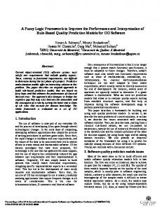
Figure 5. IRIS Mote: An IRIS mote used in our experimental evaluation. The mote has 128 KB of flash, 8 KB of RAM, and it uses an 8-bit AtMega128L processor. It is powered by two AA batteries and is equipped with a 2.4 GHz radio for communication with other motes. free an object that may be reachable but will never be used in future. When an object that is reachable is deallocated by Offline GC then the reference to this object becomes invalid and a subsequent invocation of online GC is likely to report memory errors when it reaches the invalid reference during traversal of the object graph. Our implementation avoids such errors as follows: When an object is deallocated by the OFFLINE GC FREE instruction, the value of the corresponding reference (i.e., the memory location) is stored in a dynamic table. When an online GC traverses the object graph, the value of each encountered reference is first looked up in the dynamic table. If the table contains a reference value, indicating that the memory location pointed to by that reference value has already been freed by Offline GC, the online GC does not dereference that value. The online GC also sets each variable storing such references to null. Thus, at the end of each invocation of online GC, all entries in the dynamic table containing the reference values can be deleted. Memory Overhead: The size of the dynamic table is 2δ bytes (assuming that a reference occupies 2 bytes), where δ is the number of objects that are deallocated by Offline GC since the last invocation of the online GC. The table entries are removed at the completion of each online GC cycle.

6

Results and Discussion

The use of Offline GC offers two main advantages as compared to when only a traditional, online garbage collector is used: (1) additional RAM is made available for a user Java program, and (2) the number of CPU cycles consumed in deallocating objects at runtime is reduced, resulting in an increased battery lifetime of the host device. These advantages come with two drawbacks: (1) the increased flash storage requirement, and (2) a longer compilation time of a program. We first describe the programs used to measure the characteristics of Offline GC.

6.1

Benchmark Programs

We have implemented Offline GC on the TakaTuka JVM [3]. This JVM supports wireless sensor motes which typically have at the most 10 KB of RAM and 128 KB of flash storage. Many existing GC benchmarks, such as SPECjbb2005, SPECjvm2008 and EEMBC [15, 16], or an arbitrary Java program cannot be selected to run on such a resource-constrained device. For our evaluation we needed benchmarks developed for resource constrained sensor motes or are flexible enough to reduce their default memory requirements. We found two such GC benchmarks

Benchmark Name

Brief Description

Evaluation Platform

JTC

JVM Test Cases. Taken from the TakaTuka Sourceforge repository. Includes hundreds of test cases. The test cases are developed to check the Java binary instructions set implementation of a JVM. Designed to mimic memory usage behavior of real applications. Default RAM requirement is 32 MB. To fit the benchmark onto a tiny mote with 4 KB RAM, we used the following input parameters: kStretchTreeDepth=7, kLongLivedTreeDepth=25, kArraySize=100, kMinTreeDepth=4, and kMaxTreeDepth=10. A description of these parameters may be obtained from the source code [12]. The benchmark creates a mix of long and short lived objects. The short lived objects are binary trees. To constrain the memory, we changed the binary tree structure to a linked list. A GC benchmark developed at Sun Microsystems for garbage collection research [12]. It creates binary trees for short and long lived objects. We have changed the following parameters so that it can run on a tiny mote using a few KBs of RAM: MEG=2, INSIGNIFICANT=5, BYTES PER WORD=1, BYTES PER NODE=1, treeHeight=4, size=14, workUnits=20, promoteRate=2, ptrMutRate=5, and steps=20. A description of these parameters may be obtained from the implementation of GCOld [12]. The in-place iterative implementation of the Quicksort algorithm. Each iteration creates very few dynamic objects. This program is selected to show that Offline GC is to be used with caution; it may not be beneficial if a program has only a few dynamic objects. Taken from the TakaTuka sourceforge repository. CTP is an address-free routing protocol for networks that use wireless sensor motes [13]. The protocol is completely implemented using Java and uses four threads. Taken from the TakaTuka sourceforge repository. DYMO is a successor to the Ad hoc On-Demand Distance Vector (AODV) routing protocol [14]. The protocol is completely implemented using Java with threads.

Mica2, Avrora

GCBench

GCOld

QuickSort

CTP

DYMO

Mica2, Avrora

Mica2, Avrora

Mica2, Avrora

IRIS (see Fig. 5)

IRIS

Table 1. Benchmarks used for the evaluation of Offline GC. namely GCBench and GCOld [17, 12] whose RAM requirements were dependent upon their input parameters. In addition to these two benchmarks, we have also used three existing applications from the TakaTuka JVM sourceforge repository. These applications have been developed for the resource constraints of sensor motes. Table 1 provides a description of these five benchmarks, which are used for the evaluation of Offline GC.

6.2

Evaluation Results

This section provides an evaluation of Offline GC on the first four benchmarks in Table 1. We evaluated these benchmark programs on Crossbow Mica2 motes [1, 18] as well as on Avrora which is a simulator for the Mica2 motes [19].

The memory usage results for the actual Mica2 motes and the Avrora simulator were found to be consistent with each other. For measuring the CPU cycles consumed in deallocating the objects, we used only the Avrora simulator because it is hard to measure the CPU cycles on an actual sensor mote. Avrora simulates microcontroller instructions and can accurately calculate the CPU cycles consumed by a set of procedures during the execution of a program. In order to preserve the correlation of memory usage with CPU cycles, both of these results are presented using the Avrora simulator.

6.2.1

RAM Availability

The results for RAM-available at a point of execution with and without the use of Offline GC have been shown

(a) JTC

(b) GCBench

(c) GCOld

Figure 6. RAM-available: The amount of RAM-available in bytes at different points of execution for the first three benchmarks given in Table 1. in Fig. 6. The term RAM-available at a given point of execution refers to the maximum amount of memory that becomes available to a program if a precise compacting online GC is executed at that point. Thus, at every execution point, the actual free memory will always be less than or equal to the RAM-available at that point. Furthermore, if RAM-available at a point is 0 bytes, then a program is deemed to be out of memory. It can no longer continue its execution because even running a GC at that point will not free any additional memory. Fig. 6 shows the RAM-available at different points of execution of the JTC, GCBench, and GCOld benchmarks. The JVM Test Cases (JTC) program consists of many test cases, each executing one after the other. Therefore, many dynamic and independent objects are created during the execution of JTC. It is because of the presence of excessive dynamic and independent objects, that JTC on average has 42.37% additional RAM-available during the program execution if Offline GC is used. The GCBench and GCOld programs have, on average, 81.88% and 32.81% additional RAM available respectively when Offline GC is used. Both of these programs have long-lived objects that are created at the start of their execution but are not used afterwards. As these objects are in-scope (reachable) during almost the entire program execution hence they cannot be freed by the online GC. In contrast, Offline GC deallocates these objects soon after their last use, even when they are still reachable. Furthermore, many short-lived objects are also freed by Offline GC a few bytecode instructions ahead of the execution point when an online GC would free them. However, a short lasting increase in RAM-availability like this is not captured in the RAM-availability graphs of these benchmarks. Finally, Fig. 7 shows that in-place Quicksort performs better when Offline GC is not used. This is because this benchmark creates very few (only three) dynamic objects during each iteration for sorting a subset of the input array. None of these objects can be freed by Offline GC earlier than the execution point when a regular online GC would free them. In this case, the RAM-available is 0.6% smaller if Offline GC is used. This reduction is due to the implementation overhead of Offline GC as explained in Section 5. This overhead is present in all the programs and is visible at the beginning of each graph in Fig. 6. However, for a program

that creates many dynamic objects, this overhead is usually negligible as compared to the additional memory made available by Offline GC. In conclusion, Offline GC is effective in bringing down RAM utilization for programs that create several large dynamic objects, each larger than 4 bytes. Thus, for a given program, Offline GC has to be used with caution.

(a) RAM-Available

(b) CPU Cycles

Figure 7. The RAM-available in bytes at different points of execution and number of CPU cycles consumed in deallocating objects, for the Quicksort program with and without the use of Offline GC.

6.2.2

CPU Cycles

The TakaTuka JVM uses a mark-and-sweep online GC with compaction [5, 20]. Considering that the amount of RAM available on motes is limited, the online GC for TakaTuka is designed to be memory efficient by choosing a

(a) JTC

(b) GCBench

(c) GCOld

Figure 8. CPU Cycles: The number of CPU cycles consumed in deallocating objects during the execution of a program, with and without the use of Offline GC.

Benchmark JVM Test Cases GCBench GCOld QuickSort CTP Root CTP Non-Root DYMO Source DYMO Dest.

with Offline GC 8 16 0 12 27 32 11 13

without 47 44 18 13 53 34 29 13

Table 2. The number of times online GC is called by the benchmark programs, with and without Offline GC. The CTP results are produced with inflated objects’ size while receiving 25 data packets at the Root node. Benchmark JVM Test Cases GCBench GCOld QuickSort

% reduction in CPU cycles 8.17 9.65 4.52 −0.21

Table 3. The overall percentage reduction in the number of CPU cycles with Offline GC.

CTP Root CTP Non-Root DYMO Source DYMO Dest.

Max #objects in RAM 63 57 45 48

Extra with Offline GC Bytes RAM in per object bytes 7 7 × 63 = 441 3 3 × 27 = 171 7 7 × 45 = 315 2 2 × 48 = 96

Table 4. Extra RAM-available at each node for CTP and DYMO with the use of Offline GC (shown in the last column). First column shows the maximum number of reachable objects at any time during the execution of the respective program. Second column shows the differential increase (in bytes) in size of each object with and without Offline GC.

non-recursive implementation with multiple iterations of the heap. During a single invocation, the overall time consumed by the online GC is O(k + b2 ), where b is the number of objects on the heap and k is the current size of all stack-frames. In order to minimize the CPU cycle consumption, the online GC is executed only when it is necessary, i.e., when the RAM is nearly full. By deallocating objects at regular intervals, Offline GC reduces the number of times an online GC needs to be invoked (see Table 2 for comparative results of the benchmarks). This leads to a reduction in the number of CPU cycles consumed when Offline GC is used as shown in Fig. 8 and Table 3. The reduction in the number of CPU cycles needed to free objects is 60.56%, 63.48%, and 94.59% for JTC, GCBench, and GCOld, respectively (Fig. 8). This translates into a reduction of 8.17%, 9.65% and 4.52% in the overall CPU cycles required for JTC, GCBench and GCOld, respectively (Table 3). On the other hand, the Quicksort program takes 0.21% extra CPU cycles when Offline GC is used (Table 3 and Fig. 7). This again is because, in case of inplace Quicksort, very few dynamic objects are created and thus the performance gain of Offline GC does not exceed the overhead associated with maintaining it. This results in an increased CPU cycles consumption due to the overhead associated with the execution of the OFFLINE GC NEW and OFFLINE GC FREE instructions.

6.3

Routing Protocols: CTP and DYMO

This section presents performance results of Offline GC for two popular routing protocols – collection tree protocol (CTP) [13] and Dynamic MANET On-demand Routing Protocol (DYMO) [14]. CTP is a tree-based routing protocol in which a few network nodes advertise themselves as root of the network [13]. Based on such advertisements, each non-root node determines which of its neighbors is either a root or nearer to one of the roots. In steady state operation of CTP, a set of distributed routing trees exists with each such tree comprising a root node and several non-root nodes. CTP is an addressfree protocol in which the data is always transmitted from a non-root towards the nearest root node which is part of the same routing tree. The Java implementation of CTP, available in the TakaTuka Sourceforge repository, has a memory requirement of more than 4 KB. Since Avrora only supports Mica2

simulation with a maximum RAM size of 4 KB, we could not use Avrora as the evaluation platform for benchmarking Offline GC with CTP. Instead, we used IRIS motes (see Fig. 5) equipped with 8 KB of RAM [1]. The Java CTP implementation uses four threads, some of which wait to receive the data or control packets. This implies that the bytecode instructions of the program are not executed in a deterministic order, and thus memory usage results, similar to those in Fig. 6 cannot be produced in this case. Therefore, our evaluation of Offline GC with CTP proceeds as follows. We run the benchmark program repeatedly, incrementing the size of all objects by one byte in each successive run. The goal is to find the maximum possible increase of object size before we reach a point where the program exceeds the RAM of the mote. Table 4 indicates that when Offline GC is used, 441 and 171 additional bytes can be occupied by objects for the root and non-root motes, respectively, as compared to the case when only the online GC is used. This implies that a bigger applications can be developed over CTP if Offline GC is used. Furthermore, it is shown in Table 2 that the use of Offline GC results in a reduction in the number of times the online GC is needed to be invoked, thus saving the CPU cycles and hence increasing the battery life of a wireless sensor mote. Results obtained for DYMO were similar to those for CTP when we used the same experimental procedure. Table 4 indicates that 315 bytes of extra RAM are available when Offline GC is used for a source node in DYMO and 96 extra bytes for a destination node.

6.4

Efficacy and Limitations

The effectiveness of using Offline GC is quite prominent for programs that create many large-sized objects. The use of Offline GC does not come for free. That is, the flash storage requirement is increased and the program will take longer to compile. The increase in flash storage requirement is due to two reasons. First, the size of the Java binary gets inflated due to the insertion of the two new bytecode instructions (OFFLINE GC NEW and OFFLINE GC FREE). Second, the size of the Java interpreter is also increased when it provides the implementation of these two new instructions. Fig. 9 shows that, for the benchmarks we used, the aggregated size of the Java binary and the interpreter increases on the average by 3.63 %. This implies that Offline GC does not not increase the flash storage requirements of a mote significantly and it is feasible to use it on a tiny mote device with limited storage. Fig. 9 also shows the time taken in compilation of a program with the use of Offline GC. Before transferring the code on to a mote, the compilation was carried out on a typical notebook with AMD Athlon II P320 / 2.1 GHz processor and 4 GB of RAM. The maximum compilation time taken by a program to compile with Offline GC was 24.33 seconds and average compilation time was 11.5 second for the given set of program. It included the time taken by both of the first two phases of Offline GC as well as the time for changing the bytecode. We believe that this compilation delay is tolerable given that it results in increasing a program’s execution speed and reducing its RAM consumption.

(a) Flash Size

(b) Compilation Time

Figure 9. Fig. (a) shows the aggregated size of Java binary and interpreter (Flash size). Fig. (b) shows the time taken by various components of Offline GC during the first two phases of program compilation before transferring the code on to a mote.

7

Related Work

The notion of compile-time garbage collection goes back to Barth [21] who proposed a scheme for maintaining reference counts at compile time. This topic has been picked up and improved upon by later researches, e.g., [22, 23]. However, this strand of work differs from our proposal which is targeted at mark-and-sweep GC. Free-me [7] is a static analysis that identifies the objects when they become dead, and inserts code to free them. Unlike Offline GC it is based on flow-insensitive and fieldinsensitive pointer analysis, thus it is suitable mostly for local variables. Furthermore, Free-me puts the main emphasis on reclaiming short-lived objects, whereas our analysis handles the long-lived objects also. Shaham et al. [24] provide a yet more precise analysis for placing free instructions. Their approach can even deallocate an object when it is still reachable; however their analysis is intra-procedural and rather expensive in practice. Agesen el al. [25] have also applied type analysis and liveness analysis, but its application is to shrink the root set for a garbage collector. They do not insert explicit free instructions. The scheme proposed by Cherem et al. [26] is closest to our work as it updates the program bytecode using a flowsensitive and inter-procedural pointer analysis. The main limitation of this scheme is that it allows deallocating only those objects that are not shared by multiple fields or local variables at the function boundaries. Thus it cannot deallocate objects that are saved in multiple variables and used by multiple methods. Offline GC overcomes this limitation by

keeping static and non-static field data structures during the analysis phase. A further area of related work is based on escape analysis [8, 9, 10] which determines whether objects can escape from their defining scope. The main application of escape analysis is to determine which objects can safely be allocated on the runtime stack. This allocation is static and the corresponding deallocation is automatic when the function exits. Besides speeding up the program by avoiding the cost of memory management for non-escaping objects, there is also no need to synchronize on such objects as they stay within a thread. While escape analysis speeds up program execution, it may lead to memory leaks because a stack-allocated object cannot be freed before the function returns. In contrast, a heap-allocated object could be freed as soon as it becomes inaccessible. Thus, escape analysis trades execution speed for space. In contrast, the main goal of Offline GC is to reduce the memory consumption of a program without compromising its execution speed. Offline GC is also related to region-based memory management [27]. Each allocation site gives rise to its own region of memory (identified by a tag, following Jones and Muchnick [28]), which is freed when our analysis determines that all references to this region are dead. As with region analysis, our analysis can also free objects that are still reachable and thus would not be reclaimed yet by garbage collection. Much of the work on regions is based on static analysis [29, 30], but there is also work supporting explicit manual region management [31]. While original work supports region deallocation only in a stack-like manner, the subsequent work supports more fine-grain control over the placement of deallocation.

8

Conclusions

We have designed and presented a software optimization for tiny embedded devices that moves the bulk of Java garbage collection offline. Offline GC brings two benefits: it allows running feature-rich large Java programs and it saves on CPU cycles to run a given program thus extending the battery life of such devices that usually operate on battery power. We have also presented three algorithms to facilitate offline deallocation decisions. These algorithms identify where in the program execution an object, which would be left alone by a traditional garbage collector, may be deallocated. Working independently, these algorithms suit different types of programs. Thus, using one or more of these algorithms, a variety of programs can benefit from the use of Offline GC. We performed an evaluation of Offline GC using many programs including the two well-known GC benchmarks and two popular wireless sensor network routing protocol. Our results indicate that Offline GC can reduce the overall CPU cycles required to run a program up to about 10%, while making up to 82% extra RAM available by deallocating reachable objects that cannot be deallocated by any typical online GC. Offline GC is the most useful for applications which allocate many dynamic objects, each larger than 4 bytes. In contrast, applications which reuse same set of

small-footprint objects do not benefit much. For example, the in-place Quicksort, which reuses the same array to sort all objects and makes few dynamic objects, consumes 0.6% additional RAM with Offline GC due to the memory overhead of its runtime implementation. Thus, while Offline GC benefits most sensor application, we caution against its use when a program has very few dynamic objects. Although Offline GC is primarily developed for resource constrained devices, it is also useful for powerful computers running large applications. The results of RAM availability presented in this paper are independent of the online GC used by a device and the resources available on such a device. It implies that the results presented in Fig. 6 will remain unchanged, if an online GC other than mark-and-sweep is employed on a device with plenty of resources. Furthermore, Offline GC should also scale to large programs developed for powerful computers because each of the three algorithms designed for making the offline deallocation decisions has polynomial time complexity and RAM requirements. Typical programs developed for powerful computers create many large-sized dynamic objects, a situation in which Offline GC is the most beneficial.

9

Acknowledgements

This work is supported in part by the Higher Education Commission (HEC) of Pakistan, the University of Freiburg, and the Max Planck Institute for Software Systems. The authors would like to thank their shepherd John Regehr and the anonymous reviewers for their useful comments.

10

References

[1] ETH Zurich. The Sensor Network Museum. http://www.snm.ethz.ch/Main/HomePage, [Last Accessed: 15.08.2011]. [2] Niels Brouwers, Koen Langendoen, and Peter Corke. Darjeeling, a Feature-Rich VM for the Resource Poor. In Proceedings of the 7th ACM Conference on Embedded Networked Sensor Systems, SenSys ’09, pages 169–182, New York, NY, USA, 2009. ACM. [3] Faisal Aslam, Luminous Fennell, Christian Schindelhauer, Peter Thiemann, Gidon Ernst, Elmar Haussmann, Stefan R¨uhrup, and Zastash Afzal Uzmi. Optimized Java Binary and Virtual Machine for Tiny Motes. In Distributed Computing in Sensor Systems (DCOSS), volume 6131, chapter 2, pages 15–30. Springer Berlin Heidelberg, Berlin, Heidelberg, 2010. [4] Janice J. Heiss. Sentilla’s Pervasive Computing – The Universe Is the Computer. 2008 JavaOne Conference. [5] Richard Jones and Rafael Lins. Garbage Collection: Algorithms for Automatic Dynamic Memory Management. John Wiley & Sons, September 1996. [6] Sigmund Cherem and Radu Rugina. Uniqueness Inference for Compile-Time Object Deallocation. In Proceedings of the 6th international symposium on Memory management, ISMM ’07, pages 117–128, New York, NY, USA, 2007. ACM. [7] Samuel Guyer, Kathryn McKinley, and Daniel Frampton. Free-Me: A Static Analysis for Automatic Individual Object Reclamation. In Proceedings of the 2006 ACM SIGPLAN Conference on Programming Language Design and Implementation, PLDI ’06, pages 364–375, New York, NY, USA, 2006. ACM.

[8] Elvira Albert, Samir Genaim, and Miguel Gomez-Zamalloa. Heap Space Analysis for Java Bytecode. In Proceedings of the 6th International Symposium on Memory Management, ISMM ’07, pages 105–116, New York, NY, USA, 2007. ACM. [9] Jong-Deok Choi, Manish Gupta, Mauricio Serrano, Vugranam C. Sreedhar, and Sam Midkiff. Escape Analysis for Java. In Proceedings of the 14th ACM SIGPLAN Conference on Object-Oriented Programming, Systems, Languages, and Applications, OOPSLA ’99, pages 1–19, New York, NY, USA, 1999. ACM. [10] Bruno Blanchet. Escape Analysis for JavaTM : Theory and Practice. ACM Transactions on Programming Languages and Systems (TOPLAS), 25:713–775, November 2003. [11] Tim Lindholm and Frank Yellin. Java Virtual Machine Specification. Addison-Wesley Longman Publishing Co., Inc., Boston, MA, USA, 2nd edition, 1999. [12] Source code. GCBench and GCOld benchmarks. http://www.cs.cmu.edu/˜spoons/gc/benchmarks.html, [Last Accessed: 15.08.2011]. [13] Omprakash Gnawali, Rodrigo Fonseca, Kyle Jamieson, David Moss, and Philip Levis. Collection Tree Protocol. In Proceedings of the 7th ACM Conference on Embedded Networked Sensor Systems, SenSys ’09, pages 1–14. ACM, 2009. [14] Ian Chakeres and Charles Perkins. Dynamic MANET Ondemand (DYMO) Routing. IETF (work in progress), 2010. [15] David Bacon, Perry Cheng, and David Grove. Garbage Collection for Embedded Systems. In Proceedings of the 4th ACM International Conference on Embedded Software, EMSOFT ’04, pages 125–136, New York, NY, USA, 2004. ACM. [16] Kumar Shiv, Kingsum Chow, Yanping Wang, and Dmitry Petrochenko. SPECjvm2008 Performance Characterization. In Proceedings of the 2009 SPEC Benchmark Workshop on Computer Performance Evaluation and Benchmarking, pages 17–35, Berlin, Heidelberg, 2009. Springer-Verlag. [17] Daniel Spoonhower, Guy Blelloch, and Robert Harper. Using Page Residency to Balance Tradeoffs in Tracing Garbage Collection. In Proceedings of the 1st ACM/USENIX International Conference on Virtual Execution Environments, VEE ’05, pages 57–67, New York, NY, USA, 2005. ACM. [18] Crossbow Technology. Wireless Sensor Networks. http://www.xbow.com, [Last Accessed: 15.02.2011]. [19] Ben Lawrence Titzer, Daniel Lee, and Jens Palsberg. Avrora: Scalable Sensor Network Simulation with Precise Timing. In Proceedings of the 4th International Symposium on Information Processing in Sensor Networks, IPSN ’05, Piscataway, NJ, USA, 2005. IEEE Press. [20] Luminous Fennell. Garbage Collection for TakaTuka, Bachelors Thesis. University of Freiburg, Germany, 2010. [21] Jeffrey Barth. Shifting Garbage Collection Overhead to Com-

[22]

[23]

[24]

[25]

[26]

[27]

[28]

[29]

[30]

[31]

pile Time. Communications of the ACM (CACM), 20:513– 518, July 1977. Pramod Joisha. Overlooking Roots: A Framework for Making Nondeferred Reference-Counting Garbage Collection Fast. In Proceedings of the 6th International Symposium on Memory Management, ISMM ’07, pages 141–158, New York, NY, USA, 2007. ACM. Wolfram Schulte. Deriving Residual Reference Count Garbage Collectors. In Symposium on Programming Language Implementation and Logic Programming (PLILP), pages 102–116. Springer-Verlag, 1994. Ran Shaham, Eran Yahav, Elliot Kolodner, and Mooly Sagiv. Establishing Local Temporal Heap Safety Properties with Applications to Compile-Time Memory Management. In Static Analysis, volume 2694 of Lecture Notes in Computer Science, pages 483–503. Springer Berlin / Heidelberg, 2003. Ole Agesen, David Detlefs, and J. Eliot Moss. Garbage collection and local variable type-precision and liveness in Java virtual machines. In Proceedings of the ACM SIGPLAN 1998 Conference on Programming Language Design and Implementation, PLDI ’98, pages 269–279, New York, NY, USA, 1998. ACM. Sigmund Cherem and Radu Rugina. Compile-Time Deallocation of Individual Objects. In Proceedings of the 5th International Symposium on Memory Management, ISMM ’06, pages 138–149, New York, NY, USA, 2006. ACM. Dan Grossman, Greg Morrisett, Trevor Jim, Michael Hicks, Yanling Wang, and James Cheney. Region-Based Memory Management in Cyclone. In Proceedings of the ACM SIGPLAN 2002 Conference on Programming Language Design and Implementation, PLDI ’02, pages 282–293, New York, NY, USA, 2002. ACM. Neil Jones and Steven Muchnick. Flow Analysis and Optimization of LISP-like Structures. In Proceedings of the 6th ACM SIGACT-SIGPLAN Symposium on Principles of Programming Languages, POPL ’79, pages 244–256, New York, NY, USA, 1979. ACM. Alexandru Stefan, Florin Craciun, and Wei-Ngan Chin. A Flow-Sensitive Region Inference for CLI. In Proceedings of the 6th Asian Symposium on Programming Languages and Systems, APLAS ’08, pages 19–35, Berlin, Heidelberg, 2008. Springer-Verlag. Sigmund Cherem and Radu Rugina. Region Analysis and Transformation for Java Programs. In Proceedings of the 4th International Symposium on Memory Management, ISMM ’04, pages 85–96, New York, NY, USA, 2004. ACM. David Gay and Alex Aiken. Memory Management with Explicit Regions. In Proceedings of the ACM SIGPLAN 1998 Conference on Programming Language Design and Implementation, PLDI ’98, pages 313–323, New York, NY, USA, 1998. ACM.