Mitchell Peabody in partial fulfillment of the ... Mitchell Peabody. All Rights Reserved. ...... [32] George Cybenko, Aditya Bhasin, and Kurt D. Cohen. 3d base: An ...
Finding Groups of Graphs in Databases A Thesis Submitted to the Faculty of Drexel University by Mitchell Peabody in partial fulfillment of the requirements for the degree of Master of Science in Computer Science August 2002
c Copyright 2003 Mitchell Peabody. All Rights Reserved.
ii
Dedications “I love deadlines. I like the whooshing sound they make as they fly by.” — Douglas Adams
This work is dedicated to my mother and father, for their love and encouragement. To my siblings, Natalie, Jason, Karla, and Stephen, for inspiring their oldest brother. Finally, a special thanks goes to Major Eric Schaertl. He was, and is, a wise mentor and role model for me. Over the past four years, his guidance and advice were invaluable in my growth as a student, leader, and man. He has my eternal gratitude.
iii
Acknowledgements I wish to acknowledge Dr. William Regli and Dr. Ali Shokoufandeh, for allowing me to work in GICL. The opportunities and successes that I have had would not have been possible without them. Dr. Spiros Mancoridis, for chairing my thesis committee on such short notice. Craig Schroeder and Matt Maycock for reviewing my thesis at various times and providing numerous suggestions and corrections. This work was supported in part by the Office of Naval Research (ONR) Award No. N00014-01-1-0618 and National Science Foundation (NSF) Award No. CISE/IIS-9733545. Any opinions, findings, conclusions, or recommendations expressed in this material are those of the author and do not necessarily reflect the views of the National Science Foundation or the other supporting government and corporate organizations.
iv
Table of Contents List of Tables . . . . . . . . . . . . . . . . . . . . . . . . . . . . . . . . . . . . .
vii
List of Figures . . . . . . . . . . . . . . . . . . . . . . . . . . . . . . . . . . . . .
viii
Abstract . . . . . . . . . . . . . . . . . . . . . . . . . . . . . . . . . . . . . . . .
x
1 Introduction . . . . . . . . . . . . . . . . . . . . . . . . . . . . . . . . . . . .
1
1.1
Problem . . . . . . . . . . . . . . . . . . . . . . . . . . . . . . . . . . .
1
1.2
What I Do . . . . . . . . . . . . . . . . . . . . . . . . . . . . . . . . . .
3
1.3
Outline of Thesis . . . . . . . . . . . . . . . . . . . . . . . . . . . . . .
4
2 Background . . . . . . . . . . . . . . . . . . . . . . . . . . . . . . . . . . . .
5
2.1
Databases . . . . . . . . . . . . . . . . . . . . . . . . . . . . . . . . . .
5
2.1.1
Relational Paradigm . . . . . . . . . . . . . . . . . . . . . . . .
5
2.1.2
Multimedia Databases . . . . . . . . . . . . . . . . . . . . . . .
6
2.1.3
Querying Databases . . . . . . . . . . . . . . . . . . . . . . . . .
7
Graph Theory . . . . . . . . . . . . . . . . . . . . . . . . . . . . . . . .
8
2.2.1
Isomorphism Problems . . . . . . . . . . . . . . . . . . . . . . .
9
2.2.2
Edit Distance . . . . . . . . . . . . . . . . . . . . . . . . . . . .
9
2.2.3
Maximal Common Subgraph . . . . . . . . . . . . . . . . . . . .
11
2.2.4
Algebraic Graph Theory . . . . . . . . . . . . . . . . . . . . . .
12
2.2.5
Spectral Graph Theory . . . . . . . . . . . . . . . . . . . . . . .
13
2.2.6
Cospectral Graphs . . . . . . . . . . . . . . . . . . . . . . . . .
14
2.2.7
Eigendistance (λ -distance) . . . . . . . . . . . . . . . . . . . . .
14
2.2.8
Graphs in Databases . . . . . . . . . . . . . . . . . . . . . . . .
15
2.3
Metric Spaces . . . . . . . . . . . . . . . . . . . . . . . . . . . . . . . .
16
2.4
Clustering . . . . . . . . . . . . . . . . . . . . . . . . . . . . . . . . . .
17
2.2
v
2.5
Solid Models . . . . . . . . . . . . . . . . . . . . . . . . . . . . . . . .
18
2.5.1
Solid Modeling and Computer-Aided Design . . . . . . . . . . .
18
2.5.2
Engineering Databases . . . . . . . . . . . . . . . . . . . . . . .
20
3 Approach . . . . . . . . . . . . . . . . . . . . . . . . . . . . . . . . . . . . .
22
3.1
Graphs in a Database . . . . . . . . . . . . . . . . . . . . . . . . . . . .
22
3.2
λ -distance . . . . . . . . . . . . . . . . . . . . . . . . . . . . . . . . . .
23
3.2.1
The Ψ Operator . . . . . . . . . . . . . . . . . . . . . . . . . . .
23
3.2.2
The Noise Matrix . . . . . . . . . . . . . . . . . . . . . . . . . .
24
3.2.3
Distortion Bounds . . . . . . . . . . . . . . . . . . . . . . . . . .
24
3.2.4
λ -distance Expressed Using the Ψ-operator . . . . . . . . . . . .
26
3.2.5
Theoretical Bounds on Distance Calculations . . . . . . . . . . .
26
3.2.6
An Example Calculation . . . . . . . . . . . . . . . . . . . . . .
27
Cospectral Non-Isomorphic Graphs . . . . . . . . . . . . . . . . . . . . .
29
3.3.1
Extending λ -Vectors (mλ -Vectors) . . . . . . . . . . . . . . . . .
30
3.3.2
mλ -Distance Calculation . . . . . . . . . . . . . . . . . . . . . .
32
k-Clustering of Graphs . . . . . . . . . . . . . . . . . . . . . . . . . . .
34
3.4.1
Refinement of Initial Points . . . . . . . . . . . . . . . . . . . . .
35
3.4.2
Measurement of Quality . . . . . . . . . . . . . . . . . . . . . .
38
Experiments . . . . . . . . . . . . . . . . . . . . . . . . . . . . . . . . .
40
3.5.1
Stability of λ -Distance and mλ -Distance . . . . . . . . . . . . .
40
3.5.2
Clustering of Synthetic Data . . . . . . . . . . . . . . . . . . . .
41
3.5.3
Clustering Real World Data . . . . . . . . . . . . . . . . . . . . .
43
4 Results and Discussion . . . . . . . . . . . . . . . . . . . . . . . . . . . . . .
48
3.3
3.4
3.5
4.1
Complexity . . . . . . . . . . . . . . . . . . . . . . . . . . . . . . . . .
48
vi
4.1.1
λ -Vector and mλ -Vector Calculation . . . . . . . . . . . . . . . .
48
4.1.2
λ -Vector and mλ -Vector Distance Calculation Timing . . . . . .
48
4.1.3
Complexity of k-means Algorithm . . . . . . . . . . . . . . . . .
50
4.2
Distance Calculations Using λ -Vectors and mλ -Vectors . . . . . . . . . .
53
4.3
Clustering on Synthetic Data . . . . . . . . . . . . . . . . . . . . . . . .
55
4.3.1
Clustering Using Known Seed Points . . . . . . . . . . . . . . .
55
4.3.2
Clustering Using Seed Points from Refinement Algorithm . . . .
58
4.3.3
Clustering of Datasets Using the mλ -Vector . . . . . . . . . . . .
59
Clustering on Real World Data . . . . . . . . . . . . . . . . . . . . . . .
60
4.4.1
Using λ -Vectors on Model Signature Graphs . . . . . . . . . . .
62
4.4.2
Using λ -Vectors on Feature Signature Graphs . . . . . . . . . . .
66
Failed Experiments . . . . . . . . . . . . . . . . . . . . . . . . . . . . .
72
5 Conclusions and Summary . . . . . . . . . . . . . . . . . . . . . . . . . . . .
73
4.4
4.5
5.1
Summary . . . . . . . . . . . . . . . . . . . . . . . . . . . . . . . . . .
73
5.2
Limitations . . . . . . . . . . . . . . . . . . . . . . . . . . . . . . . . .
73
5.3
Directions for Future Work . . . . . . . . . . . . . . . . . . . . . . . . .
74
5.3.1
Query Semantics . . . . . . . . . . . . . . . . . . . . . . . . . .
74
5.3.2
Recent Clustering Algorithm Advances . . . . . . . . . . . . . .
75
5.3.3
Distortions in Projected Dimensionality . . . . . . . . . . . . . .
76
5.3.4
Embedding Graphs in Metric Spaces . . . . . . . . . . . . . . . .
77
5.3.5
mλ -vector Development . . . . . . . . . . . . . . . . . . . . . .
77
Bibliography . . . . . . . . . . . . . . . . . . . . . . . . . . . . . . . . . . . . .
78
vii
List of Tables 2.1
An example relation R . . . . . . . . . . . . . . . . . . . . . . . . . . . .
5
4.1
Results of clustering the datasets using mλ -vector . . . . . . . . . . . . .
60
4.2
Error values for the best clustering found on the MSG dataset . . . . . . .
61
4.3
Error values for the best clustering found on the FSG dataset . . . . . . .
66
4.4
Error values for the best clustering found on the FSG dataset . . . . . . .
71
5.1
Relation R and S with a graph attributes . . . . . . . . . . . . . . . . . .
75
viii
List of Figures
�
G3 . . . .
10
2.2
Topological information in the BRep used by ACIS [90] . . . . . . . . . .
19
3.1
Example graphs . . . . . . . . . . . . . . . . . . . . . . . . . . . . . . .
27
3.2
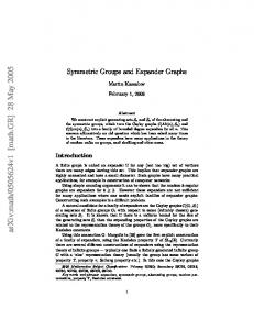
Two cospectral graphs with λ -distance equal to 0. [49] . . . . . . . . . .
29
3.3
Graphs induced by removing each vertex successively . . . . . . . . . . .
31
3.4
Two graphs with the same number of vertices . . . . . . . . . . . . . . .
32
3.5
An
example of controlled clusters of points . . . . . . . . . . . . . . .
42
3.6
Representations of a Torpedo Motor as a wireframe and MSG . . . . . . .
45
3.7
Representations of an Allied Signal part as a wireframe and MSG . . . . .
46
4.1
λ -vector and mλ -vector creation times vs. size of graph . . . . . . . . . .
48
4.2
Distance calculation times vs. size of graph . . . . . . . . . . . . . . . .
49
4.3
Timing of k-means on dataset 1 using the λ -distance function . . . . . . .
50
4.4
Normalized distances of λ and mλ vs. the number of rotations . . . . . .
53
4.5
Cluster error vs. number of cluster on dataset 1 using λ -distance . . . . .
55
4.6
Cluster quality vs. number of clusters on dataset 1 using λ -distance . . .
55
4.7
Cluster quality vs. number of clusters on dataset 1 using VE-vector . . . .
56
4.8
Cluster quality vs. number of clusters on dataset 2 using λ -distance . . .
57
4.9
Cluster quality vs. number of clusters on dataset 2 using VE-vector . . . .
57
4.10 Cluster purity vs. number of clusters on dataset 1 using refine-points . . .
58
4.11 Cluster purity vs. number of clusters on dataset 2 using refine-points . . .
59
4.12 Cluster error vs. number of clusters for the model signature graphs . . . .
61
4.13 Models from cluster22 and their corresponding MSGs . . . . . . . . . . .
63
4.14 Models from cluster17 and their corresponding MSGs . . . . . . . . . . .
64
2
G2
�
Equivalent graphs under the
�
relation. In this case, G1
�
2.1
ix
4.15 Cluster error vs. number of clusters for the feature signature graphs . . . .
65
4.16 Models from cluster0 and their corresponding FSGs . . . . . . . . . . . .
67
4.17 Models from cluster10 and their corresponding FSGs . . . . . . . . . . .
69
4.18 Models from cluster1 and their corresponding FSGs . . . . . . . . . . . .
70
4.19 Models from cluster13 and their corresponding FSGs . . . . . . . . . . .
71
x
Abstract Finding Groups of Graphs in Databases Mitchell Peabody William C. Regli, PhD. and Ali Shokoufandeh, PhD.
Presented with a database of solid models, the task is to group the solid models together by similarity. This similarity can be defined in a number of ways, including topological or feature interaction. It turns out that both of these similarity metrics can be represented by undirected, simple graphs, and the problem can be abtracted to grouping graphs by similarity. To do this, a metric that captures the differences in graphs is needed. Unfortunately, known metrics are NP-Hard to calculate. In this thesis, I further expand on an approximate similarity metric known as λ -distance and propose a way to handle cospectral graphs. In addition, I use a well established clustering algorithm to graphs these graphs into clusters. I use techniques from information theory to measure the quality of results on controlled datasets of random graphs. This work is applied to the problem of grouping a set of solid models.
1 Chapter 1: Introduction
1.1 Problem Computer Aided Design (CAD) enables modern engineers to rapidly conceptualize, prototype, and test parts before physical creation. This ease of creation leads to decreased research and development costs and fewer defects in physical prototypes. The use of CAD has also caused an explosion in the number of models that are stored in company archives. Often indexed in databases according to a manually derived part encoding, an important research question is how to use the intrinsic properties of the models to perform queries based on desired proprties. Consider an engineer that would like to see if a part with a particular topology has already been created. Assuming that a system to index these models exists, the engineer could sketch a conceptual diagram or describe in English the general properties of the model. The system would then check the indexes for parts that satisfy the query and return the results to the engineer. An appropriate part could be selected from the results to be modified for a specific application; instead of being created from scratch by the engineer. The problem of efficiently storing solid models in a database for rapid querying is really a problem of indexing. Indexing records in a database requires a measure of similarity and, for simple primitive datatypes such as integers and strings, these are already wellestablished. Multimedia data presents a special challenge to databases since the notion of similarity often depends on the specific application. One person querying a database of images might be interested in what objects appear in the foreground of the image while another person might be interested to see if there are any images similar to a given query image. A database of solid models is an instance of a multimedia database. A solid model
2 database requires a flexible notion of similarity in the same way as an image database. Two models might be very different topologically and yet require similar machining tools. This thesis addresses the development of the similarity measures required for the creation of solid model databases. The similarity measure for 3D models must be invariant in terms of scale, rotation, translation, and shear; a cube is a cube whether is 2 inches on a side or 5 meters. To model this invariance, the use of a graph representation of a solid model is employed. Graphs have a long history as a powerful and flexible structure for many problems and have proven to be quite useful in the representation of objects in practical domains such as computer vision [25], seal verification [60], 3D object recognition [24], schematic representation [61], handwriting recognition [66], model matching [99, 50], and more. With numerous applications of graph theory, a method of managing this information is desirable. The problem of managing huge amounts of graph data is not a new problem and has been addressed before in numerous ways. In the prevailing paradigm for information management, it makes sense to store graphs in a relational database as described by [29]. A Relational Database Management System (RDBMS) represents data in a logically related fashion with specific semantics for querying this data. Most databases that contain graphs either treat the entire database of relations as a graph, or represent the graph as a group of relations in the database. These representations present problems for query languages. How is the notion of querying the database for a graph regarded? This particular question poses several subproblems that need to be addressed. For instance, what is the nature of the questions that can be asked? How is the result set built up from a query? What is meant by the query, “Find me all the graphs like this one”? Does the user want exact matches or fuzzy matches? How is similarity defined and how can this definition be tested? This formulation requires defining when graphs equal to each other as well as other logi-
3 cal comparisons. As can be seen, the way to solve these questions is not always the most obvious. The simple flexibility in graphs of graphs that give them wonderful representational abilities also bestows upon them the annoying quirk that most of the interesting questions that can be posed about them are NP-Complete or NP-Hard meaning that unless P
�
NP,
there is no hope of solving them in a tractable amount of time. To answer the first question, such measures do exist: edit-distance and maximal-common subgraph, are two proven metrics on graph similarity. They will be discussed later in Sections 2.2.2 and 2.2.3, but they both have the flaw that they are both NP-Hard to compute for the general case. This leads in the direction of an approximation to these metrics, which was proposed and experimented with by McWherter in his thesis [69] on distance based indexing algorithms for graphs. As with all data, finding groups of data, or classifying data into groups based on some similarity measure is also desirable. The process of finding groups within data is known as clustering. Typically, this data consists of points in multidimensional space. In an optimal clustering, points within a group are more similar to points within that group than points in other groups. This process is very time and processor intensive and has been the subject of intense research both for theoretical and practical purposes. In a database of graphs, a good clustering of the graphs should aid in the creation of specialized indexes to speed query time as well as lead to the discovery of previously unknown patterns. 1.2 What I Do I address two subproblems of managing graphs in a database. The first subproblem is to solidify the theoretical underpinnings of the eigen-distance (λ -distance) metric. Although the experiments and measurements performed by McWherter were empirically very interesting and useful, there are some questions that still need to be resolved. I will formalize the
4 notation for eigen-distance measures and provide bounds for the distortions on the eigenvalues caused by edit-operations. I also validate the stability measurements performed by McWherter. In addition, I will address the problem of measuring the distance between two isospectral graphs by developing an extension of the λ -vector structure used by the
λ -distance and show that this distance has the same desirable properties of λ -distance with some added benefits. The second subproblem addressed is that of finding groups of similar graphs in a database setting. To this end, I implement two distance based clustering algorithms using the eigen-distance approximation metric [70, 72, 71]. In order to verify that these clustering methods do indeed group graphs appropriately, I will construct a synthetic data set. The quality of the clustering of this synthetic data will be measured based on the concept of entropy, purity, and total error. I will then turn these clustering methods onto a set of real-world data drawn from the feature graphs and topology graphs of solid models found in the National Design Repository [74] to show a practical application of the clustering methods. 1.3 Outline of Thesis This thesis is broken into four main areas. Chapter 2 briefly discusses research areas relevant to my research as well as previous work by others. Chapter 3 formulates the problem and details the approach taken in my research, rationale, and lays out the experiments conducted. Chapter 4 presents and analyzes the results of the experiments and discusses issues and problems encountered during the course of experimentation. Finally, Chapter 5 discusses what can be concluded from my research and directions for future work.
5 Chapter 2: Background
2.1 Databases 2.1.1 Relational Paradigm The relational paradigm of databases was introduced in [29] and opened up a whole new area of practical research. Prior to Codd’s work, databases were essentially proprietary data structures that imposed no restrictions on how the data was logically organized, manipulated, or queried. The central concept in the relational paradigm is to apply relational algebra to a database system while placing minimal restrictions on the way the data is physically organized. In this approach, a relation R is a set of n-tuples. Given the sets S1 , S2 , . . . , Sn , the first and second elements of each tuple belong to S1 and S2 and so on. Formally, R is a subset of S1
�
S2
���������
Sn . A common representation is in the table format
seen in Table 2.1. When presented in this format, li is said to be a column identifier, and the elements of Si are said to be in the column labeled li . From the relational view, i is the index of the ith column; index i and column identifier li can be used to refer to the elements in Si . Table 2.1: An example relation R. l1 (S1 ) S1 1 S1 2 .. .
l2 (S2 ) S2 1 S2 2 .. .
... ... ... .. .
ln (Sn ) Sn 1 Sn 2 .. .
Relations can be manipulated to provide subsets of data using a few simple operators, which I will now describe briefly. In this thesis, I will use the notation in Ullman et al. [95]; the reader is referred to this book for a deeper discussion of the operators. If R and S are
6 relations with columns labeled l1 , l2 , . . . , ln , then the following operations are defined.
Union R S is a relation containing all tuples in R or (inclusive) in S.
�
Intersection R S is a relation containing all the tuples in R and S. Difference R
S is a relation containing all the tuples that are in R but not in S.
�
Projection πL R is a relation containing the columns specified in the column list L from all the tuples in R
�
Selection σC R is a relation containing all tuples in R that satisfy the logical constraint C. Cartesian Product R Natural Joins R
��
�
S are all the possible pairs of tuples between R and S.
S are the tuples from R and S which are identical for which the at-
tributes match up in some way. Theta Joins R
��
C
S are all the tuples from R and S which satisfy the condition C.
2.1.2 Multimedia Databases Multimedia databases store a wide variety of data types. Jain et al. [48] have developed techniques used to index multimedia image data by using feature vectors containing information such as the color, density, or intensity patterns of the image. Their work has been extended to CAD models by using 3D CAD data to create sets of 3D feature vectors of the image related properties of the solid model. The 3D Base Project [32, 33, 30] at Dartmouth uses an approach to performing similarity assessment on CAD models first renders two models using a voxel-based representation. Invariant features of the shape are identified and used to narrow the model search space. Finally, the difference between selected regions of the voxel model is performed to evaluate the model similarity.
7 These vision-based techniques are highly dependent on pixels, color, texture, and other similar properties of the models. None of them do topological comparisons of models under local deformations of scale, orientation, or other transformations. A technique that has been used to achieve transformation invariance is that of Aspect Graphs. This technique computes the set of topologically distinct projections of a solid model onto a plane, and constructs a graph by adding edges between projections whenever one can be directly transformed into another by rotating the model. It is extremely difficult to compute aspect graphs for arbitrary solid models. Therefore, their use is generally restricted to simpler polyhedral models for which the aspect graph can be efficiently computed. Previous work by Elinson, Nau and Regli [38, 37] as well as by Regli and Cicirello [28] has addressed the need for databases that are able to perform retrieval of models based on CAD/CAM-relevant sematics. Previously developed methods for using design and machining features to create graph-based part signatures. This work, however, did not develop indexing or clustering methods, and part retrieval was performed with a linear search of the model dataset. Other research in this direction includes that of Wysk et al. [91], who developed techniques to compare boundary representations of polyhedral objects. 2.1.3 Querying Databases When the relational paradigm from Section 2.1.1 was introduced, data that was being stored was primarily textual or numeric in nature. With the increased interest and use of the multimedia databases described in Section 2.1.2, methods to query and formally describe a language for accessing the data in the databases have been the subject of intensive research. Traditionally, images or videos in databases have been stored with textual or numeric keys that allow users to enter a textual query. The shortcomings to this approach are that putting multimedia data into a database is currently labor intensive and subjective, since it requires that the data be entered manually by a human. While existing indexing and clustering
8 methods can handle this form of data storage, it is not very practical when there are large amounts of data to store and organize. Moreover, while methods to index and cluster this data have been developed, generic ways of querying the data easily have not. Work in creating query interfaces to multimedia databases have resulted in a number of approaches. Some approaches stay fairly close to the relational paradigm. For instance, Fagin [40] describes a language based around the notion of fuzzy set theory [101, 104]. In classical set theory, an object is either in the set or not; in fuzzy set theory, a fractional
� � �����
number 0 1
is assigned to the object and represents the extent to which the object
fulfills the query. For image retrieval, there are several proposals that attempt to abstract the retrieval of images in human readable terms. For instance, Town et al. [94] have created an ontological based query language which attempts to map semantics to images so that queries such as “Find all the cars with a red color.” can be posed using a logic-like language. Many techniques for dealing with complex datatypes have resulted in extensions to the original relational algebra in order to handle special queries or datatypes. For set types, examples of extensions to relational algebra which enable queries of sets in tuple attributes can be found in [76, 63, 64, 15]. Object oriented databases have been the object of intense research for a uniform datamodel and have resulted in such languages as GEM [102], FAD [8], EXODUS [20], DAPLEX [89], and POSTGRES [83]. For semistructured data; where data is missing, irregular, or the structure not fully understood; there is the Lorel query language [1], which has been used for forming queries on XML documents [34]. Other languages that have been proposed include UnQL [14] and a query language based on ambient logic [19, 18]. 2.2 Graph Theory Graphs are a well-studied data structure in computer science. At the most rudimentary level, a graph is a set of vertices and edges. Each edge in the graph is a connection between
9 two vertices. Vertices and edges might be labeled, and, for some domains, a weight may be assigned to the vertices or to the edges, or to both. A graph is said to be simple if there exists no more than one edge between any pair of vertices and no edges from one vertex to itself. For the purposes of this thesis, I am only interested in simple undirected graphs with no weights or labels.
� V � E � , where V G����� v1 � ����� � vn � is the set of vertices in the graph and, E G ����� e1 � ����� � em � is the set of edges in the graph. An edge, e � E will be denoted with a pair of vertices, u and v, as e � u � v � . A pair of vertices u and v are said to be adjacent if there exists an edge e � E G � such that e � u � v � . Furthermore, in undirected graphs, u � v ��� v� u � . In this thesis, a graph G will be denoted by G
2.2.1 Isomorphism Problems Two important problems in graph theory are isomorphism and subgraph-isomorphism. Two graphs, G and H, are said to be isomorphic (G
�
�
of V G to V H such that e
� u � v��� e �
�!
E G
�� e
H) if there exists some mapping
"#� u"$� v"%�&�
�
E H . A graph G is
� some subset of V H � that preserves adjacency among the vertices in both V G � and V H � .
said to be subgraph-isomorphic to a graph H if there exists some mapping from V G to
The subgraph-isomorphism problem is known to be NP-Complete, while the isomorphism problem is suspected to be NP-Complete [44] although there are algorithms that run in polynomial time for special cases. 2.2.2 Edit Distance The edit distance of two graphs is defined by Chartrand et al. [22] as the minimum cost of a series of edit operations needed to transform one graph into another. This was later shown by Kubicka et al. [59] to be a distance metric for graphs. To define the distance between graphs of arbitrary order and size, Kubicka et al. introduced the
�
relation which
10
(a) G1 .
(b) G2 .
Figure 2.1: Equivalent graphs under the says that if G
�
�
(c) G3 .
relation. In this case, G 1
�
G2
�
G3 .
H, then G and H are equivalent because they differ only in the number of
isolated vertices. An example of what this relation means is shown in Figure 2.1. This is a small point that becomes important later in this thesis. The edit distance itself is defined in Equation 2.1.
� ���
n
�(� � O � (2.1) ' where c ok � is the cost of operation ok , c ok ��) 0, and O is one of the following operad GH
min ∑ c ok ok k 1
tions:
� �
1. Delete Edge: remove an edge i j from G.
� �
2. Add Edge: add an edge i j to G.
� ��* i � k �
3. Rotate Edge: transform an edge i j Note that G
�
H
+
� �,�
d GH
in G.
0. A shorthand notation for denoting a transformation of
G to H through edit operations is G
*
H. Edit distance is problematic in that determining
the cost of edit operations is unsolved [16].
11 2.2.3 Maximal Common Subgraph Another metric that can be used for graph similarity is based on the maximal common
"
"
subgraph. G is said to be a common subgraph of G and H if G is subgraph isomorphic
"
to G and H. G is maximal if there are no other common subgraphs of G and H with more nodes. It was shown by Bunke et al. [16] that the maximal common subgraph can be used as a distance metric. Interpreted in words, Equation 2.2 gives an indication of the percentage that G and H differ from each other.
- mcs G � H � � � 1 max - G - � - H - � d G� H �
(2.2)
It has been shown by Bunke [17] that under a restrictive cost function, edit distance is equivalent to the maximal common subgraph problem, and, by extension, the metric. In fact, if the edit operations are all of uniform cost, the worst case upper bound on the
� �/. 2 n s� [59]. Where n is the number of vertices in the graphs, and s � mcs(G, H). If s � 0 then the worst case lower bound is d G � H �0. 2n. This information can be used to calculate the worst case runtime of calculating the edit distance to be O � 3m � 2n n! � where m is the number of edges in the
edit distance between two graphs G and H is d G H
graphs. Readers should refer to McWherter [69] for details. Equation 2.2 is actually a specialization of the more general form of the maximum common subgraph shown in Equation 2.3.
� ���
d GH
� �
1
� �
� �
mGH M GH
(2.3)
� � the size of the problem. Therefore, in Equation 2.2, m G � H ��� mcs G � H � and M G � H ��� - - - max G � H � . Wallis et al. [97] proposed another metric (2.4) using the same m G � H � but - -324- H - - mcs G � H � - , or the size of the viewing the size of the problem as M G � H �1� G
m G H is a measure of the similarity between G and H while M G H is a measure of
12 union of G and H.
- mcs G � H � d G� H � � � 1 - G -526- H - - mcs G � H �
(2.4)
2.2.4 Algebraic Graph Theory Algebraic graph theory is the study of graphs using techniques from linear algebra. Graph properties, or the graphs themselves, are translated into algebraic form. Algebraic techniques are then used to deduce properties and theorems of graphs. Matrix representations have proven to be a fertile ground for examining the structural properties of many types of graphs. There are a number of matrix representations of graphs and each has slightly different properties in terms of the structure of the graphs they represent. One well known representation is the adjacency matrix (2.5).
9
78
� ��� 8:
AG u v
1
: if u is adjacent to v
0
: otherwise.
>
; B
8
D
G.
(2.8)
�
λs 1 , s is the number of unique eigenvalues, and m λk is the
B
number of times λk occurs as an eigenvalue. An alternative version of the spectrum is to list the eigenvalues out in weakly decreasing order as in λ0
G
λ1
G ����� G
λn
B
1
where
� - G - . It is this latter form that will be used for the remainder of this thesis. I will also use the notation that λ D G �!�IH λ0 D G ��� λ1 D G ��� ����� � λ J G J 1 D G ��K , where λ0 D G � G B λ1 D G � G ����� G λ J G J 1 D , and λk D G � represents the kth largest eigenvalue of D G . B
n
The eigenvalues of the different matrix representations for graphs discussed in Sec-
tion 2.2.4 can be used to make different statements about graphs. For instance, in the Biggs
14 form (2.6), it was shown by Mohar [73] that dG
.
2
LNM 42kO k BB λλ OO LL PP$P�Q ln n 13� R 1
G
1
G
. Where dG
is the diameter of a connected, k-regular graph G. A major difference in the matrix representations is the rate at which changes to the structure of the corresponding graph are reflected in the eigenvalues of the matrices. Can the eigenvalues be used for approximating the known similarity metrics for graphs? 2.2.6 Cospectral Graphs The spectrum of an arbitrary graph is a graph invariant. This means that the graph determines the spectrum, but the spectrum does not determine the graph. If G and H have the same spectrum, but are not isomorphic, then they are said to be cospectral. This property of the Laplacian spectrum of graphs poses a problem which is addressed in Section 3.3. 2.2.7 Eigendistance (λ -distance) In his thesis, McWherter [69] defined the eigendistance in terms of the spectrum of
A
G.
The notion is that a distance function can be defined between the eigenvalues to create a metric space of graphs for which it is possible to make relatively quick computations on the similarity of the graphs. The choice of the normalized Laplacian was motivated by the fact that the largest eigenvalue is bounded by 2 which restricts the bounds of the space. The distance calculation itself is simply the L2 norm of the difference between the two vectors (λ -vectors) produced by the spectra of the graphs being compared. To account for
� �
the different number of eigenvalues in differently sized graphs, a Pad v x function was defined which appended a number of values x to the end of the shorter vector v until the appropriate length was reached for the longer vector. If G and H are two graphs with
- H - - G- �
k then the λ -distance formula becomes
λ -distance
A G �SA H �F�UT λ A H �V
A G ��� x�WT 2
Pad λ
15 2.2.8 Graphs in Databases There are a couple ways that graphs can be discussed with respect to a database setting. One is in which the entire database is an instance of a graph. For example, a relation might consist of the set of vertices keyed with another relation which is the set of edges. The totality of this database is a large graph. This is the technique used in Geographic Information Systems (GIS) databases. Another way that graphs can be used in databases is to consider the graphs to be a primitive type in the database, as an attribute of the set of tuples in a relation. Both ways of considering graphs have special implications and require special treatment, especially with respect to querying. In databases where the database an a graph itself, a few query languages have been developed. For example, Afrati [2] developed extensions to the datalog query language and showed that certain queries about the structure of the database can be expressed such as homeomorphism, path finding, and chainy graphs can be made. G-Log [77] is another language that views the database as a grpah. In G-Log, a database scheme is expressed as directed labeled graph. In this system, there are two types of vertices. Elliptical shaped vertices represent what they term as printable nodes and are atomic values within the database, such as integers and strings. Rectangular vertices represent complex objects, called nonprintable nodes. Formally, these schemes are represented as sets of tuples. Queries are expressed in queries resembling an extended version of datalog, the main difference being the semantics of the language with respect to graphs. It is proved that first order logic rules are equivalent in expressive power to G-Log. GOOD [45], a graph-oriented object database system, takes a similar approach to GLog in the representation of the database as a graph. The syntax is not as well defined, and there are a small number of operations, similar to edit operations that are defined for querying the graphs. The main contribution of the paper is the demonstration of a tool for “drawing” queries and constructing database schemas through the use of a graphical sketch
16 tool. Sheng et al. [88] take an object oriented approach in their implementation of a graph query language, called the Graph Object Query Language (GOQL), and modify the Object Query Language (OQL) [21]. In the case of GOQL, the database is not an instance of a graph, and multiple graphs can exist in the database. The graphs themselves are not actually primitive datatypes but a set of relations. One relation contains the graph identifiers, another contains the nodes, and another contains the edges between the nodes. Various types of object definitions are used to represent the sets of nodes and edges in a graph container class. In addition, the query language is extended to deal with the complex datatypes and define functions to support queries about paths and adjacency queries. 2.3 Metric Spaces
� �
Metric spaces are collections of data along with a function, δ x y , known as a distance metric, which computes an effective distance between any two objects in the set. This distance function must satisfy the following conditions:
� �X�
YZ+ x � y δ x � y� G 0 δ x � y �F� δ y� x � 2 δ x � y � δ y� z � G δ x � z � δ xy
0
:
Identity
:
Positivity
:
Symmetry
:
Triangle Equality
Many data types, such as graphs, that do not fit well into a vector space, are easily representable in a metric space. Another significant application of metric spaces are for data sets that have a human-driven interpretation of similarity. Frequently, complex functions can be constructed to approximate the human interpretation of similarity between two or more objects. As long as the measurement satisfies the requirements for a distance metric, or almost achieves them, such a measure can be used to index the data in a way that may be
17 intuitive for a human user. Vector spaces, when used in conjunction with a distance metric such as Euclidean distance, constitute a metric space. 2.4 Clustering Agrawal et al. [4] describes clustering as “...task that seeks to identify homogeneous groups of objects based on the values of their attributes (dimensions)...” Stated more formally, given a set of data points S clusters C
���
d,
a partitioning of this data is defined as a set of
�[� c1 � c2 � ����� � cn � , where a point in a particular cluster ci is more similar to the
points in that cluster than in any other cluster by some similarity function. Algorithms that perform these clusterings have been studied extensively in several different fields such as biology, chemistry, and sociology. There is a large taxonomy of clustering techniques that are all suited for different purposes. Two of the most general techniques are hierarchical and partitional. Fasulo [41] describes a popular and well-studied class of partitional clustering algorithms called k-clustering, which seeks to optimize some objective function over the aggregate whole of the partition. k-clustering takes a set of data points, and attempts to work from the top down. It does this by partitioning the set into disjoint clusters C
] � �
such that ci c j
C, ci
�
cj
�
�\� c1 � c2 � ����� � ck � ,
0/ and some measure of the partition is minimized. The
problem is formally defined in Sahni et al. [84] and shown to be NP-Complete in the general case [43] the datapoints are vertices in a complete graph with non-negative weights. Depending on the measure of quality used, the algorithm might admit a polynomial time approximate solution (PTAS) [7]. Some measures in use are the k-means algorithm [67], k-medioid [58], and an algorithm which minimizes the maximum inter-cluster distance [47]. Weaknesses in these methods that make them inappropriate in a practical setting [41]. They favor spherical clusters, are highly sensitive to outliers, are dependent on the order of the input, are dependent on the
18 initial seeds of the clusters, require the number of clusters be specified in advance, and tend to exhibit expensive run-time properties. In spite of these weaknesses, k-clustering algorithms are still popular because of their ease in implementation. There are workarounds and remedies for almost all the shortcomings, and techniques to address them have been developed by [13, 78, 82, 35, 39]. [4, 3, 23] take unique approaches from most other techniques in that they consider the clusterings that result from different subspaces and groups points together using the best result from a particular subspace. Clustering graphs has generally meant grouping tightly connected nodes together in a single graph for analysis. Graph clustering techniques are used by [54, 53] to improve the query performance of path queries in digital map databases. 2.5 Solid Models 2.5.1 Solid Modeling and Computer-Aided Design There are three broad schemes for the representation of solid models [68, 81]: 1. Decomposition approaches model a solid as collections of connected primitive objects. Data structures used in this type of representation include quad-trees and octtrees [85]. 2. Constructive approaches model a solid as a combination of primitive solid objects. A common approach is constructive solid geometry (CSG), which represents a solid as a boolean expression on a set of primitive solids. 3. Boundary-based approaches model a solid using a data structure that represents the geometry and topology of its bounding faces. Recently, the boundary-representation (BRep) approach has become the representation of choice in solid modeling in large part due to the flexibility and power made available to developers.
19
ENTITY
Topology
BODY
Geometry
SHELL
LUMP
FACE
SUBSHELL
COEDGE LOOP
VERTEX EDGE
CURVE WIRE
POINT
SURFACE PCURVE
ELLIPSE STRAIGHT
INTCURVE
TRANSFORM
SPHERE
CONE
PLANE
SPLINE
TORUS
Figure 2.2: Topological information in the BRep used by ACIS [90]. A BRep solid model creates a unique and unambiguous representation of the exact shape of an object. BReps have become the dominant representation schema for modern solid modelers used in mechanical design. They are used for engineering analysis, simulation, collision detection, animation and manufacturing planning. A BRep usually consists of a graphical structure that models an entity’s topology. Connections between nodes in the BRep graph represent connections between topological components of the entity’s boundary. These topology nodes contain references to their underlying geometric entities. For example, a face of a solid is a topological entity (represented as a collection of bounding edges) that has a surface associated with it. Figure 2.2 shows the distinction between geometric and topological information from the ACIS Solid Modeling Kernel. For more information on boundary representation data structures, interested readers are referred to [51, 68, 98, 100]. BReps and other CAD representations are distinctly different from shape models developed by the computer vision community in several important ways. Vision-based representations, such as super-quadric and deformable shape models, are not designed for exact modeling of shapes; rather they are employed to reconstruct shapes based on approximate data taken from sensors and cameras. These approximated shapes can be used for a basis of comparison among 3D objects, however such comparisons are limited to analysis of ge-
20 ometric moments and gross shape properties. Hence, they are not directly suitable for use in answering the kinds of interrogations that design and manufacturing engineers wish to pose about CAD models. 2.5.2 Engineering Databases In 2D shape matching and image retrieval, the indexing and query process follows one of four common approaches: 1. A textual query based on keywords stored for each image in a database. 2. A query by example uses similarity measures derived off a set of query images provided as input. 3. Query by sketch looks for image segments matching the sketched profile. 4. Iconic queries use templates representing important aspects of the desired image to identify images with similar features. Techniques from computer vision and 2D image retrieval do not directly apply to 3D solid models for several reasons. I will address the three main ones. First, when using solid models involves dealing with an explicit and exact representation of the 3D objects in CAD databases, rather than an approximate representation generated from sensor data.
"
Second, given a solid model A, minor perturbations in A which create A , can make A
"
indistinguishable from A, even though they are still very similar. Transformations such as scaling or rotation can introduce roundoff errors that exacerbate the problems posed by the inexact nature of floating point arithmetic. A simple translation of a model in 3D space by a fixed vector can make models computationally costly to compare. Finally, there is no universally acceptable set of features on which model comparisons can be based. Evaluation metrics for solid models depend on the application intent of the
21 engineers using the database. Process engineers may need to query based on manufacturing process features but an industrial designer may need to consider shape aspects of an object. The ill-defined semantics of the engineering design and manufacturing domain require us create a more flexible methodology for model comparisons which can be customized to consider the criteria of required by different end users.
22 Chapter 3: Approach
3.1 Graphs in a Database I will now define how I will consider graphs in a database. A large part of the focus of our research has been on methods to capture information contained in graphs in databases. The precise definition of what this database will look like is now given in terms of relational databases. As was described before, graph databases generally have two formulations, in one formulation, the entire database is a graph, and in the second, many graphs are stored in the database. It is with the latter approach that this thesis is concerned. For the remainder of this thesis, the reader should consider a database where Ri
acb 1 nd
^_�`� R1 � R2 � ����� � Rn �
are relations in the database. Each relation is a set of tuples; a tuple is a set
of attributes. In the tuples, an attribute can have the tradiftional types (integers, floats, numeric, char, etc) or a graph type. The following are techniques that are being researched with respect to graphs in a database setting. Similarity Assessment Given two graphs G and H, develop a function (or functions)
� �
δ G H that provides a measure of the similarity of G and H. Indexing Given a query request, arrange a database in such a way as to enable rapid searches to fulfill the request. Clustering Given
^
, group the graphs together based on similarity to improve indexing
results and queries time. Querying Given
^
, define the semantics for treating graphs in a relational setting.
This thesis addresses the first and the third topics. McWherter addressed the first and the second topics in his thesis [69]. The fourth problem will be addressed in future work, Section 5.3.
23 3.2 λ -distance While McWherter’s research concentrated on the normalized Laplacian (
A
-matrix)
matrix of a graph, I concentrated on the Laplacian (L -matrix). His reasoning for choosing the
A
� � �
-matrix was that all of the λ ’s are normalized in the interval 0 2 [27], providing
for relatively easy to compute bounds. The L -matrix representation also exhibits some properties that allow it to be bounded, especially in the distance calculation. In order to establish the suitability of λ -distance as an approximate measure of editdistance, I first define how to model any change to a graph can be modeled as a two-step transformation using matrix representations. The first step of the transformation is to make the graph’s original Laplacian matrix into a new matrix that has the same spectral properties as the original matrix. The next step is to add a Laplacian noise matrix that represents the structural changes of this graph. 3.2.1 The Ψ Operator Definition 1 Let G be a graph with m vertices. LG is the m
�
�
m Laplacian matrix of G.
Ψl LG is a lifting operator (projecting operator) which transforms a subspace of a subspace of
� O mf l P e O mf l P , with l G
� m e m to
0.
This transformation takes two steps. In the first step, l zero rows and columns are
g
g
added to LG . Denote this resulting matrix as LG . In the second step, LG is pre- and postmultiplied by a permutation matrix P and its transpose PT , respectively. The resulting
�
g
matrix is denoted Ψl LG . This aligns the rows and columns of LG with the corresponding
�
vertices of both LH and Ψl LG . This operator is spectrum preserving if the eigenvalues
�
of the matrix, LG , and its image with respect to the operator Ψl LG are the same up to a
�
degeneracy. The only difference between the spectrum of LG and Ψl LG is the number of
�
zero eigenvalues (Ψl LG has l more zero eigenvalues than LG ). This operator is an analog
24
"
to the act of adding isolated vertices to a graph, G. Also, if we denote G as the graph
�
represented by Ψl LG , then the relation, G
�
"
G holds.
This is further confirmed by the fact that the number of 0 eigenvalues in the spectrum of G corresponds to the number of connected components of G. [11] Note that by introducing this Ψ operator, the need for the Pad function in the calculation of λ -distance is eliminated. 3.2.2 The Noise Matrix Denote a graph on m vertices by G. Now, assume that a graph H is an n-vertex (where n
G
m) graph obtained by adding n
m vertices and a set of edges to G. These additions to
a graph can be represented by a noise matrix which will be denoted by an n The transformation G
*
H can be written as LH
�
LG
g
2
EH
�
Ψn
B LG � m
� 2
n matrix E H . EH . EH can
be viewed as a matrix description of the operations that are required to transform G into H. This gives us the means to bound the distortions on the eigenvalues induced by the noise matrix EH . 3.2.3 Distortion Bounds Now that the Ψ operator and the noise matrix E have been defined, the impact of the
�h� 1 � �%�i� � n � denote the kth largest eigenvalue of the matrix LGg , then Golub [46] shows that, since LGg , EH , and 2 LGg EH are n � n symmetric matrices, then the following holds: noise on the original graph’s eigenvalues can be quantified. Let λ k for k
2 �
g
λk LG
��.
λn E H
g
λk LG
2
EH
��.
2 �
g
λk LG
�(�
λ1 E H
(3.1)
�j� 1 � �i�i� � n � . For H the perturbed graph and G the original graph, from Equation 3.1 it follows that, for all k �h� 1 � �%�i� � n � : for all k
25
2
g� λn EH ��. - λ L �# k H
2
1� . λk LH �1. λk LGg � λ1 EH �k (3.2) λk LH �V λk LGg �1. λ1 EH � - λk LGg � . max � λ1 EH � � λn EH � � � and since it is already known that λ1 EH � is the largest eigenvalue, λ1 EH � �UT EH T 2 λk LG
λn E H
the spectral radius of EH , then
-λ
k
LH �#
-. TE T
g� \ H 2�
(3.3)
λk LG
The above chain of inequalities gives a precise bound on the distortion of the eigenval-
�
ues of Ψ LG in terms of the largest eigenvalue, or spectral radius, of the noise matrix E H . Since Ψ is a spectrum preserving operator, the eigenvalues of LG follow the same bound in their distortions. This result has important consequences for our application of a graph’s Laplacian eigenvalues to eigen-distance. Namely, if the perturbation matrix EH is small in terms of its complexity, then the eigenvalues of the new graph H (e.g., the query graph) will remain close to their corresponding non-zero eigenvalues of the original graph G, independent of where the perturbation is applied to G. Furthermore, this result holds for any symmetric, real-valued square matrix representation of a graph. Adjacency Matrix Distortions In the case of the adjacency matrix, more precise statements about the perturbation in the eigenvalues can be stated, given specific conditions. If EH is orthogonal to ΨAG then the effect is to add a number of vertices not connected to G. The distortion can then be modeled as a function of the number of vertices added to the graph.
l
For example, if the noise matrix EH introduces new vertices to G in the form of a star graph, then the distortion of every eigenvalue can be bounded by
m l� 1 S� l&)
1 [75]. This
26 bound can be further tightened if the noise matrix has a simple structure. For example, if E H
l
represents a simple path on vertices, then its norm is bounded by 2 cos π
n l 2 1�� �
[65].
3.2.4 λ -distance Expressed Using the Ψ-operator Using the definitions in Section 3.2.1, the definition of λ -distance between the λ vectors of two graph Laplacians can be formally defined as
T �V λ Ψ J H J B J G J LG ���WT 2.
Definition 2 λ -distance(LG , LH ) = λ LH
A similar form can be used for McWherter’s definition: Definition 3 λ -distance(
A
G,
A
H)
T A H �V λ Ψ J H J B J G J A G ���WT 2,
= λ
definition 2 is generalizable to any symmetric, real-valued, matrix representation of graphs, such that the bounds stated in Section 3.2.3 hold. 3.2.5 Theoretical Bounds on Distance Calculations For the case of the Laplacian matrix, a bound on the magnitude of the can be computed as square root of the sum of the maximum theoretical distortion of each of the eigenvalues
δmax
�oT EH T 2 �pT LH
be stated:
0
.
J J B J G J LG �WT 2. Let m � - H - , this allows the following bound to
ΨH
λ -distance(LG , LH )
.
m
2 �rq ∑ δmax
'
i 0
2 mδmax
�
m
δmax m
(3.4)
If the matrices in question are adjacency matrices with an orthogonal noise matrix, then the bound can become even tighter:
0
.
λ -distance(LG , LH )
.\q - G - 2 - H -i- G - - H - , - H - ) - G -
(3.5)
27
(a) Graph G.
(b) Graph H.
Figure 3.1: Example graphs. 3.2.6 An Example Calculation Now an example of the λ -distance computation will be shown I walk through the calculation of λ -distance for the two graphs shown in Figure 3.1. First, the Laplacian matrices LG and LH of G and H are calculated:
stt tt tt
LG
tt
� ttt u
3
0
0
1
1
0
1
0
1
1
1
1
1
3 1 0
0 1 2 0
vxww
1 ww w 0 ww ww 0 ww 0 y 1
28
stt tt
5
tt
tt tt tt
LH
1
1
1
2
0
0
1
0
3
0
t 1 0 0 2 � ttt tt 1 0 1 0 tt 1 0 1 1 t 0 1 0 0 u 0
0
0
1
0
1
0
1
1
0
0
0 1 0
0
1
0
0
0
0
0
4
0
0
0
1
1
0
ww ww ww
0
1
3
1
0
v ww ww ww ww ww
1 ww 1 www 0 y 2
Then, the eigenvalue spectra are calculated:
λG λH clear
�
� 4 � 30278 � 3 � 61803 � 1 � 38197 � 0 � 697224 � 0 � � � � 6 � 23389 � 5 � 21731 � 3 � 64732 � 2 � 59172 � 2 � 25408 � 1 � 62136 � 0 � 434311 � 0 � �
The vectors can then be constructed; since G has fewer eigenvalues the end of the vector
- -
is padded with 0s until the length equals H .
" �
� 4 � 30278 � 3 � 61803 � 1 � 38197 � 0 � 697224 � 0 � 0 � 0 � 0 � � λH � � 6 � 23389 � 5 � 21731 � 3 � 64732 � 2 � 59172 � 2 � 25408 � 1 � 62136 � 0 � 434311 � 0 � � Finally, the λ -distance is calculated using T λG" λH T 2 and is 4 � 78603. The noise matrix is λG" λH and the spectral radius is 5 � 2101 which experimentally confirms the bound on λG
the eigenvalue distortion.
29
(a) J
� � λ LH �z� λ LJ
(b) H
� 6 � 034 � 5 � 963 � 5 � 236 � 5 � 236 � 3 � 588 � 3 � 414 � 3 � 183 � 2 � 279 � 2 � 1 � 757 � 0 � 763 � 0 � 763 � 0 � 691 � 0 � 585 � 0 � 502 � 0 � � 6 034 5 � � � � 963 � 5 � 236 � 5 � 236 � 3 � 588 � 3 � 414 � 3 � 183 � 2 � 279 � 2 � 1 � 757 � 0 � 763 � 0 � 763 � 0 � 691 � 0 � 585 � 0 � 502 � 0 � �
Figure 3.2: Two cospectral graphs with λ -distance equal to 0. [49] 3.3 Cospectral Non-Isomorphic Graphs A problem with the λ -distance metric is that it does not take into account the fact that two graphs can be cospectral. Let the probability that two isospectral graphs G and H with equal number of vertices and edges are not isomorphic will be denoted by
�?
PG
-
�F�
H λ LG
���
λ LH
(3.6)
This probability is not as small as it seems; in fact, it was shown in [86] and generalized in [12] that almost every tree is cospectral with another tree. That result has not been shown for arbitrary graphs, although as Figure 3.2 shows, it is a possibility. Indeed, Halbeisen et al. [49] developed a discrete version of Sunada’s Theorem [92] of isospectral manifolds which they used to generate isospectral, non-isomorphic graphs. This would seem to invalidate the use of the spectrum of the graphs for approximating edit distance; however, consider that what makes the graphs non-isomorphic is some,
30 possibly small, substructure in the graph. This information could be captured by slightly perturbing the graph by inducing a subgraph through the removal of a vertex and the incident edges. Denote the removal of vertex v from G
� V� E �
as Gv
�
n
G v; do this for every v j
�
V . What is generated is a set of spectra for all of the subgraphs induced by removing a single vertex form the graph. If the events of the induced subgraphs are considered to be independent events, then the probability of all the spectra being equal in a n node graph is approximately
{
�� � λ LH ��� P Gv � ? Hv λ LG �F� λ LH ���}|�|�| P Gv ~ � ? Hv ~ λ LG �F� λ LH ��� ~ ~ n 1 � P G � ? H λ LG ��� λ LH ��� ∏i' B 0 P Gv � ? Hv - λ LG �F� λ LH ��� �
�?
PG
-
H λ LG
n 1
n 1
0
vn 1
0
v0
v0
(3.7)
vn 1
i
i
vi
vi
As the number of nodes in the graph increases, this probability approaches 0. This also means that if G and H have the same spectra for each induced subgraph, then the probability that the graphs are isomorphic becomes very large and in fact is 1
{
.
Note that this fact does not invalidate the metric for graphs with different numbers of vertices, since there is already shown a bound in the distortion of the eigenvalues. This means that graphs with the same number of vertices introduces a complication that needs to be accounted for since the λ -distance for isospectral graphs is 0, when in reality, there are a number of edge rotations between the graphs that should be reflected in the metric. 3.3.1 Extending λ -Vectors (mλ -Vectors) While the possibility that non-isomorphic graphs are cospectral can not be eliminated, by using the set of spectra of induced subgraphs it can be made a very remote one. The act of removing each vertex introduces a concept of locality into the notion of the λ -vectors.
31
(a) G.
(d) G v2 .
(b) G v0 .
(c) G v1 .
(f) G v4 .
(e) G v3 .
Figure 3.3: Graphs induced by removing each vertex successively. The perturbation caused by each vertex removal disturbs the eigenvalues in accordance with the local connectivity in the graph.
"
Algorithmically, for a given graph G, induce a subgraph G by iteratively removing each
- -2 1 λ -vectors is
g� the mλ -vector and will be denoted as mλ LG � . The mλ -vector of Figure 3.3a is shown in
vertex from the original G and calculating λ LG . The resulting set of G
Equation 3.8 . An mλ -vector is a set of λ -vectors. The first λ -vector in the set corresponds to the spectrum of the entire graph. Subsequent λ -vectors correspond to the spectrum of the subgraph induced by removing each vertex in turn (the order of removal is not significant).
32
(a) G.
(b) H.
Figure 3.4: Two graphs with the same number of vertices.
stt tt
� � tt tt λ LGC v �� tt λ L �� tt GC v tt λ LGC v �� u λ LGC v �� λ LG C v �� λ LG
0 1 2 3 4
� 4 � 30278 � 3 � 61803 � 1 � 38197 � 0 � 697224 � 0 � � 3� 1� 0� 0� � � 4� 3� 1� 0� � � 3� 1� 0� 0� � � 3 � 41421 � 2 � 0 � 585786 � 0 � � � 4� 3� 1� 0�
v ww
� ww ww ww ww ww ww
(3.8)
y
Referring to the graphs shown in Figure 3.2. Although they are cospectral, by calculating the mλ -vectors for both graphs, it can be seen that there is a difference in the mλ -vectors of the induced subgraphs of J and H. This indicates that it is possible that the mλ -vectors can be used in a more quantifiable manner to determine similarity. 3.3.2 mλ -Distance Calculation The question now is how to calculate the distance using the mλ -vectors? That is, given the two graphs shown in Figure 3.4, what is an appropriate measurement of similarity using mλ -vectors? According to the edit -distance metric, this is the number of edge rotations.
33 If the mλ -vector captures the local information about the topology of the graph, then it is reasonable that the sum of the λ -distances between the corresponding λ -vectors of the two graphs will approximately capture this information. The problem is there is not a well -defined pairing of corresponding λ -vectors. A solution to this is to pair the λ -vector in one mλ -vector with the closest λ -vector in the other mλ -vector in a greedy fashion. An algorithm to get the pairs of eigenvalues is given in Algorithm 2. An algorithm to calculate this distance is given Algorithm 1. In the case of mλ -vectors, the question of what to do when the graphs (and hence the mλ -vectors) are of different sizes. For the λ -vector calculation, Ψ operator had the
�
effect that the
relation defined in [59]. Can this be done for mλ -vectors? Consider the
�
graphs shown in Figure 3.1. When the λ -distance was calculated, λ L G was padded with 0
J J B J G J LG � ). In terms of edit distance, isolated vertices where simply added to G which made the resulting graph equivalent to G under the � relation and (strictly speaking this was Ψ H
produced a corresponding number of 0 eigenvalues. The same effect can be seen if what happens to the mλ -vector when isolated vertices are added to G is considered; such as adding 1 isolated vertex v to G. Each λ -vector is padded with an additional 0 eigenvalue at the end, and a new λ -vector is appended to the
v � . This additional λ -vector corresponds to what the spectrum
set of λ -vectors in mλ LG
Algorithm 1 Distance calculation for mλ -distance. mλ -distance(meig1, meig2) meig1 — a mλ -vector. meig2 — a mλ -vector. 1: ret-distance 0 2: Pad the shorter of meig1 and meig2 to be equal to the longer 3: pairs getPairs(meig1, meig2) 4: for all pair pairs do 5: ret-distance ret-distance pair distance 6: end for 7: return ret distance
�
2
�
34 Algorithm 2 Pairing of λ -vectors for two mλ -vectors. getPairs(meig1, meig2, pairs) meig1 — a mλ -vector. meig2 — a mλ -vector. meig2 meig1 pairs — a vector of size meig1 that contains the λ -vector pairs. 1: used1, used2 — boolean arrays of size meig1 and meig2 initialized to false 2: distances — priority queue of pairs and distances such that smallest distance is on top. 3: used1 0 true, used2 0 true 4: for all λ1 meig1 do 5: for all λ2 meig2 do 6: pq-push(distances, pair-distance(λ1 , λ2 , λ -distance(λ1 , λ2 ))) 7: end for 8: end for 9: while distances 0/ do 10: pair pq-top(distances) 11: if used1 pair λ1 f alse && used2 pair λ2 f alse then 12: vector-push(pairs, pq-top(distances)) true 13: used1 λ1 14: used2 λ2 true 15: end if 16: pq-pop(distances) 17: end while 18: return pairs
-
� �c�
-� -
-
-
-
-
-
-
�
� ��
�
�?
�
� � � �
� �c�
�
�
� �c��
of G v looks like when v is removed. Thus, the analogous Pad function for projecting G
�
�
to be compared to H is to add the appropriate number of λ G to mλ G . The distance calculation in Algorithm 1 can then be run. 3.4 k-Clustering of Graphs k-clustering was intended to cluster points in a vector space with a fixed dimensionality. This poses a slight problem for using the eigendistance metric. The λ -distance does not
� ���
define a true metric space as it violates the condition that δ x y using the equivalence relation
�
0
Y+
x
�
y. However,
between two graphs as defined in [59], the argument can
be made that the identity criteria for a distance function does not need to be strictly applied in approximating the edit-distance precisely because of the
�
relation, the graphs shown
35 in Figure 2.1 are at an edit-distance of 0. Still, the problem of cospectral non-isomorphic graphs is left open. Clustering using mλ -vectors should remedy this. It is clear that under the definition of eigendistance, the dimension of the λ -vectors and mλ -vectors is unbounded in the general case of the entire universe of graphs. For a finite dataset, the dimension of all the comparisons between the λ -vectors and mλ -vectors is eventually projected up into the dth dimension where d is the size of the largest graph in the dataset. Using this fact k-clustering can be adapted to use this metric and definition of λ -vector and mλ -vector, although a much more thorough analysis on the effects of clustering with non-uniform vectors should be done. There has also been some recent research into the distortion caused by projection of metric spaces into lower dimensions which is discussed in Chapter 5. 3.4.1 Refinement of Initial Points The algorithm for k-means is very straightforward and works on the principle that the centers of the clusters will move to the true centers of the data that is being clustered as the algorithm proceeds with its optimization. One of the issues with k-means alluded to in Section 2.4 was the algorithm is highly dependent on the initial point conditions. An algorithm presented in [13, 42] (and reproduced in Algorithm 6) attempts to find the correct initial starting conditions for a distribution for a given number of clusters. The algorithm works on the idea that drawing several small subsamples of the entire dataset will produce cluster centers that are close to the ideal cluster centers. It works in two stages, in the first stage, the algorithm draws j
)
0 subsamples from the population where each
subsample is a certain percentage. It clusters these subsamples using k-means for a given size of k. It then takes the cluster centers and places them into a set. In the next stage, the set of cluster centers is repeatedly clustered as its own dataset using each subset of centers as the initial starting condition. The set that produces the lowest square error in the final
36 Algorithm 3 k-means algorithm. k-means(k, S, D, δ , o) k — an integer that specifies the number of clusters to make. S — set of k starting points. D — set of points to be placed into k clusters. δ — distance function for points. o — cutoff value for optimization loops. 1: C C1 C2 Ck 2: WeightedError 0 3: for i 1 to k do 4: Ci Si 5: Rep(Ci ) Si 6: end for 7: for all D j D do 8: minC i, such that δ (Rep(Ci ), D j ) is minimized. 9: CminC CminC Dj 10: end for 11: for i 1 to k do 12: Rep(Ci ) RepFunction(Ci ) 13: end for 1 14: iteration 15: while No Improvement in WeightedError && iteration o do 16: for all D j D do 17: Remove D j from the cluster it is currently in. 18: minC i, such that δ (Rep(Ci ), D j ) is minimized. 19: CminC CminC Dj 20: end for 21: TotalError 0 22: for i 1 to k do 23: Rep(Ci ) RepFunction(Ci ) 24: ClusterError ErrorFunction(Ci , Rep(Ci )) Ci D k 25: ClusterWeight 26: TotalError TotalError ClusterWeight ClusterError 27: end for 28: iteration iteration 1 29: end while 30: Remove all 0 sized clusters. 31: Return C
� � � �� ��� � � � � � �
Z� � � �
Z� � � - - - -2 n 2 � 2
.
partition has its cluster centers used for the initial starting conditions for clustering on the entire dataset.
37 Algorithm 4 Representative function. RepFunction(C) C — A cluster to get the representative of. 1: MaxDimension 0 2: for all Points p C do 3: if p dimension MaxDimension then 4: MaxDimension p dimension 5: end if 6: end for 7: Construct a point SumPoint in MaxDimension-dimensional space centered at origin 8: for all Points p C do 9: for i 0 to p dimension do 10: SumPointi SumPointi pi 11: end for 12: end for 13: for i 0 to SumPoint dimension do 14: SumPointi SumPointi C 15: end for 16: Return SumPoint
�
G
�
�
�
�
�
�
�
2
n- -
My implementation differs slightly from that given by Bradley et al [13] in that clusters with a size of 0 are not reseeded with the furthest point and reclustered. My implementation simply prunes the 0 size clusters from the partition. This modification was made with the realization that there will be a large number of points in the dataset which overlap due to isospectral properties and possibly isomorphic graphs. For instance, the National Design Repository, from which the real world test-data is drawn, has a large number of models with the same spectrum due to minute changes not captured in the graphs. Algorithm 5 Error function. ErrorFunction(C) C — A cluster to get the error of. 1: ErrorSum 0 2: for all p C do 3: ErrorSum ErrorSum distance p Rep C 4: end for 5: Return ErrorSum
m
�
2
�
���
38 Algorithm 6 Refine points algorithm. [13, 42] refine-points(SP, Data, K, J, SS) SP — Starting points for the algorithm. Data — A set of datapoints to be clustered. K — An integer specifying the number of clusters. J — The number of subsamples to take. SS — The subsample percentage of the total dataset. 1: CM 0/ 2: for i = 1 to J do 3: Si A small random subsample of Data 4: CMi ClusterMiddles(KMeansMod(SP, Si , K)) 5: PruneEmptyClusters(CMi) 6: CM CM CMi 7: end for 0/ 8: FMS 9: for i = 1 to J do 10: FMi KMeans(CMi , CM, K) 11: PruneEmptyClusters(FMi ) 12: FMS FMS FMi 13: FM maxFM Distortion(FMi , CM) i 14: end for 15: Return(FM)
�
�
�
�
�
3.4.2 Measurement of Quality Since our interest is in measuring the ability of the eigen-distance metric to cluster graphs according to their edit distances, it is necessary to establish a measure of the amount of information for a particular partition of the universe of graphs. This measurement can be made with the idea of entropy from [87]:
entropy
� ∑ p j log2 p j
(3.9)
j
Which gives the number of bits needed to represent events e j with corresponding probabilities p j . In document clustering, a common way to measure the quality of clustering results on data with known classes is to look at the way the points are distributed among the clusters using entropy. [103] The per class entropy of a cluster is:
39
�X�_
E Cj
q ni nij 1 j log2 log2 q i∑1 n j nj
'
�
(3.10)
Where C j is a cluster, q is the number of classes in the dataset, n j is the number of points in cluster C j , and nij is the number of points of class i in C j . log2 q is a normalizing factor. The total entropy of a clustering solution can be defined as: k
n
� ∑ nj E C j � � j' 1
Entropy
(3.11)
In the case of Equation 3.11, a lower number indicates a better clustering. A higher entropy indicates that there is little order to the way the points are distributed in the partition. A lower entropy indicates that points from the same classes are being placed in the same clusters. Another measure used is the purity of the clusters. This measure is slightly different from the entropy of the clusters in that instead of measuring how mixed up the clusters are, it measures the dominant point class in a particular cluster.
�F�
P Cj
1 max nij nj i
�
(3.12)
Analogously, the total purity of the partition can be defined as:
Purity
k
n
� ∑ nj P C j � j' 1
(3.13)
In general, the higher the value of Equation 3.13, the better the clustering is. Unfortunately, these quality measures only work for when the data points and their actual classes are known in advance. Thus, they are useful for examining the behavior of the clustering algorithm under controlled conditions. In most real world situations, this is not possible, so a measurement called the total
40 error of the clustering measurement, shown in Equation 3.15, is used. The cluster error shown in Equation 3.14 is a measure of the variance of the points p ji in a single cluster C j
�
from the representative point Rep C j of that cluster. nj
p
�F� i∑ ' 1 ji
��� 2
Err C j
Rep C j
(3.14)
The total error is defined as
TotalError
k
n
� ∑ nj Err C j ��� j' 1
(3.15)
or the weighted sum of all the cluster errors in the partition. The goal of algorithm is to get the error value as low as possible. 3.5 Experiments 3.5.1 Stability of λ -Distance and mλ -Distance The stability of the λ -distance and mλ -distance metric under graph edit operations needs to be established. This can be done by generating random graphs and then applying increasing numbers of random edit operations on them. It is also needed to show that mλ -values can detect the subtle changes that rotation operations on the graph introduce into the local substructure. Recall from Section 3.3.1 that one of the limitations of the test
λ -distance calculation was that there was a certain probability that the graphs are cospectral. This was the motivation for creating the mλ -vectors so that they could detect local substructure changes in the input graphs. Therefore, there are two experiments that I performed to test this. The first experiment involves verifying that G
*
H for graphs G and H using only ro-
tations are detected by the λ -distance and mλ -distance metrics. Thus, a base graph was altered using only rotations a successively greater number of times. The second experiment
41 alters the graph with any of the edit operations allowed to observe the changes. In both experiments, the observed behavior should be that the distance increases with the number of operations. Furthermore, the normalized distances, as measured by the λ -distance and mλ -distance, should follow the same general shape. The mλ -distance should exhibit some slight variations when normalized and compared with the normalized λ -distance, indicating that it is detecting the local differences in the graphs. For the tests, graphs with 30, 40, and 50 vertices are generated. For each size graph, three graphs with 30%, 60%, and 90% edge densities are generated. The edge density measure gives an indication of the probability of having an edge between two nodes. This measure is defined as the number of edges in the graph over the number of edges in a complete graph with the same number of vertices. The number of edges in a complete graph G is
J V O GP J O J V O GP J B 1P . 2
Thus the edge density is
J J J V O GP2J O EJ VO GO GP P J B 1P .
Varying the edge
density is needed to see if the behavior of the metrics changes with graphs of different. 3.5.2 Clustering of Synthetic Data I devised a set of synthetic graphs that would allow me to test the effectiveness of the kmeans clustering algorithm using the λ -vectors and the mλ -vectors using the definitions of purity and entropy. Since this clustering is intended to be used on the real dataset described in Section 3.5.3, I wanted to create graphs that had similar properties as the real data, but with some controlled parameters. To this end, I set about gathering sample statistics from the graphs that are contained in the Repository. I chose to measure the average vertex count and edge density of all graphs with less than 200 vertices. The total number of graphs in the entire dataset I used was 1809, by taking all the graphs with less than 200 vertices, I eliminated only 127 graphs, a small subsample of the dataset. The reason I did this was because of the expensive nature of the mλ -distance calculation, which is repeated quite often in the clustering algorithm.
42
30
30
’cool’
20
20
10
10
0
0
-10
-10
-20
-20
-30
-30
-40
-40
-50 -20
Figure 3.5: An
-10
0
10
20
30
40
(b) Single cluster in space.
(a) Closeup of cluster.
�
2
’cool-m’
50
-50 -20
-10
0
10
20
30
40
50
(c) Multiple clusters in space.
example of controlled clusters of points.
�
The average number of vertices of the graphs in the Repository is 30 5 with a standard
�
deviation of 36 5. This gives an indication of the range of the sizes of the synthetic graphs. The average and a standard deviation below and above are taken, then the range of sizes to look at is between 0 and 67. The range that I made the data into was between 6 and 66 with increments of 2 in the size of the graph. The average edge density was 30.5%, suggesting that random graphs with a 30% probability that an edge will exist between any given pair of vertices would make good candidates for the random graphs. The idea behind the synthetic graphs is simple; create a set of graphs with known edit distances that can be used to verify the clustering. Generate a number of random seed graphs. In terms of my experiments, these would be graphs with between 6 and 66 vertices, with increments of 2 and edge densities of 30%. Each of these graphs is perturbed or modified using a number of random edge rotations. The effects will be manifested in the λ -vectors and the mλ -vectors, effectively moving the graph in the metric space defined by these vectors. A 2-dimensional analogue, depicted in Figure 3.5 would be to take a random point in the Cartesian plane and jiggle it randomly, occasionally taking note of its position and plotting it on the plane. In effect, this creates a point cloud in the metric space, or what could thought of as a cluster. In this manner, classes of graphs are generated.
43 In the dataset generated, there are 31 seed points, which by my method, creates 31 point clouds. What I also wish to do is establish how mλ -vectors can differentiate between graphs of the same size based on their local structure. To do this, I generate 3 random graphs for every size of graph. For example, this means that there are 3, 6-vertex graphs that serve as seed points for the point clouds. This results in 93 seed points. To create the clouds, I perform 1, 2, and 3 random edit operations on the seed graphs. This process is repeated twice giving a total of 558 graphs in the entire dataset. This dataset is divided into two categories. The first category contains one point cloud from each size random graph is taken. Thus, a 6 vertex graph and all the graphs generated from the random edit operations are taken, an 8 vertex graph and all the generated graphs, and so on. This dataset will be referred to as Dataset 1, and contains 31 classes and a total of 186 graphs. The other dataset includes all of Dataset 1, plus the rest of the point clouds, so it contains 93 classes and 558 graphs. This dataset will be referred to as Dataset 2. Clustering Using Various Metrics Clustering using the metric of λ -distance and mλ -distance would be fairly boring if not compared with a relatively simple metric, or a control. In this thesis, I elected to use a pseudo-metric where each graph is represented as a two dimensional vector. The first dimension is the number of vertices and the second dimension is the number of edges. This pseudo-metric is sufficiently naive to compute quickly, and will help contrast the advantages of using the λ -value and mλ -value metrics. 3.5.3 Clustering Real World Data Solid Model Repository The National Design Repository (http://www.designrepository.org, http://repos.mcs.drexel.edu) is a digital library of computer-aided design (CAD)
44 models and engineering designs from a variety of domains [74, 79, 80]. The Repository project started in 1994 and its objective is to advance the state-of-the-art in academic and industrial research in computer-aided engineering (CAE) by building a public catalog of real-world design examples and solid models. The Repository provides benchmark designs in a variety of formats to serve as reference data to aide developers and students. The design repository currently contains over 55,000 files maintained in multiple data file formats (including STEP AP 203, ACIS, DXF, IGES, DGN, and Parasolid). Individual object sizes in the Repository range from a few kilobytes for simple solid models to hundreds of megabytes for complex electro-mechanical assemblies. Contributions have been made by many major research laboratories and academic institutions. Currently there are 10 gigabytes of design, engineering, and manufacturing information, and it is growing by approximately 20% each year. Model Signature Graphs To represent solid models abstractly, a data structure called a Model Signature Graph (MSG) is used. An example of an MSG is shown in Figure 3.6. The MSG is constructed from the BRep of a solid model in a manner similar to that by Wysk et al. [91] and the Attributed Adjacency Graph (AAG) structures used to perform feature recognition on solid models [57]. The BRep described in Hoffmann [52] essentially consists of a set of edges and a set of faces used by the solid modeler to describe the shape of the model in 3-dimensional space. A MSG for a solid model P is defined as a labeled graph G is represented as a vertex v
�
� V� E �
where each face f
�
P
V with attributes that further describe the qualities of the face
in the model. Some of these attributes are listed here: 1. The surface type of the face; 2. The convexity or concavity of the face;
45
(a) Wireframe
(b) Hidden Lines Removed
(c) Model Signature Graph
Figure 3.6: Representations of a Torpedo Motor as a wireframe and MSG. 3. Surface area farea for the face.
� �X�
A MSG edge f1 f2
� �
E exists whenever two faces f 1 f2
P are adjacent—i.e., when
f1 and f2 meet at a topological edge e in the BRep. The MSG edge emsg attributed with features, some of which are listed below: 1. The type of Brep edge e in P; 2. Concavity or convexity of e; 3. The length of the curve of e.
� f1 � f2 �
is
46
(a) Wireframe
(b) Hidden Lines Removed
(c) Model Signature Graph
Figure 3.7: Representations of an Allied Signal part as a wireframe and MSG. A simple example of the encoding of a solid model into a model signature graph is shown in Figure 3.7. As can be seen by Figures 3.6 and 3.7, the representation can be used on a variety of models, regardless of complexity. In addition, the MSG is unambiguous with respect to a model’s rotation and scale; it is only dependent on the connections of the faces of the model. Feature Signature Graphs Another abstract representation of the solid models in the Repository are feature signature graphs (FSG). FSGs are similar to MSGs in that they attempt to capture the relationship of machining features in a solid model in a graph structure. Unlike the faces and edges in solid models, machining features are not represented directly. Instead, a feature recognizer is used on the model in order to extract this information. For the models in the Repository, the feature recognizer used was FBMach from Honeywell, Kansas City Plant. The feature recognizer is capable of identifying slots, holes, pockets, steps, cutouts, and fillets. Feature interaction is searched for by performing boolean intersection tests on pairwise volumes of the features extracted by FBMach using the ACIS solid modeling kernel.
47 In a FSG, a node represents one feature that is extracted by FBMach. If an edge exists between two nodes in the FSG, then this indicates that there is an interaction between these two features in the solid model (i.e. a hole is made and then a shallow pocket is made on top of one end of the hole). There are two reasons for developing both the MSG and FSG. In the MSG, the similarity of the graphs should indicate a similarity in the topology of the model. In the FSG, the similarity of the graphs should indicate a similarity in how the machining features are arranged in the model. In other words, the graph metrics can be used to compare two different ideas of model similarity. Another reason for developing the FSG is that the FSG for a part tends to be much smaller than the MSG for the same part. This makes the comparison of models using FSGs a generally faster operation than using the MSGs. Assessment of the Clustering In this thesis, the extra information encoded within the model is not used for comparisons. Instead, the information contained within the structure of the graphs themsevles is used exclusively. From the MSGs and FSGs contained within the Repository, the λ -vectors and mλ -vectors are calculated and the models are clustered based on the distances. If the
λ -vectors and mλ -vectors behave as expected, models which have similar topology and feature interactions should be clustered together. The assessment of the clustering results is done experientially by manually examining the resulting clusters. The dataset that contains the MSGs will be referred to as the MSG Dataset. The dataset that contains the FSGs is the FSG Dataset.
48 Chapter 4: Results and Discussion
4.1 Complexity 4.1.1 λ -Vector and mλ -Vector Calculation The eigenvalues of an n
�
�
n matrix can be computed in O n3 time. For an n vertex
graph, the λ -vector can be determined in the same time complexity. For mλ -vectors, we
�
note that the calculation of the first λ -vector takes O n3 time, and the n λ -vectors of
� 2 computing the mλ -vector of an n vertex graph is O n3 � size n
� 1� 3 �
1 take O n
time which is, again, O n3 time. Thus the time complexity for
��
'
∑ni 1 O n3
2
O n 4 n3
��
�
O n4 .
The timing results for calculating the λ -vectors and mλ -vectors for differently sized graphs are shown in Figure 4.1. 4.1.2 λ -Vector and mλ -Vector Distance Calculation Timing The complexity of the distance calculation depends on the size of the λ -vectors. If n is
�
the number of dimensions of the largest λ -vector, then the distance calculation is an O n
0.35
40
Extremal times Average times
0.3
30
CPU Time in seconds
CPU Time in seconds
0.25
0.2
0.15
0.1
25
20
15
10
0.05
0
Extremal times Average times
35
5
0
20
40
60
80
100 120 Size of graph
(a) λ -vector.
140
160
180
200
0
0
20
40
60
80
100 120 Size of graph
140
(b) mλ -vector.
Figure 4.1: λ -vector and mλ -vector creation times vs. size of graph.
160
180
200
49
3.5
Extremal times Average times
3.5e-05
3
3e-05
2.5 CPU Time in seconds
CPU Time in seconds
4e-05
2.5e-05
2e-05
2
1.5
1.5e-05
1
1e-05
0.5
5e-06
0
20
40
60
80
100 120 Size of graph
140
160
180
200
Extremal times Average times
0
0
20
40
(a) λ -distance.
60
80
100 120 Size of graph
140
160
180
200
(b) mλ -distance.
Figure 4.2: Distance calculation times vs. size of graph. operation. This relationship can be verified in Figure 4.2a. In a naive implementation of the mλ -distance calculation, the algorithm finds the pairing of all
O n B 1P 2O n B 2P
O B P
nn 1 2
distances which gives the minimum distance. The next iteration compares
distances, and so on. This process is repeated n times, once for each pairing n i n 1f i ' B 01 O B P O 2B O $P P �
needed between the mλ -vectors. This algorithm thus takes ∑ni
�
B �
n3 n 6
O n3 . In my actual implementation, shown in Algorithm 1, I use a priority queue to maintain the shortest distances in order to build the pairs list. The bulk of the computational complexity is contained in Algorithm 2. In the first part of the algorithm all
O B P
nn 1 2
distances
are calculated and enqueued onto the priority queue. In actuality, the underlying heap is not built until all the distances have been calculated. At this time, an algorithm is called to build the array into a heap suitable for use in a priority queue. This is a linear operation in
�
terms of the size of the heap [31], in terms of the size of the mλ -vectors, this is an O n 2 operation.
In the next part of the distance calculation, the algorithm looks at the top of the priority queue, if either λ -vector in the pair has already been selected, then the distance is discarded
50
0.9
14
Extremal 20% of population sampled Average 20% of population sampled Extremal 100% of population sampled Average 100% of population sampled
0.8
Extremal 20% of population sampled Average 20% of population sampled Extremal 100% of population sampled Average 100% of population sampled
12
0.7 10 Number of iterations
CPU Time (sec)
0.6 0.5 0.4
8
6
0.3 4 0.2 2
0.1 0
15
20
25 Number of clusters
30
35
0
15
20
(a) CPU Time.
25 Number of clusters
30
35
(b) Iterations.
Figure 4.3: Timing of k-means on dataset 1 using the λ -distance function.
�
and popped off the top of the priority queue. This is a O log n operation [31]. In terms of
the size of the mλ -vectors, this is O log n2
���
�
�
O 2 log n operation that is repeated O n2
times. After the list of pairs is retrieved, then the algorithm sums up the distances, which
�
is an O n operation. Thus, the total run time of the algorithm is O n2
�
2 2
n2 log n
2 nF� �
O n2 log n . The runtimes for both the λ -distance calculation and the mλ -distance can be verified in Figure 4.2. For each size graph, the distance calculation was run 10 times, and the average taken. Spikes in the extremes of the timing graphs could be caused by a number of phenomena such as page faults, branch mispredicts, or background processing. 4.1.3 Complexity of k-means Algorithm The k-means algorithm terminates when the change in the error value of the clustering becomes very small (ε
.
10
B
10 ).
Most implementations of the k-means algorithm bound
the total number of optimizations with an integer in order to keep the algorithm from taking an excessive amount of time to complete if the error does not converge quickly; analyzing the runtime of the algorithm does not give an indication of the expensive nature of the algorithm.
51 The user controlled parameters that affect the worst case runtime of the algorithm are the size of the input dataset, the number of clusters, and the maximum allowed number of
�
iterations. In a naive sense, the clustering algorithm has a runtime of O kID , where k is the number of clusters, I is the number of iterations allowed, and D is the size of the dataset, assuming worst case starting conditions. If the starting conditions are good (i.e. the input order of the datapoints, the initial partition, etc), then the runtime might actually be less because the error will converge to a local minimum faster. The effect that this has on the k-means algorithm runtime can be seen in Figure 4.3. The cputime and the number of iterations that were actually taken for various numbers of clusters show a definite correspondence, especially when the entire dataset was clustered. The red line shows the results when 20% of the input dataset is randomly sampled and clustered, the green line represents the results from the entire dataset. The runtime analysis does not take into account the expense of calculating the distances between the points, nor does it take into account the calculation of the representative points or the errors of the clusters. The latter two problems can be negated by maintaining state information in the cluster, however the first problem is much more difficult to get around. In my implementation of the algorithm, the design was such that maintaining state information in the clusters was problematic and resulted in a quadratic run time instead of the desired linear run time. In a future revision of the program, I will fix this design flaw. As will be seen from the analysis below, the speed up should be very substantial. Calculating the representative points of the clusters is done on each iteration of the improvement steps of Algorithm 3, lines 15–29. The algorithm to calculate the representative point of a cluster is shown in Algorithm 4. In terms of the number of points in the cluster
�1�
C, this algorithm runs in O 2n
�
O n time, but if the maximum number of dimensions
�
d is also factored in then this time becomes O dn . If d approaches n or surpasses n, then
�X�
this effectively makes the algorithm quadratic since O dn
�
O n2 , or even worse if d is
52 much larger than n. When clustering points in low-dimensional space (considered to be d
.
15 in the lit-
erature) then d is generally immaterial when compared with the number of points in the dataset. However, considering the maximum size of the graphs in the repository approaches
�
2 000 vertices, which means the λ -vector is in
�
2000
space, the dimensionality must be
taken into consideration. For the mλ -vector, this number is much larger since there would be 2001 λ -vectors in the mλ -vector, effectively making d on the order of d 2 for this function. This complexity became a bottleneck point in the experiments with the mλ -vector. The function to calculate the error, shown in Algorithm 5 of a cluster is also algorithmically important as it sits in the same loop as the function calculating the representative
�
point. It is easy to see that the algorithm itself is O n in terms of the number of points in a cluster C, but it has the same problem as the representative function in that as d approaches and surpasses n in magnitude. Thus there are essentially two quadratic functions that are each executed k times in lines 22–27. The worst case that could happen is that the points are spread uniformly throughout the partition, making each cluster C the
J J - - � Dk . J DJ J J � � O Dk 2 � . O 2 k 2�
same size, or C
If this is the case, the worst case runtime for lines 22–26 is
For lines 16–20, the time is linear in terms of the number of clusters k and the number
- -
of points in the dataset D . However, the high dimensional space
- -�
�
d,
must be taken into
account, and the runtime is O kd D . Thus, taking the entire loop in lines 15–29, the
- - 2 J D J 2 � , where o is the maximum number of improvement iterations. k
runtime is O okd D
This overshadows the initialization part in lines 1–13. What this says is that for high dimensional points, the algorithm is expensive. This is borne out by the fact that my implementation of k-means for λ -vectors and mλ -vectors differed in run times by several days. A portion of this was due to the quadratic nature of my implementation, but referring back to the timing results shown in 4.2, it can be seen
53
1
1
Extremal plot of normalized eigendistance Average eigendistance Extremal plot of normalized meigendistance Average meigendistance
0.8
Normalized Distance
Normalized Distance
0.8
0.6
0.4
0.2
0
Extremal plot of normalized eigendistance Average eigendistance Extremal plot of normalized meigendistance Average meigendistance
0.6
0.4
0.2
0
20
40
60
80 100 Number of rotations
120
140
0
160
0
(a) 30% edge probability (only rotations) 1
60
1
Extremal plot of normalized eigendistance Average eigendistance Extremal plot of normalized meigendistance Average meigendistance
80 100 Number of rotations
120
140
160
Extremal plot of normalized eigendistance Average eigendistance Extremal plot of normalized meigendistance Average meigendistance
0.8
Normalized Distance
Normalized Distance
40
(b) 60% edge probability (only rotations)
0.8
0.6
0.4
0.2
0
20
0.6
0.4
0.2
0
20
40
60
80
100
120
140
160
0
0
20
40
60
Number of Edit Operations
(c) 30% edge probability.
80
100
120
140
160
Number of Edit Operations
(d) 60% edge probability.
Figure 4.4: Normalized distances of λ and mλ vs. the number of rotations. that the time to calculate the distances differed by approximately five orders of magnitude. 4.2 Distance Calculations Using λ -Vectors and mλ -Vectors One thing that needed to be established was the stability of the λ -distance and mλ distance metric. To this end, the experiment described in Section 3.5.1 was carried out. The results are shown in Figure 4.4. In all plots, there is a clear relationship between the number of edit operations and the distance as calculated by both the λ -distance and the mλ -distance. Note that these distances were normalized, the red lines in the plots are the
54 normalized λ -distances, the green lines in the plots are the normalize mλ -distances. The scale of the mλ -vectors is much greater than the λ -vectors, but for comparison purposes, the normalized differences suffice. Figures 4.4a and 4.4b refer specifically to those experiments in which the only edit operation allowed was edge rotation. Therefore, the number of nodes and the number of edges of the distorted graph is the same and the difference between the base graph and the distorted graph is purely structural. These rotations were unique meaning that if an edge e was rotated in one operation, then it would not be rotated again for the remainder of the experiment. Furthermore, if an edge had previously existed between vertices v and u, then this edge was not replaced by another rotation. This has the consequence that there is an upper bound on the maximum number of rotations possible for a given graph. It is interesting to note that the relationships in Figures 4.4a and 4.4b do not appear to be strictly linear, and are sublinear. This indicates that there is a certain amount of symmetry being exhibited in the structure of the graph. For instance, even though care was taken not to repeat edge rotations or replace already rotated edges, rotations were made that duplicated some substructures in the graph, thus decreasing the distance as measured by approximation metrics. In Figures 4.4c and 4.4d, there is also a clear relationship between the number of edit operations and the distance as measured by the λ -distance and mλ -distance metrics. The plot of the normalized mλ -distance, for most of the plot is less than the normalized λ distance, this is because differences in the graphs are magnified when using the mλ -vector. Thus as the graph had more edit operations applied there was a corresponding larger difference in the number of nodes. When the λ -vector is padded, it is with all 0’s, however, when the mλ -vector is padded, it is with the λ -vector of the entire graph. This was discussed in Section 3.3.2. What this does is spread the distance out a relatively greater amount, thus when the data is normalized,
55 180
Extremal 20% of population sampled Average 20% of population sampled Extremal 100% of population sampled Average 100% of population sampled
160 140
Error Value
120 100 80 60 40 20 0
15
20
25
30
35
Number of clusters
Figure 4.5: Cluster error vs. number of cluster on dataset 1 using λ -distance. there is a slight depression in the mλ -vector. 4.3 Clustering on Synthetic Data 4.3.1 Clustering Using Known Seed Points Dataset 1 Using the λ -Vector and VE-Vector
This experiment used dataset 1 with the
known seed points to cluster the data. In the results of clustering dataset 1 using the λ values and known seed points, the algorithm reaches the local minimum for the total error
12
1
Extremal 20% of population sampled Average 20% of population sampled Extremal 100% of population sampled Average 100% of population sampled
10
Extremal 20% of population sampled Average 20% of population sampled Extremal 100% of population sampled Average 100% of population sampled
0.8
Purity Value
Weighted Entropy
8
6
0.6
0.4
4
0.2
2
0
15
20
25 Number of clusters
(a) Entropy.
30
35
0
15
20
25 Number of clusters
30
(b) Purity.
Figure 4.6: Cluster quality vs. number of clusters on dataset 1 using λ -distance.
35
56
14
1
Extremal 20% of population sampled Average 20% of population sampled Extremal 100% of population sampled Average 100% of population sampled
12
Extremal 20% of population sampled Average 20% of population sampled Extremal 100% of population sampled Average 100% of population sampled
0.8
8
Purity Value
Weighted Entropy
10
6
0.6
0.4
4 0.2 2
0
15
20
25 Number of clusters
30
35
(a) Entropy.
0
15
20
25 Number of clusters
30
35
(b) Purity.
Figure 4.7: Cluster quality vs. number of clusters on dataset 1 using VE-vector. at the number of clusters that are known to exist in the dataset. A plot of the total error value and the number of clusters specified is shown in Figure 4.5. Correspondingly, the purity and entropy values reach 1 (100% purity) and 0, respectively. A plot of this is shown in Figure 4.6. This indicates that not only did the algorithm find the partition that produced a local minimum after optimization at precisely the correct number of clusters, but also that the partition that it found was the optimal one. One thing to note about the total error of a clustering is that the actual value is highly dependent on the metric being used as well as the size of the dataset. Therefore, it is important to establish that a minimum in the total error for clustering a particular dataset indicates an optimal clustering, thus the measures of purity and entropy, which do not have these issues. Since these values all reach their extremes at the same point, the conclusion is that when looking at the total error in the clustering, the point at which the added complexity of attempting to use more clusters outweighs the improvement in the error value is when to use that value for the number of clusters. As with the clustering results using λ -distances, the VE-vector achieves equivalent quality results with dataset 1. The results shown in 4.7 indicate that the λ -vectors of graphs
57
18
1
Extremal 20% of population sampled Average 20% of population sampled Extremal 100% of population sampled Average 100% of population sampled
16
Extremal 20% of population sampled Average 20% of population sampled Extremal 100% of population sampled Average 100% of population sampled
0.8
12 Purity Value
Weighted Entropy
14
10
8
0.6
0.4
6 0.2 4
2
40
50
60
70 80 Number of clusters
90
100
0
110
40
50
60
(a) Entropy.
70 80 Number of clusters
90
100
110
(b) Purity.
Figure 4.8: Cluster quality vs. number of clusters on dataset 2 using λ -distance. 18
1
Extremal 20% of population sampled Average 20% of population sampled Extremal 100% of population sampled Average 100% of population sampled
16
Extremal 20% of population sampled Average 20% of population sampled Extremal 100% of population sampled Average 100% of population sampled
0.8
12
Purity Value
Weighted Entropy
14
10
0.6
0.4
8 0.2 6
4
40
50
60
70
80
90
100
110
Number of clusters
(a) Entropy.
0
40
50
60
70
80
90
100
110
Number of clusters
(b) Purity.
Figure 4.9: Cluster quality vs. number of clusters on dataset 2 using VE-vector. might not be as useful a metric as was thought, at least not in the manner in which I am currently using them. Dataset 2 using the λ -Vector and VE-Vector
In the clustering results of dataset 2 with
the λ -vector, it can be seen in Figure 4.8, the algorithm performs much worse on differentiating between the classes of synthetic graphs than it did with dataset 1. This is expected behavior though.
58
1
1
Extremal 1% of population sampled Average 1% of population sampled Extremal 5% of population sampled Average 5% of population sampled Extremal 10% of population sampled Average 10% of population sampled
0.8
Extremal 1% of population sampled Average 1% of population sampled Extremal 5% of population sampled Average 5% of population sampled Extremal 10% of population sampled Average 10% of population sampled
0.8
Purity
0.6
Purity
0.6
0.4
0.4
0.2
0.2
0
15
20
25 Number of clusters
30
35
(a) Using λ -vector.
0
15
20
25 Number of clusters
30
35
(b) Using VE-vector.
Figure 4.10: Cluster purity vs. number of clusters on dataset 1 using refine-points. The clustering results in Figure 4.9 show that the λ -vector performs better than the VE-vector when there are graphs of equal size and edge probability in the dataset. That the VE-vector performs poorly in these conditions is expected since it only differentiates graphs based on the vertex and edge count and not on the internal structure reflected in the
λ -vector. 4.3.2 Clustering Using Seed Points from Refinement Algorithm Dataset 1 Using the λ -Vector and VE-Vector
The purpose of these experiments is to
show that by using the refinement procedure, one can achieve similar results. Take the Figure 4.10, the algorithm performs modestly well, achieving a 80% purity in the final solutions. What the results also show is that the same level of performance can be realized regardless of the subsample size. For instance, the blue line, represents the results of clustering the entire dataset 1 by using a subsample size of 10% achieves the same performance as the algorithm when run to use a subsample size of 1%. This is true for the results using the VE-vector as well.
59
1
1
Extremal 1% of population sampled Average 1% of population sampled Extremal 5% of population sampled Average 5% of population sampled Extremal 10% of population sampled Average 10% of population sampled
0.8
Extremal 1% of population sampled Average 1% of population sampled Extremal 5% of population sampled Average 5% of population sampled Extremal 10% of population sampled Average 10% of population sampled
0.8
Purity
0.6
Purity
0.6
0.4
0.4
0.2
0.2
0
40
50
60
70 80 Number of clusters
90
100
110
0
40
(a) Using λ -vector.
50
60
70 80 Number of clusters
90
100
110
(b) Using VE-vector.
Figure 4.11: Cluster purity vs. number of clusters on dataset 2 using refine-points. Dataset 2 Using the λ -Vector and VE-Vector
This is where the λ -vector performs bet-
ter than the VE-vector and justifies its use over other native metrics. From Figure 4.11a and 4.11b, it is clear that the performance of the algorithm, in which it makes the most pure clusters, is far better than that of the VE-vector. Recall that dataset 2 is comprised of classes of graphs which have the same nodes and edge, but different initial starting graphs. In the case of the VE-vector, it is expected that the algorithm will not be able to cluster the graphs effectively. But by using the λ -vector, the internal structure of the graph is captured and can be used to differentiate graphs with the same number of vertices and edges. 4.3.3 Clustering of Datasets Using the mλ -Vector Recall from the discussion in Sections 4.1.3 and 4.1.2 that the k-means algorithm becomes quadratic as the dimensions of the vectors increases. During the clustering experiments with the mλ -vectors, it became apparent that the added complexity of the vectors and the flawed implementation would cause the experiments to take more time than could be spared to cluster the datasets. Thus a different method of evaluating the effectiveness of the mλ -vector in the clustering process had to be used.
60 Since the number of classes of datapoints from all the datasets is known, the method chosen was simple. Cluster the datasets using the mλ -vectors with the number of clusters k set to the known numbers. This was done four times for dataset 1 and dataset 2 both with using the known seed points and with using the refinement algorithm to seed the clusters. The results are shown in Table 4.1. For clustering dataset 1 with known seed points, the algorithm achieves the same purity and entropy values as the λ -vector and VE-vector. However, clustering with dataset 2 produced results that were actually worse than clustering with the VE-vector. This is surprising as one would expect that the characteristics that make the λ -vector useful would carry over with the mλ -vector. But this is not the case. 4.4 Clustering on Real World Data In this section, I examine the effects of using the k-means clustering algorithm on a set of real world data; the MSG dataset and the FSG dataset from the solid model repository. I will explain the process that I used to evaluate the clustering results. First, the refine points and clustering algorithm were run for successively larger values of k, each k was given 4 trials. After this was completed, the plots of the total error values were examined to determine the point at which the total error stops substantially improving; i.e. the point at which the slope of the curve approaches 0. This partition was analyzed to find the best Table 4.1: Results of clustering the datasets using mλ -vector. Experiment
k
Dataset 1 (known seeds) Dataset 1 (refinement) Dataset 2 (known seeds) Dataset 2 (refinement)
31 31 93 93
Error Value Entropy Purity Average Average Average 2330.72 0/0/0 1 26363.32 N/A .78 2423.76 8.27 .45 2905.81 N/A .58
61 120
Extremal Error Value Average Error Value
110
Total Error
100
90
80
70
60
50
15
20
25 Number of clusters
30
35
Figure 4.12: Cluster error vs. number of clusters for the model signature graphs. and worst partitions according to the cluster error measurement. A random sample of parts from these clusters was pulled up for visual inspection and analysis. Table 4.2: Error values for the best clustering found on the MSG dataset. Label cluster0 cluster1 .. .
cluster17 .. . cluster22 .. .
Error 2.03668 15.2209 .. .
Size 141 79 .. .
Weighted Error 0.170935 0.715744 .. .
0.403985 .. .
93 .. .
0.0223634 .. .
Total Error:
61.3969
727.414 .. .
17 .. .
7.36074 .. .
62 4.4.1 Using λ -Vectors on Model Signature Graphs In this experiment, the MSGs were clustered using the seed points derived from sampling 10% of the data 10 times and then clustering the entire dataset based on those initial starting conditions. Other values for the subsampling size and the number of subsamples were used as well. These results are the most stable and have the most easily identifiable minimums. The other reason to use these results and not the others is that the refinement procedure worked on a statistically more significant sample of the total amount of data. The clustering results for using the λ -vector on the MSGs are shown in Figure 4.12. From the plot, it is clear that at the point where the number of clusters equals 27, there is a marked slowdown in the improvement of the total error measurement. The other results did show minimums within the range of 27–30 clusters. Of the four trials, the third trial
�
had the smallest total error with a value of 61 3969 (trials 1, 2, and 4 had error values of
�
�
�
72 6609, 73 1877, and 65 7158, respectively). In this solution, the clusters had the values shown in Table 4.2. From the data, the cluster with the least error was cluster22, it also should be noted that the size of the cluster is fairly substantial with 93 points. The cluster with the greatest error was cluster17. From a random sampling of 5 parts, cluster22 had the parts shown in Figure 4.13 placed in it. From a random sampling of 5 parts, cluster17 had the parts shown in Figure 4.14 placed in it. Referring to cluster22 (Figure 4.13), there are two characteristics that should be pointed out. One is that the shapes of the models are all simple, there are 6–8 vertices in each of the graphs, with 6 being the majority. The second is the vast majority of graphs in this cluster had 6 vertices and a similar shape. Cluster17 (Figure 4.14), conversely, had a more diverse set of models. As opposed to cluster22, the models are all highly complex with a large number of faces and correspondingly large numbers of vertices in the MSG. One of the notable results are the models ray
63
(a) AES94 Stock model.
(b) AES94 Stock MSG.
(e) ex2 stock model.
(f) MSG.
ex2 stock
(i) tang9 model.
(c) a051 model.
(d) a051 MSG.
(g) ray model.
(h) ray MSG.
(j) tang9 MSG.
Figure 4.13: Models from cluster22 and their corresponding MSGs.
64
(a) 898752 model.
(b) 898752 MSG.
(c) model.
daratech
(e) Ex02 model.
(f) Ex02 MSG.
(g) p48 model.
(i) p48rr model.
(j) p48rr MSG.
(d) MSG.
daratech
(h) p48 MSG.
Figure 4.14: Models from cluster17 and their corresponding MSGs.
65 50
Extremal Error Value Average Error Value
45
Total Error
40
35
30
25
20
15
15
20
25 Number of clusters
30
35
Figure 4.15: Cluster error vs. number of clusters for the feature signature graphs. (Figure 4.14g and h) and tang9 (Figure 4.14i and j) which both have an amazingly similar shape. To a lesser extent, the models in Figures 4.14a–f could be considered similar as well. They are all generally planar parts with a deep well cut out of one side and have numerous holes. What these two cluster examples say is that a cluster with a high error value does not necessarily mean that there are not similar parts in the cluster, merely that the cluster has a more diverse set of parts. For instance, parts in Figures 4.14g and i are similar to each other, but not to parts in Figures 4.14a,c, or e. Given a database with these solid models, the clustering could be used to speed up nearest neighbor queries or indexing techniques by returning a rough set of models. A more fine grained approach could then be taken to further refine the results.
66 Table 4.3: Error values for the best clustering found on the FSG dataset. Label cluster0 cluster2 .. .
cluster10 cluster11
Error 0 836.175 .. .
6546.29 26.1903
Size 330 6 .. .
5 88 Total Error:
Weighted Error 0 5.21523 .. . 34.0244 2.39578 46.1633
4.4.2 Using λ -Vectors on Feature Signature Graphs Interpretation of the clustering results, shown in Figure 4.15 on the λ -vector on the FSGs is made difficult by the fact that there are really no points at which the algorithm stabilizes for a given k. There are four major dips at 17, 21, 26, and 33 clusters. In this analysis, I will look at two results. The best result from the clustering using 17 clusters and the best result from the clustering using 33 clusters. 17 clusters.
The FSG clustering results for 17 clusters, shown in Table 4.3, are interesting
from the outset in that 7 clusters were ultimately pruned from the partition for having a size of 0, this indicates that there were a number of points that were either extremely close in the metric space or in the same place. Thus, there are actually only 11 clusters in the partition. On inspection, the two extremal clusters are cluster0 and cluster10. From the sampling of models in cluster0, shown in Figure 4.16, there are a few things to be noted. The first is that none of the FSGs have edges. Another interesting result is that the complexity of the models do not seem to play a role in determining feature similarity. This can be seen by comparing the steamroller model with the motor flange in Figures 4.16c and i. What is seen in the clustering results is that the feature interaction is the determining factor in grouping these models together. Referring to the models from cluster10, shown in Figure 4.17, there are two things that
67
(a) good chamberor model.
(b) good chamberor FSG.
(c) motor flange model.
(d) motor flange FSG.
(e) SingleCam1 model.
(f) SingleCam1 FSG.
(g) spacer 220 model.
(h) spacer 220 FSG.
(i) steamroller model.
(j) steamroller FSG.
Figure 4.16: Models from cluster0 and their corresponding FSGs.
68 stand out. All the models have highly complex feature interaction, although the features themselves might not be the same or similar. One characteristic of all of these graphs is that they have a major component with a star configuration; there is a single vertex with many vertices attaches to it. In fact, in Figures 4.17f and j, it can be seen that the star graph is the only component in the graph. In Figures 4.17b, d, and h there is still the star configuration present, but there are several smaller ancillary structures as well. The other thing to note is that Figure 4.17a, e, g, i are duplicates in the repository. They exist in different paths from each other. The fact that they were grouped together confirms the expected result that the same graph will have a λ -distance of 0 from itself. 33 clusters.
In the solution with 33 clusters, shown in Table 4.4, the two extremal clusters
are cluster1 and cluster13. Like the solution with 17 clusters, the largest cluster and the cluster with no error, cluster1, shown in Figure 4.18, is the one containing the FSGs of the models with very little feature interaction. As with the example with cluster0 from the 17 cluster solution, the topological similarity of the models is not preserved. This can be seen most strinkingly between the models shown in Figures 4.18a and c. Moreover, the level of feature interaction gives no indication of the number of features in terms of similarity. To see this, compare models shown in Figures 4.18g and j. As opposed to cluster1, with the simple feature interaction, cluster13, shown in Figure 4.19, contains those graphs with complicated feature interaction. Notice, again, that there are duplicate models showing up. The dominant feature of all the graphs is also a star configuration indicating that there are many features interacting with a central feature. It is important to note the inherent difference between FSGs and MSGs. FSGs capture the feature interaction of models, thus when FSGs are being clustered using the λ -distance of these graphs, they are not being clustered based on any sort of similarity in the features, but in how the features interact with each other in the model. This is important in a machine shop where the order and cost of machining a part depends on the order that the parts are
69
(a) model.
2827056
(b) 2827056 FSG.
(c) ToolingBlock1 model.
(d) ToolingBlock1 FSG.
(e) WINKEL model.
(f) WINKEL FSG.
(g) model.
(h) 2827056 FSG.
(i) WINKEL model.
(j) WINKEL FSG.
2827056
Figure 4.17: Models from cluster10 and their corresponding FSGs.
70
(a) cover model.
(e) model.
GLASS1
(b) cover FSG.
(c) exp-feats model.
(d) exp-feats FSG.
(f) GLASS1 FSG.
(g) model.
(h) holes10 FSG.
(i) regli pathological1 model.
(j) regli pathological1 FSG.
holes10
Figure 4.18: Models from cluster1 and their corresponding FSGs.
71
Table 4.4: Error values for the best clustering found on the FSG dataset. Label cluster0 cluster1 .. .
Error 12.8377 0 .. .
Size 32 330 .. .
Weighted Error 0.427034 0 .. .
cluster29 cluster30
1.02222 4038.59
10 3 Total Error:
0.010626 12.5944 34.2996
cluster13 .. .
(a) model.
4100.9 .. .
4 .. .
17.0516 .. .
2827056
(b) 2827056 FSG.
(c) model.
2827056
(d) 2827056 FSG.
(e) WINKEL model.
(f) WINKEL FSG.
(g) WINKEL model.
(h) WINKEL FSG.
Figure 4.19: Models from cluster13 and their corresponding FSGs.
72 machine. This is why models that are clustered together may look surprisingly different. A way to improve on this would be to make use of the information in the vertices and edges of the FSGs. This also distinguishes MSGs and FSGs. MSGs are an abstract representation of the topology of a model. Thus, when clustering MSGs, the shape of the model is what is being compared. 4.5 Failed Experiments Generating the synthetic data turned out to be much more difficult than I had anticipated for several reasons. One is that, without a representative sampling of real world data, the appropriate spread of vertex counts on the graphs is hard to gauge. At first, I generated graphs with a gap of 5 vertices, and got very good results. Almost too good. I concluded at that point the graphs were too far spread apart in the metric space. Furthermore, notice from the experiments with the VE-vector that it performs just as well as the λ -vector in dataset 1, but not nearly as well in dataset 2. This indicates that the utility in using the
λ -vector lies in the comparison of graphs with a similar vertex count. That said, there is still the question of what happened with the mλ -vector. Theoretically, the vector should be more discriminating than the λ -vector, but, as can be seen by the results from clustering dataset in Section 4.3.3, this was not the case. There are several explanations. One, is that the calculation of the distance is incorrect in its current incarnation; i.e. the metric is not correctly computed. Two, the high dimensional nature of the vectors pushed the limits on what the algorithm could handle; i.e. the clustering algorithm is to blame. Three, the behavior of the mλ -vectors has not been as well investigated as that of the λ -vectors. Recall that from Sections 3.3 and 3.3.1 that there was no bound information calculated for the vector. It was merely stated that it should help in the differentiation of co-spectral graphs.
73 Chapter 5: Conclusions and Summary
5.1 Summary Graphs have a long history as a powerful and flexible structure for many problems and have proven to be quite useful in the representation of objects in practical domains. With numerous applications of graph theory, a method of managing this information is desirable. Edit-distance is a proven distance metric for the similarity of graphs. However, because it is NP-Hard to calculate the edit distance for arbitrary graphs, an approximation metric is needed. The λ -vector, based on the Laplacian matrix of a graph has characteristics that make it suitable for use as an approximation measurement to edit-distance. k-means is a simple and well understood partitional clustering algorithm which can be used to cluster graphs based on the λ -vector. Furthermore, the initial starting conditions can be approximated by using a refinement procedure. The application of this clustering method to a set of real world data from the National Design Repository has yielded positive results and motivation for continued research. In this thesis, I have bounded the λ -distance in terms of the difference in the graphs, represented by the noise matrix. I have proposed a different metric, called the mλ -distance. I have shown that graphs can be clustered successfully for use in a database setting. 5.2 Limitations The approach used in this thesis has several limitations. In the strictest definition, the eigendistance metric is not a true metric. To see this, consider the case shown in Figure 3.2. This violates one of the criteria for a true distance metric. This has been somewhat mitigated through the use of mλ -vectors as representations. The k-means clustering algorithm converges only on a local minimum.
74 The λ -vectors and the mλ -vectors can both grow to have very large dimensions, which can hinder the effectiveness of the clusterings. This is due to the curse of dimensionality, the basic idea of which is that points in space tend to spread out as the number of dimensions increases. In fact, some recent work questions the usefulness of distance calculations in high dimensional spaces [10], especially in nearest neighbor queries, with which clustering has direct application. 5.3 Directions for Future Work 5.3.1 Query Semantics One question that is still open in GICL’s formulation of databases of graphs is the problem of querying the database. Using traditional relational operators in a simplistic manner, queries that involve projection or the Cartesian product of relations in a database of graphs pose little problem. However, the semantics become unclear when talking about more complicated queries involving the selection, union, intersection, and join operators. For instance, consider the relations shown in Table 5.1. What would be semantics of R
��
S (natural join)? Is a strict isomorphism necessary, or
can an approximation be defined? If a strict isomorphism is needed, then the computational time would be very unwieldy and impractical. What about R
S? Even more intriguing
' Q R� , where Q is a query graph, the meaning of which is to find all the graphs in R which are isomorphic to Q. How about πRg Description ρRg G �� R G ' S G S ��� ? That is, find the
is σG
descriptions of the all the graphs that are isomorphic between R and S. It seems clear that a closer look at the meaning behind the relational operators is in order when dealing with graphs in a relational database setting.
75
G
R Description Sam’s graph
H
S Description Peggy’s graph
Saruman’s graph
Simon’s graph
Legolas’s graph
Derek’s graph
Ganalf’s graph
Gandalf’s graph
Bilbo’s graph
Bilbo’s graph
Table 5.1: Relation R and S with a graph attributes. 5.3.2 Recent Clustering Algorithm Advances The k-means clustering algorithm was selected for the simplicity in implementation. As noted in Section 2.4, k-means suffers from several problems. There have been several recent advances with respect to k-clustering that could be used to improve the efficiency of the clustering algorithm. With respect to algorithmic improvements, Bartal et al. [9] develop a polynomial time algorithm that approximates the optimal solution within O
C ε� .
O n1
ε1 log1f
ε
�
n with a runtime of
The k-means clustering problem can be view as a k-clustering problem where
the graph is a complete graph. Alsabti et al. [5] improve on the efficiency of the k-means algorithm by organizing the k cluster prototypes into a kd-tree structure for faster placement of points. Dhillon et al. [35] implemented a parallelized version of k-means clustering for which they successfully clustered 2-gigabytes of data on an IBM POWERparallel SP2 with 16-nodes.
76 The initial starting conditions have been mentioned as having a large effect on the performance of the clustering algorithms. Moreover, the methods, Forgy Method [6] and the refining points method [13, 42] require access to the entire dataset or at least a statistically representative subsample. This fact prevents the effectiveness of using k-means as an incremental clustering algorithm. Roure et al. [82, 93] present an algorithm for maintaining the incremental nature of clustering algorithms by using what they term a “Not-Yet” strategy which basically adds an instance into the dataset under the conditions that the utility of the resulting clustering is improved beyond a certain value and the confidence about how the instance should be added into the dataset is beyond a certain level. Another issue with k-means is the necessity of specifying the number of clusters prior to performing the clustering. For most practical sets of data, including our dataset of solid models, this is not known in advance. Ray et al. [78] get around this problem by iteratively increasing the number of clusters by splitting the cluster with the largest standard deviation. 5.3.3 Distortions in Projected Dimensionality In this thesis and in previous papers, the definitions for metric spaces and the effects of dimensionality reductions and augmentations have not been fully explored. Some attempt has been made to bound the distortions caused by the distance functions. A more thorough and careful analysis is needed. In recent years, the embedding of points in other dimensions with distortion guarantees has been a subject of much research, a survey of which can be found in [56] and for which a detailed discussion of the algorithmic implications can be found in [55]. Perhaps the curse of dimensionality can be remedied by finding embeddings in lower dimensional spaces. A dynamic way of doing this using the standard inner-product is explored by Egecioglu et al. [36].
77 5.3.4 Embedding Graphs in Metric Spaces In a crude sense, the universe of graphs has been embedded into a infinitely large metric space. This introduces a number of issues with distortion and is an area of active research today. A graph embedding that maps the vertices of the graph to real normed spaces in such a way as to preserve the distances of their geometric images is defined in [62]. In the process, the authors also developed a randomized polynomial-time algorithm that embeds a finite metric space into a Euclidean space with minimum distortion. Consider the application of these embeddings to solid model similarity or motion tracking. A graph representation could have some sort of distance metric defined on the vertices of the graph that represents some measurement in the physical model. 5.3.5 mλ -vector Development The mλ -vector was ultimately unsuccessful. This was a surprising result and more effort needs to be made to either explain why the metric does not work or how the metric can be fixed so that it performs better.
78 Bibliography [1] Serge Abiteboul, Dallan Quass, Jason McHugh, Jennifer Widom, and Janet L. Wiener. The Lorel query language for semistructured data. International Journal on Digital Libraries, 1(1):68–88, 1997.
�?
[2] Foto N. Afrati. Bounded arity datalog( ) queries on graphs. In Proc. ACM Symp. on Principles of Database Systems, pages 97–106, 1994. [3] Charu C. Aggarwal and Philip S. Yu. Finding generalized projected clusters in high dimensional spaces. In Proceedings of the 2000 ACM SIGMOD international conference on Management of data, pages 70–81, 2000. [4] Rakesh Agrawal, Johannes Gehrke, Dimitrios Gunopulos, and Prabhakar Raghavan. Automatic subspace clustering of high dimensional data for data mining applications. In Proceedings of 1998 ACM-SIGMOD International Conference on Management of Data. ACM, June 1998. [5] Alsabti, Ranka, and Singh. An efficient parallel algorithm for high dimensional similarity join. In IPPS: 11th International Parallel Processing Symposium. IEEE Computer Society Press, 1998. [6] M.R. Anderberg. Cluster Analysis for Applications. Academic Press, New York, NY, 1973. [7] G. Ausiello, P. Crescenzi, G. Gambosi, V. Kann, A. Marchetti-Spaccamela, and M. Protasi. Complexity and Approximation: Combinatorial Optimization Problems and Their Approximability Properties. Springer, 1999. [8] Francois Bancilhon, Ted Briggs, Setrag Khoshafian, and Patrick Valduriez. Fad, a powerful and simple database language. In Peter M. Stocker, William Kent, and Peter Hammersley, editors, Proceedings of the Thirteenth International Conference on Very Large Data Bases, pages 97–105, September 1987. [9] Yair Bartal, Moses Charikar, and Danny Raz. Approximating min-sum k-clustering in metric spaces. In Proceedings of the thirty-third annual ACM symposium on Theory of computing, pages 11–20. SIGACT : ACM Special Interest Group on Algorithms and Computation Theory, ACM Press, 2001. [10] Kevin Beyer, Jonathan Goldstein, Raghu Ramakrishnan, and Uri Shaft. When is “nearest neighbor” meaningful? Lecture Notes in Computer Science, 1540:217– 235, 1999. [11] Norman Biggs. Algebraic Graph Theory. Cambridge University Press, 2nd edition, 1993. [12] P. Botti and R. Merris. Almost all trees share a complete set of immanental polynomials. Journal of Graph Theory, 17:467–476, 1993.
79 [13] Paul S. Bradley and Usama M. Fayyad. Refining initial points for K-Means clustering. In Proc. 15th International Conf. on Machine Learning, pages 91–99. Morgan Kaufmann, San Francisco, CA, 1998. [14] Peter Buneman, Mary F. Fernandez, and Dan Suciu. UnQL: a query language and algebra for semistructured data based on structural recursion. VLDB Journal: Very Large Data Bases, 9(1):76–110, ???? 2000. [15] Peter Buneman, Shamim Naqvi, Val Tannen, and Limsoon Wong. Principles of programming with complex objects and collection types. Theoretical Computer Science, 149(1):3–48, 1995. [16] H. Bunke and K. Shearer. A graph distance metric based on the maximal common subgraph. Pattern Recognition Letters, 19, 1998. [17] Horst Bunke. On a relation between graph edit distance and maximum common subgraph. Pattern Recognition Letters, 18(8):689–694, 1997. [18] L. Cardelli and A. D. Gordon. Anytime, anywhere: Model logics for mobile ambients. Proceedings of Principles of Programming Languages (POPL). ACM Press, January 2000. [19] Luca Cardelli and Giorgio Ghelli. A query language based on the ambient logic. Lecture Notes in Computer Science, 2028:1–??, 2001. [20] M. J. Carey, D. J. DeWitt, and S. L. Vandenberg. A data model and query language for exodus. In Proceedings of SIGMOD International Conferencee on Management of Data, pages 413–423, 1988. [21] R. G. G. Cattell, Douglas K. Barry, Mark Berler, Jeff Eastman, David Jordan, Craig Russell, Olaf Schadow, Torsten Stanienda, and Fernando Velez, editors. The Object Database Standard: ODMG-93. Morgan Kaufmann Publishers, 3.0 edition, January 2000. [22] G. Chartrand, F. Saba, and H. B. Zou. Edge Rotation and Distance Between Graphs, volume 110. Cas. Pest. Mat. (Mathematica Bohemica), 1985. [23] Chun Hung Cheng, Ada Wai-Chee Fu, and Yi Zhang. Entropy-based subspace clustering for mining numerical data. In Knowledge Discovery and Data Mining, pages 84–93, 1999. [24] C.J. Cho and J.J. Kim. Recognizing 3-d objects by forward checking constrained tree search. Pattern Recognition Letters, 13(8):587–597, 1992. [25] William J. Christmas, Josef Kittler, and Maria Petrou. Structure matching in computer vision using probabilistic relaxation. IEEE Transactions on Pattern Analysis and Machine Intelligence, 17(8):749–764, August 1995.
80 [26] F. Chung. Spectral graph theory, 1997. [27] Fan R. K. Chung. Spectral Graph Theory. Number 92 in Regional Conference Series in Mathematics. American Mathematical Society, 1997. [28] Vincent Cicirello and William Regli. Machining feature-based comparisons of mechanical parts. In International Conference on Shape Modeling and Applications, pages 176–187. ACM SIGGRAPH, the Computer Graphics Society and EUROGRAPHICS, IEEE Computer Society Press, Genova, Italy, May 7-11 2001. [29] E. F. Codd. A relational model of data for large shared data banks. Communications of the ACM, 13(6):377–387, June 1970. [30] Kurt D. Cohen. Feature extraction and pattern analysis of three-dimensional objects. Master’s thesis, Dartmouth College, Thayer School of Engineering, Hanover, NH, 1996. [31] Thomas H. Cormen, Charles E. Leiserson, and Ronald L. Rivest. Introduction to Algorithms. MIT Press/McGraw-Hill, 1990. [32] George Cybenko, Aditya Bhasin, and Kurt D. Cohen. 3d base: An agent-based 3d ˜ January 1996. object recognition system. http://comp-eng-www.dartmouth.edu/ 3d, [33] George Cybenko, Aditya Bhasin, and Kurt D. Cohen. Pattern recognition of 3d cad objects: Towards an electronic yellow pages of mechanical parts. Technical report, Dartmouth College, Thayer School of Engineering, Hanover, NH, January 1996. [34] Alin Deutsch, Mary Fernandez, Daniela Florescu, Alon Levy, and Dan Suciu. A query language for XML. Computer Networks (Amsterdam, Netherlands: 1999), 31(11–16):1155–1169, 1999. [35] Inderjit S. Dhillon and Dharmendra S. Modha. A data-clustering algorithm on distributed memory multiprocessors. In Large-Scale Parallel Data Mining, pages 245– 260, 1999. [36] Egecioglu and Ferhatosmanoglu. Dimensionality reduction and similarity computation by inner product approximations. In CIKM: ACM CIKM International Conference on Information and Knowledge Management. ACM, SIGIR, and SIGMIS, 2000. [37] Alexei Elinson, Dana S. Nau, and William C. Regli. Classification and retrieval of cad models using feature graphs. In National Science Foundation Design and Manufacturing Grantees Conference, pages 143–144, Arlington, VA, January 7-10, 1997. Seattle, WA. 1997. The National Science Foundation. [38] Alexei Elinson, Dana S. Nau, and William C. Regli. Feature-based similarity assessment of solid models. In Christoph Hoffman and Wim Bronsvoort, editors, Fourth
81 Symposium on Solid Modeling and Applications, pages 297–310, New York, NY, USA, May 14-16 1997. ACM, ACM Press. Atlanta, GA. [39] Vladimir Estivill-Castro and Michael E. Houle. Robust distance-based clustering with applications to spatial data mining. Algorithmica, 30(2):216–242, 2001. [40] Ronal Fagin. Fuzzy queries in multimedia database systems. In Proceedings of the 1998 ACM SIGACT-SIGMOD-SIGART Symposium on Principles of Database Systems, 1998. [41] D. Fasulo. An analysis of recent work on clustering algorithms, 1999. [42] Usama M. Fayyad, Cory Reina, and Paul S. Bradley. Initialization of iterative refinement clustering algorithms. In Knowledge Discovery and Data Mining, pages 194–198, 1998. [43] R. J. Fowler, M. S. Paterson, and S. L. Tanimoto. Optimal packing and covering in the plane are np-complete. Information Processing Letters, 12(3):133–137, 1981. [44] M. R. Garey and D. S. Johnson. Computers and Intractability: A Guide to the Theory of NP-Completeness. W. H. Freeman and Company, New York, 1979. [45] Marc Gemis, Jan Paredaens, Inge Thyssens, and Jan Van den Bussche. GOOD: a graph-oriented object database system. In Proceedings of the 1993 ACM SIGMOD International Conference on the Management of Data, pages 505–510, 1993. [46] Gene H. Golub and Charles F. Van Loan. Matrix Computations. The Johns Hopkins University Press and North Oxford Academic, Baltimore, MD, USA and Oxford, England, 1983. [47] Teofilo F. Gonzalez. Clustering to minimize the maximum intercluster distance. Theoretical Computer Science, 38:293–306, 1985. [48] Amarnath Gupta and Ramesh Jain. Visual information retrieval. Communications of the ACM, 40(5):71–79, May 1997. [49] Lorenz Halbeisen and Norbert Hungerbhler. Generation of isospectral graphs. [50] M. R. Henderson, G. Srinath, R. Stage, K. Walker, and W. C. Regli. Boundaryrepresentation based feature identification. In J. J. Shah, M. M¨antyl¨a, and D. S. Nau, editors, Advances in Feature Based Manufacturing, pages 15 – 38. Elsevier Science B.V., 1994. [51] Christoph M. Hoffman. Geometric and Solid Modeling: An Introduction. Morgan Kaufmann Publishers Incorporated, CA, 1989. [52] Christopher M. Hoffmann. Geometric and Solid Modeling: An Introduction. Morgan Kaufmann Publishers, Inc., California, USA, 1989.
82 [53] Yun-Wu Huang, Ning Jing, and Elke A. Rundensteiner. Optimizing path query performance: Graph clustering strategies. [54] Yun-Wu Huang, Ning Jing, and Elke A. Rundensteiner. Effective graph clustering for path queries in digital map databases. In CIKM, pages 215–222, 1996. [55] Piotr Indyk. High-Dimensional Computation Geometry. PhD thesis, Stanford University, September 2000. [56] Piotr Indyk. Algorithmic applications of low-distortion geometric embeddings. Talk at FOCS 2001, August 2001. [57] S. Joshi and T. C. Chang. Graph-based heuristics for recognition of machined features from a 3D solid model. Computer-Aided Design, 20(2):58–66, March 1988. [58] Leonard Kaufman and Peter J. Rousseeuw. Finding Groups in Data: An Introduction to Cluster Analysis. John Wiley & Sons, Inc., 1990. [59] Ewa Kubicka, Grzegorz Kubicki, and Ignatios Vakalis. Using graph distance in object recognition. In Proceedings of the 1990 ACM annual conference on Cooperation, pages 43–48, February 1990. [60] S. Lee and J.H.Kim. Attributed stroke graph matching for seal imprint verification. Pattern Recognition Letters, 9:137–145, 1989. [61] S.W. Lee, J.H. Kim, and F.C.A. Groen. Translation, rotation, and scale invariant recognition of hand-drawn symbols in schematic diagrams. Internation Journal of Pattern Recognition and Artificial Intelligence, 4(1):1–15, 1990. [62] Nathan Linial, Eran London, and Yuri Rabinovich. The geometry of graphs and some of its algorithmic applications. In IEEE Symposium on Foundations of Computer Science, pages 577–591, 1994. [63] Mengchi Liu. Relationlog: A typed extension to datalog with sets and tuples (extended abstract). In International Logic Programming Symposium, pages 83–97, 1995. [64] Mengchi Liu and Riqiang Shan. Design and implementation of the relationlog deductive database system. In DEXA Workshop, pages 856–863, 1998. [65] L. Lov´asz and J. Pelic´an. On the eigenvalues of a tree. Periodica Math. Hung., 3:1082–1096, 1970. [66] S.W. Lu, Y.Ren, and C.Y. Suen. Hierarchical attributed graph representation and recognition of handwritten chinese characters. Pattern Recognition, 24:617–632, 1991.
83 [67] J. MacQueen. Some methods for classification and analysis of multivariate observations. In Proceedings of 5th Berkeley Symposium, pages 281–297, 1967. [68] Martti M¨antyl¨a. An Introduction to Solid Modeling. Computer Science Press, College Park, MD, 1988. [69] David McWherter. Approximate variations of graphmatching and applications. Master’s thesis, Drexel University, Department of Math and Computer Science, Drexel University, Philadelphia, PA 19104, June 2001. [70] David McWherter, Mitchell Peabody, Ali Shokoufandeh, and William Regli. Database techniques for indexing and clustering of solid models. In Deba Dutta and Hans-Peter Seidel, editors, Sixth ACM/SIGGRAPH Symposium on Solid Modeling and Applications, pages 78–87. ACM, ACM Press, June 4-8. Ann Arbor, MI 2001. [71] David McWherter, Mitchell Peabody, Ali Shokoufandeh, and William Regli. Solid model databases: Techniques and empirical results. ASME/ACM Transactions, The Journal of Computer and Information Science in Engineering, 1(4):300–310, December 2001. [72] David McWherter, Mitchell Peabody, Ali Shokoufandeh, and William Regli. Transformation invariant similarity assessment of solid models. In ASME Design Engineering Technical Conferences. ASME, ASME Press, September 9-12. Pittsburgh, PA 2001. DETC2001/DFM-21191. [73] B. Mohar. Eigenvalues, diameter, and mean distance in graphs. Graphs Combinatorics, 7:53–64, 1991. [74] National design repository. http://www.designrepository.org., 2000. [75] A. Neumaier. Second largest eigenvalue of a tree. Linear Algebra and its Applications, 46:9–25, 1982. ¨ ¨ [76] G. Ozsoyo¨ glu, Z. M. Ozsoyo¨ glu, and V. Matos. Extending relational algebra and relational calculus with set-valued attributes and aggregate functions. ACM Transactions on Database Systems (TODS), 12(4):566–592, 1987. [77] Jan Paredaens, Peter Peelman, and Letizia Tanca. G-log: A graph-based query language. IEEE Transactions on Knowledge and Data Engineering, 7(3):436–453, June 1995. [78] Siddheswar Ray and Rose H. Turi. Determination of number of clusters in k-means clustering and application in colour image segmentation. Presented at 4th International Conference on Advances in Pattern Recognition and Digital Techniques (ICAPRDT’99), Dec 1999.
84 [79] William C. Regli and Daniel M. Gaines. A national repository for design and process planning. In National Science Foundation Design and Manufacturing Grantees Conference, pages 673–674, Seattle, Washington. January 7-10., 1997. [80] William C. Regli and Daniel M. Gaines. An overview of the NIST Repository for Design, Process Planning, and Assembly. Computer Aided Design, 29(12):895–905, December 1997. [81] Aristides A. G. Requicha. Representation for rigid solids: Theory, methods, and systems. Computing Surveys, 12(4):437–464, December 1980. [82] Josep Roure and Luis Talavera. Robust incremental clustering with bad instance orderings: A new strategy. In IBERAMIA, pages 136–147, 1998. [83] Lawrence A. Rowe and Michael Stonebraker. The POSTGRES data model. In Proceedings of the 13th International Conference on Very Large Data Bases, pages 83–96, 1987. [84] S. Sahni and T. Gonzalez. P-complete approximation problems. Journal of the ACM, 23(3):555–565, 1976. [85] H. Samet. The quadtree and related hierarchical data structures. ACM Computing Surveys, 16(3):287–260, 1984. [86] A.J. Schwenk. New directions in the theory of graphs, chapter Almost all trees are cospectral, pages 275–307. Academic Press, 1973. [87] C. E. Shannon and W. Weaver. The Mathematical Theory of Communication. University of Illinois Press, Urbana, 1949. [88] Lei Sheng, Z. Meral Ozsoyoglu, and Gultekin Ozsoyoglu. A graph query language and its query processing. In ICDE, pages 572–581, 1999. [89] D.W. Shipman. The functional data model and the data language daplex. ACM Transactions on Database Systems, 6(1):140–173, 1981.
[90] Spatial Technology Inc., Three-Space Ltd., and Applied Geometry Corp., 2425 55th Street, Building A, Boulder, CO 80301. ACIS c Geometric Modeler Application Guide, v1.6 edition, November 1994. [91] Tien-Lung Sun, Chuan-Jun Su, Richard J. Mayer, and Richard A. Wysk. Shape similarity assessment of mechanical parts based on solid models. In Rajit Gadh, editor, ASME Design for Manufacturing Conference, Symposium on Computer Integrated Concurrent Design, pages 953–962. ASME, Boston, MA. September 17-21. 1995. [92] T. Sunada. Tiemannian coverings and isospectral manifolds. Annals of Mathematics, 121:169–186, 1985.
85 [93] Luis Talavera and Josep Roure. A buffering strategy to avoid ordering effects in clustering. In European Conference on Machine Learning, pages 316–321, 1998. [94] Christopher Town and David Sinclair. Ontological query language for content based image retrieval. In Proc. IEEE Workshop on Content-based Access of Image and Video Libraries, pages 75–81, 2001. [95] Jeffrey D. Ullman and Jennifer Widom. A First Course in Database Systems. Prentice Hall, 1997. [96] Danica Vukadinovic, Polly Huang, and Thomas Erlebach. A spectral analysis of the internet topology, 2001. [97] W.D. Wallis, P. Shoubridge, M. Kraetz, and D. Ray. Graph distances using graph union. Pattern Recognition Letters, 22:701–704, 2001. [98] Kevin Weiler. Edge-based data structures for solid modeling in curved-surface environments. IEEE Computer Graphics and Applications, 5(1):21–40, January 1985. [99] E.K. Wong. Model matching in robot vision by subgraph isomorphism. Pattern Recognition, 25(3):287–304, 1992. [100] Tony C. Woo. A combinatorial analysis of boundary data structure schemata. IEEE Computer Graphics and Applications, pages 19–27, March 1985. [101] L.A. Zadeh. Fuzzy sets. Information and Control, 8:338–353, 1965. [102] C. Zaniolo. The database language gem. In ACM SIGMOD International Conf. on Management of Data, pages 207–218, 1983. [103] Ying Zhao and George Karypis. Criterion functions for document clustering. Technical Report 01-40, University of Minnesota, February 2002. [104] H.J. Zimmermann. Fuzzy Set Theory. Kluwer Academic Publishers, 1996.