Efficient Repeating Pattern Finding in Music Databases - CiteSeerX
Recommend Documents
which can be used for both content-based retrieval of music data and ... extracting all repeating patterns in a music object. ...... Discovery in Databases, 1994, pp.
Oct 25, 2006 - the collection of the non-trivial repeating patterns, the longest ones are those that ... We propose a novel algorithm that discovers all maximum-length ...... the workshop on research issues in data engineering (RIDE), Tucson,.
Mitchell Peabody in partial fulfillment of the ... Mitchell Peabody. All Rights Reserved. ...... [32] George Cybenko, Aditya Bhasin, and Kurt D. Cohen. 3d base: An ...
create a whole new set of misunderstandings â not of the mathematical content but of the ..... This article is an exploration of the common theme that emerged.
5. 1. Finnish Institute of Occupational Health, Topeliuksenkatu 41 a A, 00250 Helsinki, Finland. 2,4 ... level of information (from peer review to general), c) number of chemicals covered, d) regularity of updates. ... The final rating presented in t
as a minimum cost group Steiner tree problem which is NP-. Complete. ... Query Optimization on DB. Efficient IRâQuery over DB ..... backward expanding search [6] and BANKS-II uses bidi- rectional ...... textual web search engine. Computer ...
have shown its effects on compliance (Beaman, Cole, Preston, Klentz, & Steblay, ... 8-question survey on odd jobs in the home by responding either âyesâ or ânoâ ...
phonic music features represented as rhythmic and melodic sequences. More- .... D. (3/4,4/4]. E. (4/4,5/4]. F. (5/4,6/4]. G. (6/4,7/4]. H. (7/4,8/4]. I. Above 2 beat ...
E.coli bacteria, or genetic clues for fibrodysplasia ossificans progressiva (FOP), a disease that affects muscle and skeleton growth, and the vital proteins for the ...
Jos Verbeek. 2. , Giuliano Franco. 3. , Marika Lehtola. 4. , Marita Luotamo. 5. 1. Finnish Institute of Occupational Health, Topeliuksenkatu 41 a A, 00250 Helsinki, ...
Nov 29, 2013 - that reported by Tesson et al25., in which TALENs with non-RVD variations were used. However, the relationship between TALEN activity and ...
3, NO. 3, SEPTEMBER 2001. 311. Discovering Nontrivial Repeating Patterns in. Music Data .... well-known motive âsol-sol-sol-miâ in Beethoven's Symphony no.
Jun 22, 2006 - Planted (l, d)-Motif Problem: Let M be a fixed but unknown nucleotide ..... Martin Tompa, Nan Li1, Timothy L. Bailey, George M. Church, Bart De ...
Abstract. The main area of work in computer music related to informa- tion systems is known as music information retrieval (MIR). Databases containing musical ...
currently in progress by the MPEG group in order to develop algorithms for audiovisual coding (MPEG-4 [9]) and content-based video storage, retrieval and ...
single iPod can hold as many as 10,000 songs. Such collections are typically indexed and ..... and the French horn on G4. ... rhumbaâ), and lyrics (âhe says 'I love.
Abstract: Interaction engineering is fundamental for agent based systems. ... FIPA has proposed an abstract architecture for agent organization, and the dominating ... are what really distinguish multi-agent platforms from general distributed.
Jan 23, 1994 - approximation to the Bayes-optimal classifier allowed by the training sample. ... approximate the Bayes error rate with specified precision.
IBP - Laboratoire MASI. Conservatoire National des Arts et Métiers. Université ... this high-level description, the analysis of the model must be performed without.
Efficient Motion Retrieval in Large Motion Databases. Proceedings of the ACM SIGGRAPH Symposium on Interactive 3D Graphics and Games (I3D '13), 19-28.
Sep 4, 2009 - efficient spatial data access methods have attracted much research. Especially, moving object management and continuous spatial queries are becoming highlighted ...... However, these cached delete operations still need to revise the ind
Cisco Systems India Pvt. Ltd .... Networks which is proven to provide additional security to its .... We take network monitoring application as reference. The.
Efficient Repeating Pattern Finding in Music Databases - CiteSeerX
Broadcast Disksâ, IEEE Personal Communications, 2(6), 1995. [3] S. Acharya, R. Alonso and S. Zdonik, âPrefetching from a Broadcast Diskâ, Proc. IEEE.
Broadcast Data Allocation for Efficient Access of Multiple Data Items in Mobile Environments Guanling Lee and Shou-Chih Lo Department of Computer Science National Dong Hwa University Hualien, Taiwan 973, R.O.C. Email: [email protected] ABSTRACT The issue of data broadcast has received much attention in mobile computing. A periodic broadcast of frequently requested data can reduce the workload of the up-link channel and facilitate data access for the mobile user. Many approaches have been proposed to schedule data items for broadcasting. However, the issues of accessing multiple data items on the broadcast channel are less discussed. Two problems are discussed in this paper, that is, deciding the content of the broadcast channel based on the queries from the clients, and scheduling the data items to be broadcast. We will show that these two problems are NP-complete. Different heuristics to these problems are presented and compared through performance evaluations. KEYWORDS: mobile databases, information dissemination, data broadcasting, data scheduling
1. INTRODUCTION With the rapid advances in hardware and software techniques for mobile computing, more and more people use mobile devices to access data. Many researchers investigated the database issues including data dissemination in the mobile computing environment [6][13]. Because of the asymmetry in wireless communication (i.e., the bandwidth from the server to the client is much higher than that from the client to the server), the data broadcast has become an attractive solution for data dissemination. The broadcast bandwidth is scarce resource in the mobile computing environment. Hence efficient data allocation in the broadcast channel must be performed to speed up the 1
data access for users. The access time is frequently used to evaluate the performance of data allocation algorithms. Access time is the period of time elapsed from the moment a mobile client makes a query to the moment when the mobile client receives all the requested data items. Acharya et al. [1][2][3][4] propose the concept of broadcast disk. A single broadcast channel is used to broadcast data items in different frequencies according to their relative access rates. That is, popular data items are more frequently broadcast than unpopular ones. Besides data allocation, issues on cache management, prefetching, updating, and scalability in such broadcast environments are also addressed. Leong and Si [16] suggest some data broadcasting strategies based on data replication and partition techniques to distribute the transmitted data items over multiple broadcast channels. However, both of these approaches do not consider multiple data item queries. In the mobile computing environment, there are three kinds of data transmission techniques: pure-push-based, pure-pull-based, and a combination of these two techniques. The first technique is that the server periodically transmits data items and the clients just passively listen to the broadcast channel to retrieve their desired data items. The major advantage of this technique is that all of the mobile clients can access data items on the broadcast channel at the same time without increasing the server workload. That is, scalable numbers of users can be supported without any performance degradation. However, the limitation of the pure-push-based technique is that mobile clients can only sequentially access data items of interest appearing on the broadcast channel. On the other hand, data items required by any of the mobile clients must be transmitted on the broadcast channel. These two disadvantages extend the average data access time. The pure-pull-based technique is that mobile clients have to explicitly send requests to the server. The server then responds to each request individually via an on-demand channel. Such technique cannot be scaled up to any number of mobile clients and the access latency depends on the server workload. The third technique is a combination of the previous two, which benefits both the server and clients. Acharya et al. [5] integrate their 2
previous work which is a pure-push-based data dissemination scheme with the pure-pull-based approach. They use a backchannel to allow mobile clients to send explicit messages to the server, if the requested data items are not on the broadcast channel. In Stathatos et al. [18], a hybrid approach is proposed by using pure-push-based technique for hot data and pure-pull-based technique for cold data. In [15][17], broadcast strategies for supporting mobile clients’ access data items in multiple channels mobile environments are proposed. However, these approaches only consider the situation that a query can access only one data item. There are many applications in which mobile clients concurrently access multiple data items. For example, a mobile client wants to know the stock prices of Cisco, Microsoft, and IBM at the same time. In previous research, this mobile client needs to issue three queries to acquire these three stock prices individually. Besides, the server schedules data items without considering the relationship between them, which extends the access time to process the clients’ requests. Therefore, the access of multiple data items in a query is an important issue in mobile computing environments. In [7], a lower bound on the average access time of the optimal schedule for accessing two data items in a query is derived. In Chung and Kim [9], a broadcast schedule method called Query Expansion Method (QEM) to minimize the average access time is proposed. The main idea of this scheduling method is described in detail in Section 4. This method can be modified to get a better scheduling with a lower average access time. The remaining of this paper is organized as follows. In Section 2, we formulate the problems about deciding and scheduling the content of the broadcast channel. We will show these problems are NP-complete. In Section 3, we present three greedy methods to decide the content of the broadcast channel. Section 4 discusses two different approaches to schedule the broadcast data. We show the results of the experiments, which evaluate our proposed heuristics to these problems in Section 5. Finally, the conclusion and future work are presented in Section 6. 3
2. PROBLEM FORMULATION To efficiently serve multiple data items queries through broadcast data, two problems should be considered: deciding the content of the broadcast data based on the queries from the clients (named query selection problem), and scheduling the data items to be broadcast (named broadcast scheduling problem). Given a set of queries Q = {Q1, Q2, …, Qn} and a set of data items D = {d1, d2, …, dm}. Assume the data items are of the same size. Each query Qi accesses a set of data items called Query Data Set, represented by QDS(Qi), where QDS(Qi)⊂D. |QDS(Qi)| denotes the number of data items in the data set QDS(Qi). The frequency of query Qi is denoted by freq(Qi) and is named as query frequency. Let BC denote the broadcast channel capacity in units of number of data items. That is, there have at most BC distinct data items on the broadcast channel. We denote a broadcast schedule on a single broadcast channel by σ = {di, dj, …, dk}, which is a permutation of D (or a permutation of a subset of D). At first, the server has to choose queries and broadcast their associated data items in order to serve a maximal number of clients accessing data items from the broadcast channel. Therefore, only some queries of Q are chosen for broadcast. Definition 1. (Query Selection Problem) Given a set of data items D and a set of queries Q, the query selection problem is to choose a set of queries from Q (denoted by QC) which maximizes
∑ freq(Q )
Qi ∈QC
i
and the number of data items in
U QDS (Q ) ≤ BC . i
Qi ∈QC
Lemma 1. The query selection problem in Definition 1 is NP-hard. Proof: The proof follows transformation from 0-1 knapsack problem[11] that is known as a NP-complete problem. 0-1 knapsack problem is presented as follows. Given a set of items Itemset={item1, item2, …, itemn}, and each item associated with a value vi and a weight wi, where vi and wi are integers. 0-1 knapsack problem is to select a set of items from Itemset(denoted by Selectset) such that
4
∑w
i itemi ∈Selectset
≤ W and
∑v
i itemi ∈Selectset
is maximal, where W is a constant. The 0-1 knapsack problem can be transformed into query selection problem by mapping W to BC, Itemset to Q, Selectset to QC, vi to freq(Qi) and wi to |QDS(Qi)|. Moreover, let ∀ Qi ,Q j ∈Q QDS (Qi ) ∩ QDS (Q j ) = φ. By solving query selection problem, we get
∑ freq(Q ) i
Qi ∈QC
and the number of data items in
U QDS (Q ) ≤ BC i
∀ Qi ,Q j ∈Q QDS (Qi ) ∩ QDS (Q j ) = φ. We get that the number of data items in
equal to
. Because
Qi ∈QC
U QDS (Q ) i
is
Qi ∈QC
∑ | QDS (Q ) | . Therefore, the 0-1 knapsack problem can be solved by solving
Qi ∈QC
i
query selection problem. The query selection problem is NP-hard. Second, the server needs to schedule the data items of those chosen queries on the broadcast channel to minimize the average access time. Let ATavg(Qi, σ) denote the average access time of query Qi in broadcast schedule σ. The total access time (TAT) for a broadcast schedule σ is the summation of AT avg (Qi , σ ) × freq(Qi )) for all queries in QC.
The measure Query Distance (QD) defined in [9] is used to show the coherence degree of a query’s QDS in a broadcast schedule. Definition 2. (Query Distance) Suppose QDS(Qi) is {d1,d2,…,dn} and the order of these
data items have be arranged according to their positions in the broadcast schedule. δι is the interval between di and di+1 in broadcast schedule σ. Then the QD of Qi on σ is defined as: QD(Qi,σ) = B – MAX(δι) for i = 1~n, where B is the length of a broadcast cycle. For example, we assume a broadcast schedule σ = {d1, d2, d3, d4, d5, d6, d7, d8, d9, d10}. There is a query Qt with QDS = {d2, d4, d5, d8}. Then QD(Qt,σ) is 10-3=7. The average access time ATavg(Qt,σ) is directly proportional to the query distance QD(Qt,σ) as shown in [10]. Therefore, the summation of QD(Qi,σ)*freq(Qi) of all queries in QC (called Total Query Distance, TQD) can represent the total access time (TAT) under the corresponding schedule. Definition 3. (Broadcast Scheduling Problem) Given a set of data items D and a set of
5
queries Q, the broadcast scheduling problem is to find an optimal broadcast schedule which minimizes the TQD. As presented in [10], the broadcast scheduling problem is NP-complete.
3. QUERY SELECTION PROBLEM We propose three greedy methods to decide queries from the clients to form the content of the broadcast. We call them Query Selection Methods throughout the rest of the paper. A. Method 1 (Pure Frequency)
The first method is intuitive in which the server only broadcasts data items of queries with higher frequencies. That is, the server selects the queries to broadcast according to the rank of frequencies. If two queries have the same frequency then it chooses the query with the lower number of data items. Because queries with lower numbers of data items will occupy less space. The remaining BC can be reserved for data items of other queries. The detailed description for Method 1 is shown below. Method 1: 1. set ITEMS = ∅. 2. sort queries by their frequencies from high to low in the query set. 3. set Qc = the first query in the query set. 4. while Qc is not the last query in the query set 5. 6.
if |QDS(Qc)| + |ITEMS| ≤ BC add the data items in QDS(Qc) into ITEMS. set Qc = the next query in the query set.
We give an example to show how this method chooses queries for broadcasting. We assume that the broadcast channel capacity (BC) is 5 data items and we have 6 candidate queries Q1~Q6 as shown below. QDS(Q1)={d1, d2}, freq(Q1)=120 QDS(Q2)={d2, d5, d6}, freq(Q2)=105 QDS(Q3)={d3, d4}, freq(Q3)=90 6
QDS(Q4)={d8, d9, d10, d11}, freq(Q4)=124 QDS(Q5)={d2, d4, d7}, freq(Q5)=66 QDS(Q6)={d12}, freq(Q6)=80 According to Method 1, the order of these 6 queries will be Q4{d8, d9, d10, d11; 124}, Q1{d1, d2; 120}, Q2{d2, d5, d6; 105}, Q3{d3, d4; 90}, Q6{d12;80}, Q5{d2, d4, d7; 66} (where di’s are data items and the last number within brackets is the query frequency.). Since BC is 5 data items, we can only broadcast data items of Q4 and Q6 on the broadcast channel. Therefore, 124+80=204 requests from clients can be served through the broadcast channel. B. Method 2 (Frequency/Size Ratio)
The first method only considers the query frequency for selecting queries. According to Method 1, higher frequency queries have higher precedence. However, if a high frequency query contains a large number of acquired data items, a large space of the broadcast channel will be used. As a consequence, fewer queries can be selected for broadcasting. Method 2 is based on the concept of the knapsack algorithm [11] to overcome this disadvantage. We take both the query frequency and the number of data items in the query into account. The main idea of Method 2 is to sort queries by the associated ratios freq(Qi)/|QDS(Qi)| in decreasing order. Method 2: 1. set ITEMS = ∅. 2. sort queries by the ratio freq(Qi)/|QDS(Qi)| from high to low in the query set. 3. set Qc = the first query in the query set. 4. while Qc is not the last query in the query set 5. 6.
if |QDS(Qc)| + |ITEMS| ≤ BC add the data items in QDS(Qc) into ITEMS. set Qc = the next query in the query set.
Using the example in Method 1, we have the following order for the 6 queries: Q6{d12;80}, Q1{d1, d2; 60}, Q3{d3, d4; 45}, Q2{d2, d5, d6; 35}, Q4{d8, d9, d10, d11; 31}, Q5{d2, d4, d7; 22} where the numbers inside the brackets are the ratio value of the corresponding query. In this case, we can select Q6, Q1, and Q3 for broadcasting which serves 7
80+120+90=290 requests from clients. C. Method 3 (Frequency/Size with Overlapping)
Although the ratio of the query frequency to the number of data items is considered in Method 2, the overlapping data items, i.e., a data item may be contained in more than one query, is not considered. In Method 3, the query whose number of data items not larger than BC and has a maximal freq(Qi)/|QDS(Qi)| ratio value is first selected to put into the broadcast channel. Then, the remaining queries are evaluated by freq(Qi ) / QDS (Qi ) where QDS (Qi ) is the number of data items in QDS(Qi), which have not been allocated in the broadcast channel. Notice that when QDS (Qi ) is equal to zero, it means all the data items in QDS(Qi) have been allocated on the broadcast channel. The data items with a maximal freq(Qi ) / QDS (Qi ) ratio value, which are not yet allocated and whose size can fit in the remaining broadcast cycle will be allocated on the broadcast channel. For the remaining queries,
QDS (Qi ) may need to be updated. We repeat this process until no query can be further processed. Method 3: 1. set ITEMS = ∅. 2. remove the query Qi which |QDS(Qi)| is less then BC and has a maximal freq(Qi)/|QDS(Qi)|
ratio value from the query set; add the data items in QDS(Qi) into ITEMS. 3. set updated=1. 4. while updated is 1 5.
remove the queries whose QDS (Qi ) values are equal to zero from the query set.
6.
evaluate the ratio freq(Qi ) / QDS (Qi ) of the queries in the query set.
7.
if there exists any query Qc with |QDS(Qc)| + |ITEMS| ≤ BC
8.
remove the query with the maximal ratio from the query set and add its data items into ITEMS.
9.
else set updated = 0.
8
Using the example in Method 1, Q6 (80) will be first put into the broadcast channel, then Q1 (60) will be selected, finally, Q2 (52.5) will be put into the broadcast channel. In the example, the server will broadcast data items of Q6, Q1, and Q2 which serve 80+120+105=305 requests from clients.
4. BROADCAST SCHEDULING PROBLEM In this section, we discuss the issue of broadcast data scheduling. Assume the server periodically broadcasts a set of data items {d1, d2, d3, d4, d5, d6} and a client wants to retrieve d2 and d5. In Figure 1(a) the client has to wait for the next broadcast cycle to access d2 because d2 has passed when the client tunes in. However, if the data items are scheduled as shown in Figure 1(b), then the client can access d2 and d5 in the same broadcast cycle. In that case the access time is lower than that for previous schedule. Therefore, a good broadcast schedule should place the data items accessed in a query close to each other to reduce access time. In the following, we discuss two different approaches to the broadcast scheduling problem: query-oriented and data-oriented approaches. (a) a broadcast cycle d1
d2 d3
d4 d5 d6
next broadcast cycle d1
d2 d3
d4 d5 d6
access tim e (b) a broadcast cycle d1
d4 d3
d2 d5 d6
next broadcast cycle d1
d4 d3
d2 d5 d6
access tim e
Figure 1: An example for access times in different broadcast schedules.
9
4.1. Query-Oriented Approach
In the query-oriented approach, the content of broadcast schedule are expanded with a batch of data items in the query. A scheduling method called Query Expansion Method (QEM) proposed in [9] is introduced. Then, we propose some modifications to enhance the QEM. 4.1.1. Query Expansion Method
The QEM proposed in [9] inserts the data items of each query by a greedy manner, after sorting all queries according to their corresponding access frequencies. This algorithm has the following policies. Policy 1 : Higher-frequency queries have higher precedence for expansion. Policy 2: During expanding the QDS of a query, the QD of the queries which had
been previously expanded, remain unchanged. Policy 3: When expanding query Qi into the current broadcast schedule, the proposed
method always minimizes the QD of Qi as much as possible. Now we show an example to explain how this algorithm constructs the broadcast schedule. In the example, there are three queries that clients submit to the server and 7 data items to be transmitted on the broadcast channel. The access frequency of each query is freq(Q1)=100, freq(Q2)=80, and freq(Q3)=50. All data items are assumed to be of equal size and the QDS of each query is depicted in Figure 2.
Figure 2: QDS of queries Q1~Q3. Initially the broadcast schedule σ is empty. According to Policy 1, QEM finds the 10
query with the highest access frequency (query Q1) to expand its data items. Then the current broadcast schedule σ is formed as follow: σ = [ d2, d3, d4, d6 ] We use the symbols “[“ and “]” to represent the broadcast schedule in which data items are free to interchange without affecting the QD. The next query to be scheduled is query Q2, whose QDS is { d3, d4, d5, d7 }. Since d3 and d4 are also data items of query Q1, which had been expanded in the current broadcast schedule σ. Therefore we have two choices to expand QDS of query Q2 as follows: σRight-append = [ d2, d6 ] [ d3, d4 ] [ d5, d7 ] σLeft-append = [ d5, d7 ] [ d3, d4 ] [ d2, d6 ] The first broadcast schedule is the result of appending Q2 at the rightmost position of the previous broadcast schedule, whereas the second one is the result of appending Q2 at the leftmost position. Both choices minimize the QD of Q2 (Policy 3) and preserve the QD of Q1 (Policy 2). Since data items inside “[“ and “]” are interchangeable, we have 2*2*2=8 possible ways to arrange these data items in the above two broadcast schedules and all of them have the same TQD. In this example, we choose σLeft-append to continue the expanding process. Finally we consider QDS(Q3) = { d1, d3 }. For these two data items, only d1 does not appear in the previous two queries. Therefore we only have to append data item d1 into the broadcast schedule at the rightmost or leftmost position. While appending data item d1, we need to move data items d3 and d5 as close to d1 as possible (if they are interchangeable inside “[“ and “]”) to minimize QD of Q3. This case is depicted as follows. σRight-append = [ d5, d7 ] [ d4, d3 ] [ d2, d6 ] [ d1 ] σLeft-append = [ d1 ] [ d5, d7 ] [ d3, d4 ] [ d2, d6 ] Since both of the above schedules have the same TQD, we choose the broadcast schedule with left-append as our final broadcast schedule. Then the TQD of this broadcast schedule is 100*(7-3)+80*(7-3)+50*(7-3)=920. 11
4.1.2. Modified Query Expansion Method
Based on QEM, we present some modifications to improve its performance. In our modified version, the similar expanding policies in QEM are applied on the data items from high-frequency queries to low-frequency queries. The main differences are on Policy 2 and Policy 3 in QEM. In QEM, the QD of the previously expanded queries cannot be changed. However, if we loosen this restriction, TQD may become smaller. The change of the QD of the previously expanded queries means that the data items in the previous schedule can be moved. These data items are the overlapping QDS in previous schedule and currently being expanded query. We move the data items to the rightmost position or leftmost position of previous schedule such that they can be adjacent to the new data items of the currently expanding query. However, some QD’s of the previously expanded queries may become larger after the moving operation, and some may become smaller. The moving operation is performed only when the TQD after the moving operation is smaller than the TQD of QEM, which does not apply the moving operation. In QEM a segment is defined, which contains some queries with overlapping data items. For example, σi has one segment. However σj has two segments that are connected by a symbol “⊕”. Because no query in σj accessing data items d6, d7, d10 will also access any one of the data items d1, d3, d4, d8, d9, there are two segments in this schedule. σi σj
We focus on the situation that the currently expanded query intersects only one segment and other cases are expanded as QEM. Data items in the previous schedule are presented on the left side in Fig. 3(a), the shadow portion are the overlapping data items between the previous schedule and the currently expanded query. The right side of Figure 3(a) depicts data items of currently expanded query that do not appear in the previous 12
schedule. If we apply QEM to schedule this query we get the broadcast schedule as shown in Fig. 3(b). However, we can move the shadow portion in the previous schedule to concentrate data items of the currently expanded query as shown in Fig. 3(c), when TQD of (c) is less than TQD of (b).
(a)
(b)
(c)
Figure 3: An example of a query intersecting one segment. If we allow data item d3 in the previous example to be moved in the schedule and concentrate d3 with the new data item d1 of query Q3 together, then we will have the following schedule: σChange_QD = [ d5, d7 ] [ d4 ] [ d2, d6 ] [ d3 ] [ d1 ] In the above schedule the QD of query Q1 is the same as before. However, the QD of query Q2 increases from 7-3=4 to 7-2=5 and the QD of query Q3 decreases from 7-3=4 to 7-5=2, which benefits users accessing Q3. Then TQD equals 100*(7-3)+80*5+50*2=900. This schedule will lower the TQD of the previous one by 20. That is, the average access time of our algorithm is less than that of QEM. The additional calculation of the TQD, which is required to decide whether performing the moving operation, will prolong the processing time. We can set a threshold to filter out some queries where we need not perform the moving operation when we expand them. The probability of performing the moving operation is proportional to the frequency of the currently expanded query. When we set the threshold to one, we have to check TQD when expanding each query to determine whether we should apply the moving operation or not. If we set the threshold to zero, the moving operation will never be performed and the scheduling result is the same as QEM. If the threshold is set to 0.5, only 13
queries with first 50% high frequency will be checked. However, sometimes the moving operation will not benefit the TQD after scheduling all queries. The reason is that we only consider the QDs of the previously expanded queries and the currently expanded query Qc. Some queries with lower frequencies than Qc may also request the (or part of) data items, which are the overlapping data items of the previous schedule and the currently expanded query. The benefit of the moving operation when expanding QDS(Qc) may not be larger than the loss of it after scheduling these queries. Therefore, we check another inequality before applying the moving operation. If the inequality is true then the moving operation is applied; otherwise not. The inequality is shown as follows:
freq (Q c ) +
∑ freq (Q )
i QDS ( Q i ) ∩ Overlap ( Q c ) ≠ φ & QDS ( Q i ) ∩ ( QDS ( σ ) − Overlap ( Q c )) = φ
Where Qi (or Qj) is the query with smaller frequency than the currently expanded query Qc, QDS(σ) is the set of data items of the previous schedule and Overlap(Qc) is the set of data items of the intersection of QDS(Qc) and QDS(σ). The left side of the inequality is the summation of the frequencies of the remaining queries which will benefit by applying the moving operation and the right side is the summation of the frequencies of the remaining queries which may be loss by applying the moving operation. For instance, assume two queries Q4 and Q5 with access frequencies freq(Q4)=30 and freq(Q5)=25 are further considered in the previous example. The QDS of each of them is depicted in Fig. 4
Figure 4: QDS of queries Q4 and Q5. Since both of them access the data item d3 which is one of the data items in Q3 and d4, d7 already exist in the previous schedule, freq(Q3)=50 < freq(Q4)+freq(Q5)=30+25=55, we 14
need not apply the moving operation when we expand QDS(Q3). In this case, TQD of applying the moving operation equals 900+30*(7-3)+25*(7-3)=1120, but TQD of not applying the moving operation equals 920+30*(7-5)+25*(7-5)=1030. 4.2. Data-Oriented Approach
In the data-oriented approach, the content of broadcast schedule are expanded data item by data item. First, we transform the data items of chosen queries into a data access graph G(V, E). The data access graph is a weighted undirected graph. Each vertex u ∈ V(G) in the data access graph represents a distinct data item and there has an edge (u, v) ∈ E(G) if data items u and v belong to the same QDS of a certain query. A weight w(u, v) is associated with each edge (u, v) in the data access graph, which represents the frequency of data items u and v appearing in the same QDS together. The following procedure will construct a data access graph from the data items of chosen queries in the set QC. Construct Data Access Graph:
1. make each data item di ∈
U QDS (Q ) i
as a vertex.
Qi ∈QC
2. for each query Qi ∈ QC 3. 4.
for any two data items di and dj in QDS(Qi) if edge (di, dj) does not exist
5.
add an edge between vertices di and dj.
6.
set w(di, dj) = freq(Qi).
7.
8.
else
set w(di, dj) = w(di, dj) + freq(Qi). Next, we present how to generate a broadcast schedule from a data access graph. The
procedure starts by combining two vertices connected by each edge of the graph into a multi_vertex in a descending order of the weights of the edges. After each combination of two vertices, we update the connectivity of those edges into the multi_vertex. If a vertex has more than one edge into a multi_vertex, we replace them by a single edge whose weight is equal to the summation of weights of those replaced edges. When we combine
15
two vertices which one of them is a multi_vertex, the order of combination is based on the weighted distance between two of them in both directions. The original edge connectivity between the combined vertices is considered. Based on [8], we propose the following formula to measure the weighted distance: Weighted Distance(u, v ) =
∑
all egdes (i, j) between u and v
max(
w (i, j ) w(i, j ) , ) length (u ) − order (i ) + order ( j ) BC − (length(u ) − order (i ) + order ( j )
where length(u) is the number of vertices within a multi_vertex and order(i) is the location number of the vertex within the multi_vertex. The dividers of the formula, i.e., length(u ) − order (i ) + order ( j ) and BC − (length(u ) − order (i ) + order ( j )) , are the
distances between i and j calculated from i to j and j to i respectively. The smaller the one of the two distances is, the smaller the average access time needed to retrieve i and j. Therefore, the combination order with the larger Weighted Distance is selected. For the example in Fig. 5, assume BC=7, we have Weighted Distance(u, v) = 100 100 50 50 max( , ) + max( , ) = 58.3 3 − 1 + 1 7 − (3 − 1 + 1) 3 − 3 + 2 7 − (3 − 3 + 2) Weighted Distance(v, u) = 100 100 50 50 max( , ) + max( , ) = 75 2 − 1 + 1 7 − (2 − 1 + 1) 2 − 3 + 3 7 − (2 − 3 + 3) Therefore, the combination order is v followed by u. We continue this kind of combination until the data access graph leaves a single multi_vertex. 100
50
u
v
Figure 5: An example of the weighted distance.
16
If a data access graph contains more than one connected subgraph, we process each subgraph individually and concatenate the individual broadcast schedule. The detailed procedure is illustrated below. Broadcast Scheduling:
1. set OUTPUT = ∅. 2. separate a data access graph G into set of connected subgraphs Gs. 3. for each connected subgraph Gs 4.
set Gw =Gs.
5.
while Gw has more than one vertex
6.
find the edge (u, v) ∈ E(Gw) with the largest weight in Gw.
7.
merge u and v into a multi_vertex [u, v] with appropriate direction, based on the weighted distance.
8.
insert a new vertex [u, v] into Gw.
9.
for each vertex i which is connected to u and/or v
10.
insert an edge (i, [u, v]) into Gw.
11.
set w(i, [u, v]) = w(i, u) + w(i, v).
12. 13. 14.
remove edges (i, u) and (i, v) from Gw. remove vertices u and v from Gw. append the final multi_vertex of Gw into OUTPUT.
d1
d1
d2
d7
d7 d3
d6 d5
d6
d2
d3d4 d5
d4
(a)
(b)
d1 d7
d5
d2d3d4d6
d1d5d2d3d4d6d7
(c)
(d)
Figure 6: Process of data-oriented broadcast scheduling: graph view. 17
(a)
(b)
(c) Figure 7: Process of data-oriented broadcast scheduling: matrix view. For the example in Fig. 2, we first construct the corresponding data access graph as shown in Fig. 6(a). The edge connectivity with the weight is recoded by an adjacent matrix as shown in Fig. 7(a). Vertices d3 and d4 will be combined first, then we refined the data access graph as shown in Fig. 7(b). Next, vertices d2 and d6 are combined with the multi_vertex d3d4 at each side as shown in Fig. 7(c). Then, vertices d5 and d6 are combined with the multi_vertex d2d3d4d6 at each side. Finally, vertex d1 is combined as shown in Fig. 7(d). The TQD of this broadcast schedule is 100*(7-3)+80*(7-1)+50*(7-3)=1080.
5. SIMULATION RESULTS 5.1. Simulation Models
The performance evaluation consists of two parts, one for the query selection methods and the other for the scheduling methods. The simulation is run on pentium III 700 processor with 512k cache and 128 M memory. To evaluate the performance of the scheduling methods, a set of simulations is performed by generating different query data sets. We compare the average access times for the broadcast program generated by the two proposed methods and QEM with the lower bound on the average access time for the optimal broadcast program of the queries. The lower bound on the average access time for 18
the optimal broadcast program of the queries is derived in the following Lemma. Lemma 2 : Given a set of queries Q and let the summation of the request frequency of the
query in Q is 1. Assume the number of data items acquired by a query is at least 2. The average access time for retrieving the QDS(Qi) for all the Qi in Q is no less than
2 + BC − 1 . BC
Proof: As discuss in section 2, to minimize the average access time of Qj is to allocate the
QDS(Qj) adjacently on the broadcast channel. Therefore, the minimum average access time for retrieving the QDS(Qj), denoted as MAATQ j can be computed as follows: MAATQ j =
BC − 1 1 × | QDS (Q j ) | + × BC BC BC
Therefore, the average access time for retrieving the QDS(Qi) for all the Qi in Q, denoted as AATQ is no less than
1 × ∑ freq(Q j ) × 2 + ( BC − 1) (The number of data items acquired by BC Q j ∈Q
Qj is at least 2. Therefore, |QDS(Qj)| ≥2.) And finally, we get AATQ ≥
2 + BC − 1 . BC
5.2. Experiment Setup
In the simulation, there are 1000 distinct data items and among the 1000 distinct data items, we select 100 distinct data items to form the overlapping data set. The overlapping data set is used to model the overlap data items among the queries. Each query has 2~20 19
data items with request frequency between 0~1 Moreover, the summation of request frequency is equal to 1. The number of queries in the simulation is 300. The following parameter is used to generate different broadcast data sets. PARAMETERS
Selectivity: The ratio of the number of data items in the query contained in the overlapping data set to the number of data items in the query, which is the degree of the data items acquired by a query overlap to the data items acquired by other queries.
θ: The parameter of Zipf distribution. P: The threshold for Modified Query Expansion method to perform moving operation Parameters
Default value
Ranges
Selectivity
0.3
0.1~0.6
P
1
0~1
Zip parameter (θ)
0.5
0 ~ 0.99
Table 1: Parameter Settings. The parameter settings for our experiments are listed in Table 1. The access frequencies of queries are based on the Zipf distribution [GSE94]. In the Zipf distribution, the access frequencies for the queries follow the 80/20 rule that 80 percent clients are usually interested in 20 percent data items. Moreover, as the Zipf parameter θ tends to 1, the access frequencies of data items become skew. 5.3. Simulation Analysis Comparison of Query Selection Methods
In Figure 8, the comparison is based on the summation of the access frequencies of the queries served through the broadcast channel under different Broadcast Capacities. The results show that Frequency/Size with Overlapping method serves more requests than Frequency/Size Ratio method, which on the other hand serve more requests than Pure
20
Frequency method. The effect of the selectivity is shown in Figure 9. The broadcast capacity in this simulation is 200. As shown in the result, as the value of selectivity becomes large, the Frequency/Size with Overlapping method outperform others. The reason is that a large value of selectivity means that a large number of the data items in the queries overlap with the data items in other queries. Therefore, the Frequency/Size with Overlapping method can select more queries that others. 0.7
Total frequencies of the selected queries
0.6
0.5
0.4
0.3
0.2
Pure Frequency M ethod
Frequency/Size Ratio M ethod
0.1
Frequency/Size w ith O verlapping M ethod 0 50
100
150
200
250
300
Broadcast C apacity
Figure : Comparison of query selection methods for different broadcast capacities. 0 .7
Total frequencies of the queries selected
0 .6
0 .5
0 .4
0 .3
0 .2
P u re F re q u e n c y M e th o d
F re q u e n c y /S iz e R a tio M e th o d
F re q u e n c y /S iz e w ith O v e rla p p in g M e th o d
0 .1
0 0 .1
0 .2
0 .3
0 .4
0 .5
0 .6
S e le c tiv ity
Figure 9: Comparison of query selection methods for different selectivities. Comparison of Broadcast Scheduling Methods
In this experiment, the performance is evaluated by average access time of 20 runs for each number of queries.
21
1800
1600
Average asscee time
1400
1200
1000
Lower Bound 800
Query Expansion Method
Modified Query Expansion Method 600
Data Oriented Approach
400 0.1
0.2
0.3
0.4
0.5
0.6
Selectivity
Figure 10: Effect of selectivity. Figure 10 shows the effect of selectivity. As shown in the result, as the value of selectivity becomes large, the Modified Query Expansion Method outperforms the Query Expansion Method. This is because in Modified Query Expansion Method, the overlapping data items can be moved to reduce the average access time. As a result, when the number of overlapping data items increase, Modify Query Expansion Method outperforms Query Expansion Method. Moreover, as shown in the result, the Data Oriented approach performs worst when the value of selectivity is small. However, as the value of selectivity becomes large, it outperforms the other two approaches. The reason is that as the number of overlapping data items become large, Data Oriented approach can allocate the high frequent co-access data items adjacently, which on the other hand, the average access time can be reduced. 1600
1500
Average access time
1400
1300 Lower Bound 1200
Query Expansion Method
Modified Query Expansion Method 1100
Data Oriented Approach
1000
900 0.1
0.2
0.3
0.4
0.5
0.6
0.7
0.8
0.9
θ
Figure 11: Effect of Zipf parameter θ. Figure 11 shows the effect of Zipf parameter θ. When the value of θ is small, the 22
Modified Query Expansion Method outperforms Query Expansion Method. As mentioned before, as the Zipf parameter θ tends to 1, the access frequencies of data items become skew. Therefore, when the value of θ is small, i.e., all queries have similar access frequencies, perform moving operation can benefit more summation of query frequencies. Moreover, as shown in the result, when the value of θ is small, the Data Oriented approach outperforms the other two approaches. The reason is that, as the access frequencies of all the queries are similar, to allocate the frequent co-access data items adjacently can reduce the average access time. According to the previous discussion, we can conclude that when the degree of overlapping data items is large or the access frequencies of all the queries are similar, Data Oriented approach is a good choice. Otherwise, select Modified Query Expansion Method as the data scheduling method. Effect of the Threshold
As mentioned in Section 4.1, the server will take much time to compute the TQD. Hence, a threshold p is set to let the first (p*no. of queries) high frequency queries check TQD to decide whether applying the moving operation or not. We run this experiment on 100 queries. Figure 11 shows that when the threshold p becomes large, it takes much time to compute TQD. The processing time is small when p