either propose spreadsheet-writers to follow software engi- neering practices or ... plications we studied, corporate cost accounting and profit center monitoring ...
Finding High-Level Structures in Spreadsheet Programs Roland Mittermeir and Markus Clermont Institut f¨ur Informatik-Systeme Universit¨at Klagenfurt Universit¨atsstrasse 65–67 A-9020 Klagenfurt Austria {roland, mark}@isys.uni-klu.ac.at Abstract
long-living. These sheets are subject to similar evolutionary patterns of possibly staged maintenance [3] as conventional software of comparable strategic importance. The processes of producing and evolving such complex and/or large sheets, however, does not reach a state-of-the-art-level of software-professionalism. To close this gap, one could either propose spreadsheet-writers to follow software engineering practices or to provide methods and tools that leave end-user programming in the hands of end-users while helping them to (literally!) see at least some potentially dangerous spots in their system. We follow the latter approach. The research reported in this paper is based on experience gained in an industrial case study. 78 sheets, comprising some 200.000 cells have been checked with a prototype of the tool presented in section 3. While this study [6] demonstrated the overall usefulness of ”logical areas” identified by this tool, it also showed its limits on very large sheets. To overcome these limits, we are proposing ”semantic classes” as a generalization of logical areas. In the sequel, we briefly mention the background of our research and introduce some spreadsheet-related terminology. Section 3 provides an introduction to the concept of logical areas as needed for the ensuing discussions. A small example summarizes this approach and motivates extensions needed for very large sheets. Section 4 takes up this challenge. It presents semantic units and semantic classes as higher level abstractions. Resuming the example, we show how these concepts can help to understand very large spreadsheets. Before concluding, we relate our work to other spreadsheet visualization and testing approaches.
Spreadsheets are a common tool in end-user programming. But even while important decisions are based on spreadsheet computations, spreadsheets are poorly documented software and the differences between simple on-shot computations and large, long-living sheets are not well understood. Like other software, production spreadsheets are subject to repeated maintenance cycles. Consequently, as with conventional software, short maintenance cycles and poor documentation tend to decrease their quality. We introduce an approach to help maintainers understand the structure of large spreadsheets as well as to zoom into certain parts of the spreadsheet. To cope with large sheets, our approach features two levels of abstraction: logical areas and semantic classes. These abstractions are based on different degrees of relatedness of cells according to the formulas they contain.
1. Introduction The 20th anniversary of the personal computer, celebrated in the summer 2001, was also the anniversary of one of its most successful application systems: the spreadsheetsystem. The widespread use of personal computers is highly intertwined with the success of spreadsheets as end-user programming language. The spectrum of spreadsheet usage is almost as wide as the spectrum of PC-usage. It ranks from simple ad-hoc calculations, with the PC substituting for a pocket-calculator to highly involved computations in business, industry, and science. Admittedly, most spreadsheets might be of ad-hoc nature and thrown away right after their initial use irrespective of the importance of the decisions based on them. A substantial portion of spreadsheets, however, is large and
2. Basic Ideas Various studies (see [22] for an overview) have shown that spreadsheets are quite error loaded. The apparent mismatch between spreadsheet quality and the importance of 1
spreadsheet-based decisions might be due to the fact that spreadsheet-programmers are domain experts but not ITprofessionals. However, we agree with [16] that training of spreadsheet-programmers would be only a partial solution. Well trained spreadsheet-programmers tend to make about the same number of errors in their sheets because they tend to use more complicated and thus more error-prone formulas. Hence, part of the problem might be in the very nature of spreadsheets and spreadsheet-programming. The divergence between what is seen on the surface of a sheet and what constitutes the actual “spreadsheetprogram” leads to cognitive complexity notably with nontrivial formulas. IT-professionals might recognize the dataflow-like nature of sheet computations. The spreadsheetwriter, though, might perceive them as computer supported proxy for such every-day tools as pencil, paper and (cleverly interlinked) pocket-calculator(s). Visibility is another core issue: As opposed to conventional programming where intermediate results are not displayed, spreadsheets do show these results. Data- and control-flow are, however, not made explicit. At least not in a way that exceeds the confinement of single cells. This increases the complexity of understanding (and testing). In order to obtain intermediate results, complicated calculation might be necessary. The layout of results is an additional aspect that might distribute a calculation over different parts of the spreadsheet and thus make it more difficult to understand. Strange enough, the aspects we mention as potential dangers bear only with large sheets. With simple sheets, they serve to hide complexity and have thus been instrumental for the success of spreadsheets. The spectrum mentioned in [4, 8, 13] shows that some of these applications exceed the limits, spreadsheets have been conceived for. The applications we studied, corporate cost accounting and profit center monitoring, is within the original domain of spreadsheets. But with sheets in the order of 2.000 to 20.000 cells, the limits are reached, notably if these sheets have to be considered to be living, evolvable software.
2.1. Ideas and Assumptions Among CS-colleagues, we have been confronted with hand-waving arguments such as “Spreadsheet-writers are a helpless community of ’software amateurs’. The tool they are using is far too powerful for them anyway”. We do not agree with such prerogative statements. Spreadsheet-writers are professionals in some non-CS discipline. When doing complex tasks, they tend to resort to structure as much (or as little) as we do. But they structure their ideas possibly in a way different from ours, since they did not (and possibly should not) have the same training we had. Nevertheless, in organizing figures on the tabular
layout of a spreadsheet, and consequently in organizing the computations leading to such figures, they follow what we might call a conceptual model. Only, this conceptual model will not be laid down in some box-and-arrow-notation. And even if it were, the relationship between such a conceptual sketch and the final spreadsheet (after some modification cycles) might be even worse than the relationship between a requirements analysis document and delivered code. Therefore, we postulate the existence of such a truly conceptual (i.e. mental) model and try to recover it from the spreadsheet, materialized as a set of cells related by formulas. Our initial approach [14] was based on defining equivalence classes among cells on the basis of the formulas they contained. It is briefly reviewed in section 3. This approach basically lead to a reduction in the number of concepts to be inspected. Assuming such a conceptual model or at least a consistent strategy to place computations on the sheet, it points also to hot spots for quality assurance, as demonstrated in section 3.4. The approach presented here rests fundamentally on the existence of at least a layoutstrategy. The QA-analyst or the reverse engineer has to tell the system, whether this strategy is rather row-, line-, or block-based. Based on this strategy, the system will look for semantically consistent repetitive portions on the sheet, grouping them into semantic classes. Consistency need not be within these portions but across portions. This allows the concept to be used repetitively. Thus, hierarchies of increasingly larger, consistently replicated portions of a sheet can be identified. This allows highly focussed analysis of even very large spreadsheets.
3. Logical Areas This section presents a succinct introduction to the notion of logical areas, equivalence classes based on the cells’ formulas. needed for the ensuing development of semantic classes. A more complete presentation of these and related equivalence classes is given in [14]). The core idea behind the definition of logical areas rests on the spreadsheet development process. Computations to be performed within a cell are specified by filling in a formula If computations in neighboring cells are to follow the same “logic”, spreadsheet writers usually copy the formula over those neighboring cells. This copy operation extends over a physical (dense, rectangular) area. However, once done, this step in the development process is nowhere recorded. Thus, spreadsheet-writers can, to economize typing, copy a complex formula over a large area and than break this area by redefining some of the formulas that were initially in this physical area. Another spreadsheet writer might be less concerned about typing and re-type the formulas in these physically unconnected parts of the sheet.
The effect on the final sheet is identical. Our assumption is, that having the same formula at different portions of the sheet is not something that happened by accident. It is rather due to a virtual conceptual model an application expert has about the problem to be solved. Hence, we want to recover such patterns of regularity. As our original intention was to find hot-spots for quality checking, we were specifically interested in finding distortions in such patterns of regularity. To reach this goal, we have to consider though, how “having the same formula” is to be understood in a spreadsheet context. Spreadsheet formulas are not using variables in the way variables are used in either mathematics or in conventional programming. Instead of res := x + y with res, x and y being variables, one rather writes = a1 + b2 with a1 and b2 being the addresses of cells containing the values supposed to be bound to the variables x and y and “ ” is not given explicitly at all. It stands here for the address of the cell into which this expression is written, i.e. the cell where the computed value for res will eventually show. Thus, the “sameness” of a formula has to be seen in the different ways copy-operations, or copy-and-modifyslightly-operations are to work. To focus on this, we first introduce some terminology.
copied cells might also contain absolute references (or references that are absolute in some coordinate, but relative in another), we had to define equivalence classes of different strength [14]. A spreadsheet is an n-dimensional array of cells. For sake of explanation, we will focus in the sequel on 2dimensional spreadsheets. The ideas presented are more general though. The concept of Excel-folders could be considered as an extension of the model into a third dimension. With spreadsheet program we refer to a spreadsheet with formulas. In case of long-living spreadsheets, one would consider the reusable part to be the spreadsheet program. Those cells that are newly instantiated with “input” data on each of the periodic re-evaluations of the sheet are considered its input section though2 . A spreadsheet program completed with the actual data it is to process is referred to as spreadsheet instance. The environment that supports instantiation, editing, and displaying spreadsheet programs is called spreadsheet system.
3.1. Terminology
The assignment of cells to logical areas is based on equivalence classes. In [14] we defined 9 equivalence classes, based either on structural criteria of formulas or on equivalences with respect to usage of data. Here, we focus on structural criteria and start with the strongest definition, the one that might result directly from copy operations (copy equivalence). Logical and structural equivalence are relaxations needed for practical reasons. Empty cells and dead cells form equivalence classes on their own, in order to completely partition the (in righthand, bottom-side direction potentially infinite) space of a spreadsheet. This leads to the following definitions:
Most of the terms we use are familiar with spreadsheet users. However, we (re-)define them here, since most spreadsheet manuals resort in crucial situations to the readers intuition. This is of course insufficient for the formalizations needed when building a tool. A cell is the smallest unit of a spreadsheet. It can be empty, contain a formula or a constant value. The way the cell’s content is displayed depends on some formating rules These are not subject of our current considerations. The cell’s position on the sheet is specified by its coordinates. The origin of the coordinate system is defined by the uppermost-leftmost cell. The arguments used in formulas are specified by referencing cells. In the user interface, these references are indicated as the cells distance to the origin (absolute reference). Internally, however, absolute referencing is rather the exception. When explicitly demanded by the user, this has to be highlighted by a special symbol such as “$”. The norm is that operands are referred to by relative reference. It specifies the distance between the referencing cell (containing the formula) and the referenced cell (argument of formula)1 . This allows copied formulas to be identical (as formulas) while operating on different values. “Sameness”, as discussed above, obtains therefore a precise meaning. But as 1 Which “absolute” address is used as referenced cell therefore depends on the position of the referencing cell. The power of the copy- (as well as move-)operation depends on the concept of relative references.
3.2. Node Equivalence Classes
Definition 1: Copy Equivalence Cells c1 and c2 are copy equivalent (ce(c1 , c2 ) = true) if their formulas are identical. A source cell of a copy-operation and all the copied cells are copy-equivalent. But copy-equivalence holds irrespective of how the identity in the formulas has been obtained. One might assume a kind of mental copy-operation having nothing to do with the copy/paste operation of the spreadsheet-system. Copy equivalence, like all other equivalence classes, is established on an as-it-is basis, irrespective of the spreadsheet’s past development history. 2 This distinction is rarely made in practice (except with some design approaches, such as [18]). It is a bit problematic as the distinction between input cells and cells containing constants that are part of the program can be made only on a heuristic basis (differences in the referencing mechanisms). However, the repetitive use of re-instantiated sheets calls for such a separation.
Definition 2: Logical Equivalence Cells c1 and c2 are logically equivalent (le(c1 , c2 ) = true) if their formulas differ only in constant values and absolute references. An absolute reference often corresponds to the concept of declared constants in imperative programming languages. Logical equivalence denotes a copy (either copy/paste, or mental) with modified constants. Definition 3: Structural Equivalence Cells c1 and c2 are structurally equivalent (se(c1 , c2 ) = true) if their formulas contain the same operations in the same order. Therefore, structural equivalence corresponds to a concept of small subroutines in imperative languages suitable for various operands. With these definitions, the notion of load-bearing equivalence classes are covered to the extent currently needed. We just complete the picture by grouping all those cells that do not partake in computations into two further equivalence classes Definition 4: Empty Cells Cell c1 is in the equivalence class empty cells (ec(c1 ) = true, if it neither contains a formula nor a value. Definition 5: Computational Dead Cells Cell c1 is in the equivalence class computational dead cells (cd(c1 ) = true), if it us neither referenced by any other cell nor contains references to other cells. Computationally dead cells do not partake in the calculations of the spreadsheet. They are generally used as descriptive labels for values computed in neighboring cells or cells in the column below or in the respective row. For the definition of empty cells or dead cells, singletons suffice. However, in real sheets, these equivalence class is quite populated. In the current, reduced context of equivalence classes we define: Definition 6: Equivalence Class Generator The equivalence class generator is a function Eqind (c) = {cj |ind(c, cj )}, with ind ∈ {ce, le, se}. It returns the set of cells satisfying the specified equivalence relation with cell c. When referring to these equivalence classes collectively, the term node equivalence classes will be used.
3.3. The Toolkit We try to support the understanding of spreadsheet programs by checking aspects of the conceptual model against the geometrical design of the sheet. These aspects correspond to the assignment of cells to logical areas. Informally, a logical area is a set of cells that do the same thing with the
same/similar/different data or in case of data equivalence, do different things with the same data. If the user groups cells in the spatial model of the spreadsheet according to specific functional criteria, one can expect some kind of patterns in the distribution of logical areas throughout the spreadsheet program. Assigning cells to structural, logical and copy equivalence classes accounts for identifies patterns. To evaluate this approach we implemented a prototype in the gnumeric spreadsheet system and in Excel. Gnumeric has the advantage that it is open-source software. Therefore, the formula parser and other components of the system can be easily accessed. Further, gnumeric can process spreadsheets in the Excel file format. For the case study mentioned, we implemented an α-Version of the prototype in Visual-Basic. During the experiment, its interface was not yet sufficiently neat for usage by end-users. However, it served a technically educated auditor quite well [6]. The toolkit offers the user two additional views on the spreadsheet: (1) the logical areas shown in the structure browser correspond to the organization of the logical areas, and (2) the data flow visualizer shows the data flow between the logical areas. The structure browser (Fig. 1) shows the hierarchical organization of logical areas. If the user wants to examine a logical area, it can be expanded in the structure browser. The logical areas and cells forming the examined logical area are displayed (a logical area that is based on structural equivalence can contain unique cells and distinct logical areas that are based on different logical- or copy equivalence classes) as ancestors in the structure-tree. When the user selects an item in the structure browser, the corresponding cells in the spreadsheet are highlighted. To reduce the complexity of the initial view of the structure browser, only logical areas that cannot be grouped any further are shown. As a third view, the data flow between different logical areas can be shown. Those logical areas that are shown in the structure browser are the nodes of the data flow graph. If a cell in the logical area l1 references a cell in logical area l2 , an edge from node l1 to node l2 in the data flow graph is drawn. The field audit [6] confirmed our expectation that specifically structural equivalence classes are useful concepts. In spite of the tool’s modest user interface, the effectiveness of the auditor was enhanced by both the tool and the suggested approach for identifying hot-spots, (spatially unmotivated ruptures in equivalence classes, indicating potential problems) in the sheets analyzed. The total cell-errorrate of 3.03% met the expectations based on the human error rate and other spreadsheet-field audits (see [20] for an overview). The effort spent by the auditor was considerably below the effort spent in the cited references. The nature of the errors he found let us assume, that he did not just skim
3.4. Simple Project Accounting
Figure 1. Screenshot of the Structure Browser
off those easy to find. Contrarily, on the value-level, the sheets analyzed contained only few errors. Values where carefully checked by the writers of those sheets. The errors he found were mainly on the formula- or model-level. Thus, he found mainly time-bombs for future maintenance operations or re-initializations with new input data. The auditor complained though about the complexity when analyzing large spreadsheets that consisted of different functional parts. To position these complaints, one has to know that a typical spreadsheet program analyzed had about 24 logical areas consisting of 20 cells on the average. The data flow graph on the logical area level had up to 30 nodes and more than 100 edges. While this is a substantial reduction with respect to the raw sheet, it is too much to be grasped easily. Thus, the auditor reported that he had to brake large spreadsheets up into smaller parts and to analyze them part-wise afterwards. While this made his work tractable, it reduced the effectiveness since important information about data flow and patterns in the spreadsheet might be lost. To cope with spreadsheets of more than 5000 cells the need for a further abstraction mechanism became obvious. We introduce such a mechanism, semantic classes, in section 4. Before doing so, we highlight the potential of structural equivalence classes by a small example.
This example should demonstrate the concepts introduced so far. It might also serve as basis of the arguments raised in section 4, even if sheets that gave rise to the extensions reported there are beyond the size to be presented in a paper. The sample spreadsheet shown in Fig. 2 is used for project-accounting of two projects. Spatially it consists of two parts. The first part (rows 2 to 14) deals with collecting data and assigning expenses and revenues to one of the two projects. The second part (rows 16 to 19) calculates checksums to validate the collected data. The sheet is representative for many of those larger “production sheets” we analyzed, as it consists of a portion that is directly related to “input data”. This portion might become quite large, but it is relatively homogenous. The other portion consists of calculations on aggregated values. This portion is smaller. It exhibits higher structural complexity, but remains normally stable over successive evaluation instances of the sheet. The sheet is also quite representative for sheets we have seen, since its values are apparently correct. At least a look at the checksum confirms the spreadsheet’s correctness. However, the formula level (see Fig. 3) shows that rows 4 and 9 do not correspond with the other rows listing expenditures. This inconsistency can easily be revealed by assigning the cells to logical areas (see Fig. 4). In this view it is obvious that the cells in the spatial areas from G5 to G13 and from H5 to H13 are in the same logical area. Therefore, they correspond to the same operations in terms of concepts. Only the cells G9 and H9 seem to split the two big blocks. Thus, the auditors attention is drawn to G9 and to H9. In this particular case, a patch is highlighted that might cause problems, if a future user assumes lines 5 to 13 to be homogeneous. However, while the mental model of the spreadsheet writer is almost certainly line-, column-, or block-based, our equivalence classes have been defined free of geometric considerations. This allows to identify irregularities such as those shown. But it also has some drawbacks: 1. In this example, the logical areas are grouped columnwise, although the user obviously has a row-wise model of the spreadsheet. 2. The inconsistency is due not so much to each of the two logical areas but to the whole row. In all the other rows the expenses are assigned to only one project, but in this row they are split. Therefore the user has to check two logical areas to find one inconsistency in the spreadsheet. Further, we might assume that there is a consolidation sheet aggregating figures from several such projects. These
Figure 2. The project accounting spreadsheet in numerical view
Figure 3. The project accounting spreadsheet in formula view projects might reside in distinct folders and the consolidation sheet extends over those. A less experienced user might place these projects below each other and place the computations performing the consolidations somewhere next to this sequence in a distinct spatial location. Patterns like the one just highlighted lead to sheets containing regions densely populated by (possibly different) formulas that figure repetitively on the sheet. Such regions might be separated by empty and/or computationally dead cells3 . A disciplined spreadsheet writer would make sure, that such separations have (or are within) a certain standard distance, even while the vivid sections, those populated with formulas, might vary in size. Therefore, the writer or an auditor can quite easily spot what kind of geometric relaxations are to be made when looking for such repetitive areas. Telling this an analysis tool will allow further aggregation and hierarchization as mentioned in the next section.
3 In fact, they might be separated by cells of any nature. We just consider separation as such. Arbitrary separation, though, might be criticized as poor style.
4. Semantic Classes Here, we introduce an abstraction mechanism for spreadsheet programs based on node equivalence classes. As shown, logical areas offer an abstraction from the granularity of cells, but reach their limits when very large spreadsheets are analyzed. To cope with those, we leave the principle of fully automatic structure recognition and allow the user to specify, whether related areas are spread out columnwise, row-wise, or in patterns taking full advantage of the (two-)dimensional nature of a sheet. Thus, instead of exclusively focussing on the content of formulas to define equivalence classes, we now look first at spatial situations and check, whether the semantic content of these areas is of repetitive nature. This calls to identify groups of cells who’s member cells are at most some given, user defined distance apart and that form (irrespective of the actual number of cells involved) a repetitive pattern. The cells within such a weakly contiguous group are considered as candidates for semantic units. If such groups are replicated on the sheet, these replications are identified and grouped into a common semantic class.
Figure 4. Cells in the same logical area are shaded in the same gray-scale. The selected logical area in the structure-browser (see figure 1 in section 3) is highlighted in the spreadsheet.
Conceptually, the notion of semantic class is related to the notion of structural equivalence dealt with in the previous section. Thinking about the spreadsheet development process, one might think, that the semantic class results from copying not a single cell but a whole spatial area instead. But again, we have no information about the development process and “relatedness” is as vague a concept as “sameness” was when comparing individual formulas. There, the problem was solved by defining node equivalence in terms of three concepts rooted in copy equivalence which was then successively relaxed to logical equivalence and structural equivalence. Now, we postulate a unit generator to formalize “relatedness”. To grasp the idea, one might assume the unit generator to demand copy equivalence among different spatial areas, i.e. cells located on identical relative position within the areas are copy equivalent. If so, those areas could be collapsed into a common semantic class. As will be seen from the definitions, the actual concept is less rigid. For practical reasons, it allows even different relationships between the origin and the rest of semantic units forming a class. To avoid confusion, we state right away that semantic classes are built on “assumed semantic relatedness”. Of course, we have no access to the spreadsheet-writers presupposed conceptual model. Hence, the term “semantic” might be slightly too optimistic a term. As will be seen later, the algorithm to identify semantic classes just attempts to locate the largest possible patterns where replication resp. relatedness can be postulated. It seems fair to assume that such replications in general do not occur by chance. At least we can say that the probability of identifying spurious large semantic classes is far less than the probability of finding unrelated iterators ( = neighbor + 1) that would be grouped into the same copy-equivalent logical area, irre-
spective of what they are iterating over. Before giving the formal definitions, we summarize that this approach extends the concept of logical areas by taking the users’ view of the spreadsheet more explicitly into account. Therefore it is necessary to consider the way the users mentally group cells (row-, column- or blockoriented). Thus, semantic classes are defined by combining geometrical constraints with the notion of node equivalence. Detailed definitions of semantic units and semantic classes are given in section 4.1. Informally, a semantic class consists of semantic units satisfying the following constraints: 1. All semantic units in a semantic class satisfy the same geometric constraints. 2. All cells in semantic units of a given semantic class residing on positions with the same relative distance to the upper left corner of their semantic unit are in the same logical equivalence class. The size of the semantic unit is given by the number of cells it contains. Semantic units of the size 1 will generate semantic classes that correspond to logical areas. If the size of the semantic unit (number of cells encompassed) increases, the size of the generated semantic classes (number of units encompassed) tends to decrease. However, up to a certain size b the decrease of the class size is not significant. b is a measure for the size of the semantic blocks the spreadsheet-programmer had in mind and hence a measure of the size of semantic units we want to identify as recovered semantic blocks.
4.1. Formal Definition The geometrical constraints the user can impose on the unit define the direction and maximal distance of cells that might partake in the same semantic unit. The system can be forced to look strictly in one direction by specifying 0 for all other directions. Further, to be consistent with the notion of multi-dimensionality, distances can be indicated over several dimensions. For the two-dimensional case this implies three distance parameters: dv , dh and dm with dv denoting the maximal vertical distance allowed between two cells in a semantic unit, dh the maximal horizontal distance allowed, and dm the maximum Manhattan distance between two cells in the unit without cells not belonging to this unit in-between. By adjusting these parameters, the user can restrict the semantic units to consist of cells in the same row (dv = 0) or in the same column (dh = 0). Distance constraints greater one would allow gaps. E.g. a distance vector (dv , dh , dm ) = (2, 3, 4) would allow cells in a semantic unit to be separated by at most one empty column or by a column containing labels. Further, rows might be separated say by a line for computing sums and an empty line. However, blocks must not be broken by both, a foreign (say empty) column and two foreign rows. In the subsequent definitions, Cells refers to the set of non-empty cells in the spreadsheet. For the formal definition of semantic units and classes on two-dimensional spreadsheets we introduce the following functions: • absP os(Cell) → (N × N) returns the absolute coordinates of the cell on the spreadsheet. • relDist(Cell × Cell) → (Z × Z) returns the distance between two cells. It is given by relDist(c1 , c2 ) = absP os(c2 ) − absP os(c1 ), with “ −” representing the substraction of the respective address vectors. • top(Cells) → (N × N) returns the absolute coordinates of the upper-left cell in a set of cells. • near(Cell × Cell × N × N × N) → {T rue, F alse} is true if the two argument cells are not separated by a distance larger than (dv , dh , dm ) in the respective distance category. Formally, this is: near(c1 , c2 , dh , dv , dm ) ↔ (relDist(c1 , c2 ) = (h, v) ∧ h ≤ dh ∧ v ≤ dv ∧ h + v ≤ dm ) Semantic classes are sets of sets of mutually near cells. Therefore, the reflexive transitive closure of near to identify semantic units as such sets of mutually near cells is defined as: • dense(Cells × Cell × Cell × N × N × N) → {T rue, F alse} is the signature of a function checking whether the set of cells cs (first argument) contains only cells ci and cj that are not separated
by a distance larger than (dv , dh , dm ) in the respective distance category without containing also all cells ck needed for bridging this gap. Thus dense(cs, c1 , c2 , dh , dv , dm ) ↔ (near(c1 , c2 , dh , dv , dm ) ∨ ∃ c3 ∈ cs | near(c1 , c3 )∧dense(cs, c3 , c2 , dh , dv , dm ) Figuratively, one could say that all cells in cs can be placed on a graph with edges defined along the coordinate system of the grid holding the spreadsheetprogram. If the cells are mapped to nodes of this grid, cells are considered to be dense with respect to each other, iff there exists a sequence of nearest neighbors in which each neighbor can be reached by crossing at most dr edges in the respective direction r. With the help of these functions, we are ready to give the definitions for semantic units, semantic classes, and unit-generators. We first define the set of densely located cells, out of which semantic units are to be selected. Definition 7: Semantic Support The maximal set of cells satisfying the spatial constraints dh , dv and dm is referred to as semantic support. It is defined as the set SS dh ,dv ,dm = {cs : Cells| ∀ci , ck ∈ cs • (dense(cs, ci , ck , dh , dv , dm )∧ ∀cj 6∈ cs • ¬dense((cs ∪ {cj }), ci , ck , dh , dv , dm ))} A semantic unit is a set of spatially related cells. This set is further checked, whether it is replicated in the spreadsheet program, i.e. whether it exhibits a pattern of replication such that each replication satisfies the semantic constraints of a unit generator. Definition 8: Semantic Unit A semantic unit Ui satisfying the spatial constraints dh , dv and dm is defined as a dense subset of its semantic support, generated by its unit generator. Ui ⊆SSdh ,dv ,dm ∧ (∃X : P Cells| GenSS,EqStart ,EqRest = (ld, X) ∧ |X| > 1 ∧ Ui ∈ X) ∧ ∀ ci , ck ∈ Ui • dense(cs, ci , ck , dh , dv , dm ). As mentioned in the introduction of this section, the semantic support comprises a set of cells that have just from their spatial proximity the potential to form a meaningful semantic unit. Whether they actually do, depends on whether replications satisfying the unit generator Gen, defined next, can be found. (There have to be more than one such sets of cells X in the powerset of cell-sets cs.) It is to be noted that the denseness criterion defining the support needs to hold also within the unit itself. Thus, near-relationships have to be maintained in building the respective subset. Only in this case, one of the units making
up the class might be labelled as base unit of the semantic class. One should also note that a given support might furnish several different, non-overlapping units. A unit generator consists of a set of local coordinates that identifies the set of cells to be related according to the relatedness-criterion mentioned in the introduction of this section and of the set of semantic units generated. The strictest form of relatedness would be to require copy equivalence to hold among all cells assuming identical relative positions within the semantic units to be compared. In higher order abstractions, less rigid constraints seem to be desirable though. Therefore, we allow any of the criteria defined by the equivalence class generator (see definition 6) in section 3. Since the origins of the semantic unit might play a special role, a distinction is made between the equivalence classes for top(Cells), denoted by EqStart , and EqRest for the equivalence relations among cells on other positions in related semantic units. Definition 9: Unit Generator For a unit Ui ⊆ SSdh ,dv ,dm the unit generator GenSSi ,EqStart ,EqRest is defined as GenSSi ,EqStart ,EqRest = {ld : P (N × N), X : P Cells | ∃Ui ⊆SSi • ( ∃T : Cells | (T = EqStart (top(Ui )) ∧ ∀cs ∈ X • top(cs) ∈ T ) ∧ ∀dd ∈ (ld \ {(0, 0)} | ∃ Rdd : Cells | dd = relDist(cdd , absP os(top(Ui ))) ∧ Rdd = EqRest (cdd )∧ (∀cs ∈ X | ∃cj ∈ cs• relDist(cj , absP os(top(cs))) = dd ∧ c j ∈ Rdd ) ∧ S S ( j (Uj • Uj ∈ X) ⊆ (( dd Rdd ) ∪ T )) }. The complexity of this definition is due to the fact that it maps the elements sets defined on the basis of some structural equivalence criterion on sets defined on the basis of some spatial criterion in such a way that the involved “transposition” covers all elements of the respective sets. The definition also highlights that definition 7 provides only the framework out of which actual semantic units are to be isolated, i.e. if sets of cells can be found that match according to the equivalence criterion EqStart . This minimal unit defines not more than a mere logical area restricted by additional spatial constraints. It can be extended when cells of equal relative distance dd to the start cells can be grouped into sets Rdd according to equivalence criterion EqRest such that the union of the top-set with all rest-sets cover the sets contained in X related by the unit generator. Due to this construction, any of the sets contained in X forms a semantic unit and X itself is the semantic class from which this units are drawn. To relate semantic classes back to the conceptual notion of a set of spatial blocks the spreadsheet-writer might have
had in mind when designing the sheet, we define a semantic class as the set of semantic units that have the same unit generator. Definition 10: Semantic Class Let SCUi be the semantic class that contains the semantic unit Ui ⊆ SSdh ,dv ,dm . SCUi = {Uj |GenUj ,EqStart ,EqRest = GenUi ,EqStart ,EqRest ∧(Ui = Uj ∨ Ui ∩ Uj = ∅} It is easy to see that SCUi is exactly the set X constructed by the generator. The semantic unit in the topmost, leftmost position can be particularly distinguished by referring to it as base unit of the class. It is to be noted that these three definitions are interrelated and indeed still contain a degree of freedom not yet bound. Semantic units are drawn from an arbitrary set of cells meeting the specified spatial constraints. Hence, a straight-forward partitioning of the spreadsheet into semantic units will not result in a helpful abstraction. To produce a useful classification of cells into semantic units, we have to consider the quality of the resulting semantic classes. A semantic unit with a singleton as unit generator is not useful for abstraction. Therefore, semantic units should be defined in such a way that the resulting semantic class contains a high number of other related semantic units. On the other hand, one could argue that breadth of the base unit is as important a characteristic of powerful semantic units as depth of replication. The algorithm to identify unit generators has to be single minded on this issue. It offers two options to control it: The user can influence the breath versus depth issue to a certain extent by properly specifying the distance vector. On the other hand, the very construction of the algorithm rests on the availability of logical areas. Thus, it essentially merges portions of different logical areas satisfying the spatial constraints defined with the semantic support. This is not a strict merge though, since a merger can take place only if the local distances ld match. Therefore, merging involves also filtering on intersecting local distances. An additional parameter p is introduced, indicating the cutoff-percentage that halts the merging process in case the filtering part of the operation would drop more than (100 − p) % of the set serving as base for the merger. To avoid unnecessary complexity of the definition, we did not include p in definition 9. However, this additional explanation might indicate that T has algorithmically a distinct role in comparison to the adjungated sets Rdd .
4.2. Visualization We focus on large spreadsheet programs consisting of several large, more or less uniform parts that perform simi-
lar calculations. Such a calculation typically involves a set of cells that are situated next to each other in a certain geometrical pattern. Thus, we expect not only to find cells that are similar, but similar areas. These areas, similar cells with similar neighbors, are grouped into the same semantic class. This reduces the resolution of the model, the user has to understand by orders of magnitude. As with logical areas, the visualization will be graph based. But sheets analyzed by this technique are in general too large to identify areas as patterns on the screen. Hence, relating this graph back to the original spreadsheet can no longer be performed directly. For the visualization a graph will be generated with the semantic classes represented as vertices. If there is data flow between cells in semantic units in different classes SC1 and SC2 or between cells in different units U1 and U2 in the same class SC3 , an edge will be drawn from SC1 to SC2 or from SC3 to SC3 respectively. To relate the graphical visualization to the conventional two dimensional representation of the spreadsheet program, highlighting the cells of the respective semantic unit can be made by drawing a frame around them and coloring the cells on the spreadsheet. This ”link” is necessary to allow the auditor to find irregularities in the geometrical pattern of the occurrence of units in the same class. As semantic units in the same class consist of equivalent cells on the same relative positions, it is possible to offer a fish-eye view (see [9]) of one semantic class by displaying the data dependencies between cells in one of the member units. Fish-eye views have turned out to be a useful help to understand imperative software (see [30, 15]). A variation of the use discussed by [30] seems to be beneficial for our approach. As spreadsheet comprehension without visualization aids can only happen on a numeric level, maintainers build their own model of how the calculations are performed. It goes without saying that their assumptions will not exactly correspond to the initial model of the spreadsheet’s creator. Showing maintainers the semantic classes opens another point of view: They can understand which buildingblocks were used to assemble the spreadsheet, and if they have opened and understood such a building block, they can generalize their knowledge to all its occurrences. Like with distortions in logical areas mapped to physical areas, irregularities in the geometrical pattern of the occurrences of semantic units in the same semantic class are a symptom of a mismatch between the conceptual and spatial model. Such a mismatch indicates areas where thorough testing or careful evolution is required.
4.3. Resuming the Example Here, we resume the discussion about the project planning spreadsheet introduced in section 3.4. We remember,
that grouping cells into logical areas revealed irregularities in cells G10 and H10. In fact, however, these two “faults” were not independent. The whole line had the irregularity since in contrast to other lines, here the expenditures had to be split among projects. If the user informs the system of the fact that the sheet follows a row-wise approach and their units do not have gaps, the following semantic supports can be identified: SS1,0,1 = {{I4}, {B5}, {G5, H5, I5}, {B6}, {G6, H6, I6}, · · · , · · · , {B13}, {G13, H13, I13}, {E14, F 14, G14, H14}, {F 16}, {E17}, {E18}, {F 18}, {F 19}, {I19} }. Among those, SS3 = {G5, H5, I5} is particularly interesting. G5 is in top position in this support. With EqStart = Eqcp the associated set T is {G5, · · · , G8}, which is the contiguous subset of G5’s copy-equivalence class. G9 is not copy equivalent to G5 and no vertical distance is permitted in this near-relationship. Hence one has to check, whether cells neighboring horizontally can be adjuncted to this pattern. We see that R0,1 = {H5, · · · , H8} can be adjuncted to T . So can R0,2 = {I5, · · · , I8} ⊆ {I5, · · · , I13}. Hence, the unit generator for SS3 is {{(0, 0), (0, 1), (0, 2)}, { {G5, H5, I5}, · · · {G8, H8, I8}}}. Another interesting unit generator, will originate at cell G10. Based on the support SS5 = {G10, H10, I10} the generator {{(0, 0), (0, 1), (0, 2)}, {{G10, H10, I10}, · · · , {G13, H13, I13} } } will result. Note, had the user used the distance vector (2, 0, 2) instead of (1, 0, 1) he would have expressed the desire that single faulty cells in a semantic block should not separate semantic units (even if they obviously do not partake in them though). In this case, identifying the unit generator of SS3 had the chance to skip line 9 and the resulting semantic category would be the union of the two categories identified on the basis of (1, 0, 1), i.e. {{(0, 0), (0, 1), (0, 2)}, { {G5, H5, I5}, · · · , {G8, H8, I8}, {G10, H10, I10}, · · · , {G13, H13, I13} } }. The other cells do not find line-wise replication. Hence, to stay on the highest possible level of abstraction, we are left with the non-trivial supports SS4 = {G9, H9, I9} and SS6 = {E14, F 14, G14, H14}. Cells {B5}, ·, {B10} are grouped in a trivial unit generated by S2 = {B5}. The example also contains a somehow irregular generator emanating at F 16. Since F 16, E17 and E18 are copy equivalent, they are grouped into the trivial generator {{(0, 0)}, {{F 15, E17, E18} } }. Cells I4, F 18, F 19, and I19 remain singletons. Taking the relatively topmost, leftmost support as generator for a semantic unit and raising the various supports and singletons remaining also to the level of semantic units, the visualization presented in figure 5 results. On the left-hand side of figure 5 the upper 37 formula
Figure 6. Visualization of semantic classes linked back to the spreadsheet.
Class {F16}
thus the number of nodes in the visualization will grow. Consequently, the number of edges might rise exponentially. However, the number of semantic classes will not increase as long as all rows are extended in the same way.
Class F18
5. Discussion
Class {G5,H5,I5}
Class E14,F14,G14,H14 Class F19
Class I19 Class G9,H9,I9
Class {B5}
Figure 5. Visualization of and data dependencies accounting spreadsheet. mantic classes with more set in brackets.
semantic classes in the projectThe labels of sethan one unit are
cells of the spreadsheet are visualized by 4 nodes and 5 edges. Mapping the semantic class assignments back to the spreadsheet (see figure 6) the uniformity of rows 4 to 13 and the inconsistency in row 9 can be spotted easily. To visualize the spreadsheet a graph with 8 nodes and 11 edges is generated. At first sight this seems to be rather much. However, more than half of the nodes and edges are used for the visualization of the (irregular) checksum part of the spreadsheet, and 1 node and 3 edges are due to an irregularity in the upper part of the spreadsheet. Furthermore, if the projects are resumed and more transactions have to be accounted for, the number of nodes and edges in the visualization will not increase further. The same set of arguments can be used for the logicalarea approach our abstraction technique is based upon. In the sample sheet, though, there are 11 logical areas and therefore 11 nodes in the visualization. If the complexity of the rows increases by adding more columns with distinct operations the number of logical areas will increase, and
The approach presented is suited for giving the spreadsheet programmer, tester, and maintainer a better understanding of a spreadsheet-program. Misconceptions are a very common source of errors (see the results of the field audit in [6]). Missing documentations of both spreadsheets and their changes is a frequent cause of them. It is common that spreadsheets with a maintenance cycle above six months are not even understood by their creators. Therefore, maintenance is often based on a conceptual model reconstructed by (occasionally too simple minded) assumptions of how the conceptual model of the spreadsheet could have looked like. The visualization of the semantic classes and the logical areas can be a means of supporting the reconstruction of the conceptual model of a spreadsheet on a purely factual basis. Node equivalence classes have been originally developed for testing purposes. The approach is not a typical testing and debugging approach though. It is rather an approach supporting inspections and comprehension of legacy spreadsheets. The merit of the approach for supporting the correct evolution of long-living sheets and the extension to semantic classes was rather seen as result of the analysis of large, repeatedly modified accounting sheets analyzed. Its suitability for focussed quality assurance as well as for comprehension has been demonstrated, since some kinds of errors are manifested in irregularities in the model, while the computed figures are (by chance) correct. As testing of spreadsheet programs is very expensive, the approach can also be part of a two-level testing strategy: 1. At first one semantic unit of each semantic class has to be tested by applying a spreadsheet testing technique. 2. It has to be checked that the semantic units occur in the right places in the right patterns.
Consequently, the spreadsheet need not to be tested anymore on a cell-by-cell level as it is suggested by [21] and required by most of the spreadsheet testing techniques (see [26, 27, 2, 24]). Of course, the possible occurrences of irregularities in the conceptual model can be easily eliminated by restricting the freedom of the spreadsheet programmer (as it is suggested by [12, 10, 11, 25, 29]) or by generating spreadsheets from specifications in imperative languages (see [19, 18]). However, users are reluctant to adopt such advice. Following it would imply to give up lots of the flexibility and perceived easyness of spreadsheet-writing. Furthermore one has to consider that spreadsheet users are domain- and not IT-experts. Therefore, most of them are not aware of the fact that they are programming at all. Hence, they often lack willingness to take the extra-effort of software-engineering techniques into account. Of course, there are some applications where spreadsheets are either used by well trained IT-specialists or scientists (see [8, 13]) who are aware of the necessity of a structured design. However, this kind of spreadsheet usage is quantitatively negligible compared to spreadsheet use in business applications. (c.f. [17, 4]). There are still a lot of other visualization techniques for spreadsheets [28, 7, 5]. But most of these approaches lack support for larger spreadsheets and do not offer ways of abstracting from the n-dimensional sheet into another form of visualization. Although [28] offers a very sophisticated way of visualizing spreadsheet programs, there are still very strict geometrical and structural conditions for cells to be grouped together. This approach groups adjacent cells with the same formulas into areas. The data flow between the areas is visualized by arcs in the sheet. As the visualization is performed on the spreadsheet and no abstraction mechanism is offered, the approach is only suitable for local auditing. As only adjacent cells are grouped (only a certain kind of distortion is tolerated), patterns of recurring calculations cannot be found. In [5] another interesting visualization approach is introduced. It is mainly data-flow based and offers support for local and global debugging. However, the global debugging strategies are again tied to the spreadsheet as visualization tool. Therefore, the user can only audit/debug a section of the spreadsheet that corresponds to the size of their screen at a time. The linkage between spatially widespread parts of the spreadsheet is still very hard to understand. The global strategy of stratification suggested by [5] corresponds to the testing strategy described by [27, 1]. After all, our approach has still its limits. As it was seen in Identification of semantic classes is suitable for identifying large recurrent patterns in a large sheet. The larger such patterns and the more often they are repeated, the more
powerful is this approach. However, there is only little gain in running it on non-repetitive sections with high internal complexity (c.f. the lower part of the sheet in Fig. 3showing a rather irregular structure of final and checksum calculations). To perform analysis of this part an approach based on regularities in the data-flow might be more promising.
6. Future Work Currently we are working on the integration of a tool into the open-source spreadsheet-system gnumeric. This tool will offer support for spreadsheet analysis based on the concepts of logical areas and semantic classes. We aim to integrate the tool into one of the next gnumeric-releases. On the theoretical side, different ways of hierarchization are to be explored. Having freed ourselves from the spreadsheet GUI, grouping semantic classes to higher level structures in a similar way as shown here, is called for. Another topic of research is the development of an analysis technique for spreadsheets and parts of spreadsheets with little structural patterns. For them, using the data flow between cells to arrive at higher level constructs seems to be a promising avenue that is currently investigated.
7. Conclusion Due to the important decisions taken on the basis of spreadsheet calculations, which is incommensurate to the poor documentation and the high amount of maintenance done on long-living, large sheets, spreadsheet comprehension becomes an important issue. To support this task we presented the concept of logical equivalence classes. In order to evaluate our technique we initiated a spreadsheetquality study in the accounting department of a large company. The results of the study were in line with those of other field audits of spreadsheets (see [23] for a summary of results). The study also showed where our approach still needs to be extended. Based on the notion of logical areas introduced previously, a further abstraction step was introduced. The concept of semantic classes is based on logical equivalence classes but also considers the the spatial arrangement of potentially related cells. By identifying recurring patterns, a higher level of the writer’s conceptual model can be recovered. Likewise, as with the original concept of logical areas, regions of irregularity, pointing to potential faults in the sheet, can be spotted even in large sheets.
References [1] Y. Ayalew. Spreadsheet Testing Using Interval Analysis. PhD thesis, Universit¨at Klagenfurt, Universit¨atsstrasse 65– 67, A-9020 Klagenfurt, Austria, November 2001.
[2] Y. Ayalew, M. Clermont, and R. Mittermeir. Detecting errors in spreadsheets. In Spreadsheet Risks, Audit and Development Methods, volume 1, pages 51–62, AAAAAA, 7 2000. EuSpRIG, University of Greenwich. [3] K. H. Bennett and V. T. Rajlich. Software Maintenance and Evolution: A Roadmap. In A. Finkelstein, editor, The Future of Software Engineering, pages 73–87. ACM Press, 2000. [4] R. Casimir. Real programmers don’t use spreadsheets. ACM SIGPLAN Notices, 27(6):10–16, June 1992. [5] H. C. Chan and Y. Chen. Visual checking of spreadsheets. In Spreadsheet Risks, Audit and Development Methods, volume 1, pages 75–85. EuSpRIG, University of Greenwich, 7 2000. [6] M. Clermont, C. Hanin, and R. Mittermeir. A Spreadsheet Auditing Tool Evaluated in an Industrial Context . In Spreadsheet Risks, Audit and Development Methods, volume 3, pages 35–46. EUSPRIG, 7 2002. [7] J. S. Davis. Tools for spreadsheet auditing. International Journal of Human-Computer Studies, 45(4):429–442, 1996. [8] G. Filby, editor. Spreadsheets in Science and Engineering. Springer, Berlin, Heidelberg, 1998. [9] G. W. Furnas. Generalized fisheye views. In Conference proceedings on Human factors in computing systems, pages 16–23. ACM, April 1986. [10] T. Isakowitz, S. Shocken, and H. C. Lucas. Toward a Logical/Physical Theory of Spreadsheet Modeling. ACM Transactions on Information Systems, 13(1):1–37, 1995. [11] D. Janvrin and J. Morrison. Using a structured design approach to reduce risks in End user spreadsheet development. Information and Management, 37:1–12, 2000. [12] B. Knight, D. Chadwick, and K. Rajalingham. A structured methodology for spreadsheet modelling. In Spreadsheet Risks, Audit and Development Methods, volume 1, pages 43–50. EuSpRIG, University of Greenwich, 7 2000. [13] P. Kokol. Some Applications of Spreadsheet Programs in Software Engineering. Software Engineering Notes, 12(3):45–50, July 1987. [14] R. Mittermeir, M. Clermont, and Y. Ayalew. User Centered Approaches for Improving Spreadsheet Quality. Technical Report TR-ISYS-MCA-1, Institut f¨ur Informatik-Systeme, Universit¨at Klagenfurt, July 2000. [15] H. M¨uller, K. Wong, and S. Tilley. Understanding Software Systems Using Reverse Engineering Technology. In Colloquium on Object Orientation in Databases and Software Engineering, volume 62. Association Canadienne Francaise pour l’Avancement des Sciences (ACFAS), 1994. [16] B. Nardi and J. Miller. An Ethnographic Study of Distributed Problem Solving in Spreadsheet Development . In Proceedings of the conference on Computer-supported cooperative work , pages 197–208. ACM, October 1990. [17] G. J. O’Brien and W. D. Wilde. Australian managers’ perceptions, attitudes and use of information technology. Information and Software Technology, 38:783–789, 1996. [18] J. Paine. MODEL MASTER: Making Spreadsheets Safe. In Proceedings of CALECO97. CTI, 1997. [19] J. Paine. Web-O-Matic: using System Limit Programming in a declarative object-oriented language for building complex interactive Web applications. In Proceedings of the 8th REXX Symposium. IBM, 1997.
[20] R. Panko. Spreadsheet errors: What we know. what we think we can do. In Spreadsheet Risks, Audit and Development Methods, volume 1, pages 7–17. EuSpRIG, University of Greenwich, 7 2000. [21] R. Panko and R. P. Halverson. Are Two Heads Better than One? (At Reducing Errors in Spreadsheet Modeling). Office Systems Research Journal, 1997. [22] R. R. Panko. What we know about spreadsheet errors. Journal of End User Computing: Special issue on Scaling Up End User Development, 10(2):15–21, Spring 1998. [23] R. R. Panko and R. P. Halverson,Jr. Spreadsheets on trial: A survey of research on spreadsheet risks. Proceedings of the Twenty-Ninth Hawaii International Conference on System Sciences, January 2-5 1996. [24] J. Reichwein, G. Rothermel, and M. Burnett. Slicing spreadsheets: An integrated methodology for spreadsheet testing and debugging. In Proceedings of the 2nd Conference on domain-specific languages, volume 2, pages 25–38. ACM, 2000. [25] B. Ronen, M. Palley, and H. Lucas. Spreadsheet analysis and design. Communication of the ACM, 32(1):84–93, January 1989. [26] G. Rothermel, L. Li, C. DuPuis, and M. Burnett. What you see is what you test: A methodology for testing form-based visual programs. In ICSE 1998 Proceedings, volume 20, pages 198—207. IEEE, April 1998. [27] K. Rothermel, C. Cook, M. Burnett, J. Schonfeld, T. Green, and G. Rothermel. Wysiwyt testing in the spreadsheet paradigm: An empirical evaluation. In ICSE 2000 Proceedings, pages 230–239. ACM, 2000. [28] J. Sajaniemi. Modeling spreadsheet audit: A rigorous approach to automatic visualization. Journal of Visual Languages and Computing, 11(1):49–82, 2000. [29] M. Stadelmann. A Spreadsheet Based on Constraints. In Proceedings of the sixth annual ACM symposium on User interface software and technology, pages 217–224. ACM, ACM, November 1993. [30] S. Tilley, H. M¨uller, and M. Orgun. Documenting Software Systems with Views. In Proceedings of the SIGDOC’92, pages 211–219. ACM, 1992.