through the simple case of the heat or diffusion equation in 1 dimension ..... The
matlab code for solving this problem using the forward/explicit scheme (12) is ...
Finite difference and finite volume methods for transport and conservation laws Boualem Khouider PIMS summer school on stochastic and probabilistic methods for atmosphere, ocean, and dynamics. University of Victoria, July 14-18, 2008.
Contents 1 Introduction to finite differences: The heat equation
4
1.1
Explicit scheme for the heat equation . . . . . . . . . . . . . . . . . . . . . . . . . . .
5
1.2
Stability of the forward scheme: von Neumann analysis . . . . . . . . . . . . . . . .
9
1.3
Implicit scheme for the heat equation . . . . . . . . . . . . . . . . . . . . . . . . . . . 11
1.4
The Crank-Nicholson scheme . . . . . . . . . . . . . . . . . . . . . . . . . . . . . . . 12
2 Time splitting methods
12
3 Introduction to quasi-linear equations and scalar conservation laws
14
3.1
Prototype examples . . . . . . . . . . . . . . . . . . . . . . . . . . . . . . . . . . . . 14
3.2
Solutions by the method of characteristics . . . . . . . . . . . . . . . . . . . . . . . . 17
3.3
Notion of shocks and weak solutions . . . . . . . . . . . . . . . . . . . . . . . . . . . 19
3.4
Discontinuous initial data and the Riemann problem . . . . . . . . . . . . . . . . . . 21
3.5
Non-uniqueness of weak solutions and the entropy condition . . . . . . . . . . . . . . 24
1
4 Finite difference schemes for the advection equation
26
4.1
Some simple basic schemes
. . . . . . . . . . . . . . . . . . . . . . . . . . . . . . . . 26
4.2
Accuracy and consistency . . . . . . . . . . . . . . . . . . . . . . . . . . . . . . . . . 27
4.3
Stability and convergence: the CFL condition and Lax-equivalence theorem . . . . . 28
4.4
More on the leap-frog scheme: the parasitic mode and the Robert-Asselin filter . . . 32
4.5
The Lax-Friedrichs scheme . . . . . . . . . . . . . . . . . . . . . . . . . . . . . . . . . 33
4.6
Second order schemes: the Lax-Wendroff scheme . . . . . . . . . . . . . . . . . . . . 34
4.7
Some numerical experiments . . . . . . . . . . . . . . . . . . . . . . . . . . . . . . . . 35
4.8
Numerical diffusion, dispersion, and the modified equation . . . . . . . . . . . . . . . 38
5 Finite volume methods for scalar conservation laws
43
5.1
Wrong shock speed and importance of conservative form . . . . . . . . . . . . . . . . 43
5.2
Godonuv’s first order scheme . . . . . . . . . . . . . . . . . . . . . . . . . . . . . . . 44
5.3
High resolution, TVD, and MUSCL schemes . . . . . . . . . . . . . . . . . . . . . . . 47
2
Foreword The celebrated Chapman-Kolmogorov equation for a diffusion Markovian process reduces to the well known Fokker-Planck equation [Gardiner, 2004] 1 X ∂2 ∂p(z, t/y, t′ ) + ∇z · (A(z, t)p(z, t/y, t)) = (Bi,j (z, t)p(z, t/y, t)) . ∂t 2 ∂zi ∂zj
(1)
i,j
Here p(z, t/y, t′ ) is the probability density distribution of the random variable z at time t given y at time t′ of the underlying Markovian process. ∇z is the gradient differential operator with respect to the variable z, A(z, t) is a vector function known as the drift, representing the deterministic dynamics of the process, and B = [Bi,j ] is the diffusion matrix describing the Gaussianity or randomness of the process. When B = 0 the Focker-Planck equation is also known as the Liouville equation, describing the evolution of the probability distribution of a random process undertaking deterministic dynamics. Taking the derivative with respect to the known variable y at time t′ , instead, yields the famous backward equation [Gardiner 2004] � ∂2 1X ∂p(x, t/y, t′ ) ′ ′ ′ B (y, t ) + A(y, t ) · ∇ p(x, t/y, t ) = − p(x, t/y, t′ ) . i,j y ′ ∂t 2 ∂yi ∂yj
(2)
i,j
Note that while the two partial differential equations above are given in terms of the variables z and t or y and t′ , respectively, the remaining variables (y, t′ ) for the first equation and (x, t) for the second) can be treated as parameters and therefore ignored when we are only concerned with numerical or analytic solution methodology for theses PDEs. This kind of equations are wide spread in the applied physical sciences. The term involving the vector A is also known as a transport process. In fluid mechanics, for example, it models the action of the flow field on the dynamical quantity under consideration, such as temperature, density, or momentum. It appears in either a conservative form ∂t q + ∇ · (Aq) = 0 (3) as in the forward Focker-Plank equation (1) or in advective form ∂t q + A · ∇q = 0
(4)
as in the backward equation (2). Also under the obvious condition of ellipticity, the matrix B can be diagonalized and the associated diffusion operator is reduced to the more standard Laplace operator. Therefore, we are interested here in the numerical solution of the advection diffusion equation ∂t q + A · ∇q = D∆q (5) or ∂t q + ∇ · (Aq) = D∆q
(6)
which is a superposition of the transport equation of conservative or advective type and the diffusion equation ut = D∆u also known as the heat equation. In this series of lectures we will discuss some standard numerical technics for these types of equations. Special emphasis will be given to finite difference and finite 3
volume methods for the advection and conservation equations in (4) and (3), respectively. We will treat in some details the case when the advection field A depends on the solution q that leads to shock formation and other types of singularities, which are important in gas dynamics and other fields of practical importance. Unless otherwise stated, from now on, we consider only partial differential equations in the 2 variables (x, t), where −∞ < x < +∞ represents the space variable and t ≥ 0 is time. The solution is denoted by u(x, t).
1
Introduction to finite differences: The heat equation
We introduce some basics of the finite difference methodology for partial differential equation through the simple case of the heat or diffusion equation in 1 dimension ut = Duxx , where D > 0 is a constant heat conduction or diffusion coefficient. The finite differences method applied to the heat equation above, starts by the approximation of the partial derivatives, ut and uxx by their corresponding finite difference quotients. For a smooth function f (x) of the variable x, we have according to Taylor expansion 1 1 1 f (n+1) (ξ)h( n + 1) f (x0 + h) = f (x0 ) + f ′ (x0 )h + f ′′ (x0 )h2 + · · · + f (n) (x0 )hn + 2 n! (n + 1)! where h is a non zero increment or displacement along the real line, starting from a fixed point x0 and ξ is between x0 and x0 + h. Recall that, a function g is said a big O of h and we write g = O(hp ) if g(h) = Constant . lim h−→0 hp Assuming h > 0 and using the Taylor approximation for f (x0 + h) and f (x0 − h), the forward and backward difference formulas follow immediately, Forward Formula: f (x0 + h) − f (x0 ) 1 ′′ f (x0 + h) − f (x0 ) f (x0 + h) − f (x0 ) f ′ (x0 ) = − f (ξ)h = + O(h) ≈ , h 2 h h Backward Formula: f (x0 ) − f (x0 − h) 1 ′′ f (x0 ) − f (x0 − h) f (x0 ) − f (x0 − h) f ′ (x0 ) = + f (ξ)h = + O(h) ≈ , h 2 h h
(7)
(8)
Furthermore, the 3rd order Taylor approximations of the difference f (x0 + h) − f (x0 − h) yields the Centered Formula: f (x0 + h) − f (x0 − h) 1 f ′′′ (ξ1 ) + f ′′′ (ξ2 ) 2 − h 2h 6 2 f (x0 + h) − f (x0 − h) f (x0 + h) − f (x0 − h) + O(h2 ) ≈ , = 2h 2h
f ′ (x0 ) =
4
(9)
where x0 − h ≤ ξ1 ≤ x0 ≤ ξ2 ≤ x0 + h, whereas the 4th order Taylor approximation of the sum f (x0 + h) + f (x0 − h) leads to an approximation for the second order derivative f ′′ (x0 ). Centered Formula for the second order derivative: 1 ( ′′′ f (x0 + h) − 2f (x0 ) + f (x0 − h) + ( (ξ1 ) + f ′′′ (ξ2 ))h2 h2 24 f f (x0 + h) − 2f (x0 ) + f (x0 − h) f (x0 + h) − 2f (x0 ) + f (x0 − h) = + O(h2 ) ≈ , 2 h h2
f ′′ (x0 ) =
(10)
The formulas on the very-right hand sides of (7) to (10) are only some of the very basic examples of finite difference approximations for the first and second order derivatives to a first and second order accuracy, respectively. ( The forward and backward finite difference approximations in (7) and (8) are first order accurate, therefore called first order approximations while those in (9) and (10) are second order accurate and are called second order approximations. ) Finite difference formulas of higher order and for higher order derivative can be derived by using similar manipulations of Taylor approximations or polynomial approximations (e.g. interpolation). Also different combinations of points to the left or the right of the point x0 can be considered separately. A finite difference method for a given partial differential equation PDE consists of the approximation of the partial derivatives of its (unknown) solution u by a corresponding finite difference formula of a certain order.
1.1
Explicit scheme for the heat equation
Consider the heat equation ut = Duxx on a finite rod x ∈ (0, L) with the initial condition u(x, 0) = u0 (x) and boundary conditions u(0, t) = α(t) and u(L, t) = β(t), t ∈ [0, T ]. Consider a discretization of the rectangle [0, L] × [0, T ] into a finite number of nodes (xj , tn ), j = 0, 1, · · · , M + 1, n = 0, 1, · · · , N such that xj = jh and tn = n∆t where h ≡ ∆x = L/(M + 1) and ∆t = T /N . The set of all points (xj , tn ) is called a grid or a mesh while h and ∆t are respectively called the time step and spatial grid size. Let unj = u(xj , tn ). Using a forward finite difference approximation for the time derivative combined with a centered formula for the second order spacial derivative, applied at each node (j, n), the heat equation can be rewritten as un+1 − unj j ∆t
+ O(∆t) = D
unj+1 − 2unj + unj−1 + O(h2 ). h2
(11)
Let wjn be the finite sequence of real numbers satisfying the following difference scheme wjn+1 = wjn +
D∆t n n (wj+1 − 2wjn + wj−1 ), j = 1, · · · , M, n = 0, 1, · · · N − 1, h2
(12)
obtained from (11) by dropping the small error terms O(∆t) and O(h2 ), known as the truncation error, and using the initial and boundary conditions n wj0 = u0 (xj ), w0n = α(tn ), wM +1 = β(tn ).
5
This is the main philosophy behind finite differences of obtaining an approximate solution for the given PDE at the interior grid points u(xj , tn ) ≈ wjn ,
j = 1, · · · , M, n = 1, 2 · · · , N.
As we shall see below, for the scheme (12) for the heat equation, we have u(xj , tn ) = wjn + O(∆t) + O(h2 ), i.e, the approximation is first order in time and second order in space, which is a statement of convergence as well, as ∆t, h −→ 0, which is proved below after the introduction of the notions of consistency and accuracy. For a given finite discretization, an approximation for the solution u(x, t) at a given interior point (x, t) ∈ (0, L) × (0, T )–not on part of the grid can be obtained by 2d interpolation of the discrete solution wjn . Ideally, the order of interpolation would match that of the numerical approximation to obtain an optimal approximation in terms of efficiency and accuracy. Note that the initial condition u0 (x) and the boundary conditions α(t), β(t) provide the starting n , n = 1, 2, · · · , N points wj0 , j = 0, 1, · · · , M + 1 and the lateral grid point values w0n and wM respectively while the numerical scheme is evolved from time step to time step using the formula (12) to provide the solution at time tn + ∆t, which is given explicitly in terms of the solution at time tn . Such a scheme is called explicit as opposed to an implicit scheme where obtaining wjn+1 from wjn involves the inversion of a linear or non-linear system of algebraic equations (see next subsection).
Definition 1 (Consistency): A numerical scheme, L(wjn ) = 0, for a given PDE, P(u(x, t)) = 0, is said consistent if the truncation error τh (h, ∆t) ≡ P(u(x, t)) − L(unj ) −→ 0, h, ∆t −→ 0. The scheme is said consistent of order (p, q) if τh (h, ∆t) = O(hp ) + O(∆tq ). For the forward explicit scheme (12) for the heat equation we have ! un+1 − unj unj+1 − 2unj + unj−1 j −D = O(h2 ) + O(∆t), ut − Duxx − ∆t h2 i.e, the forward scheme for the heat equation is consistent of order (2, 1).
Definition 2 (Stability): A numerical scheme, L(wjn ) = 0 for an evolution partial differential equation on [0, T ] is said stable if the discrete solution satisfies max |wjn | ≤ C,
j=1,··· ,M
∀n = 1, · · · , N
where C > 0 is a constant independent on the grid size, h, ∆t. 6
Theorem 1 (Convergence, Lax equivalence theorem) If the original PDE problem is well posed then, the discrete solution of the numerical scheme converges to the solution of the PDE when h, ∆t −→ 0 if and only if the scheme is consistent and stable.
Proof: For simplicity in exposition, we assume that both the PDE and the numerical scheme are linear. Let u(x, t) be the the solutions to the corresponding PDE and wjn the discrete solution of the numerical scheme. Let unj = u(xj , tn ). The linear numerical scheme can be written as wn+1 = Lh,∆t wn where wn = (wjn ) is the Rn vector representing the discrete solution and Lh,∆t is the linear operator (a matrix) associated with the numerical scheme, which depends on the grid size parameters h and ∆t. For the forward scheme (12) for the heat equation, we have (Lh,∆t wn )j = wjn +
D∆t n n (wj+1 − 2wjn − wj−1 ). h2
Note that the stability requirement implies that the operator L and all its powers stay bounded as N, M −→ +∞ (or equivalently as h, ∆t −→ 0), i.e, Stability =⇒ ||Lh,∆t ||n ≤ C, ∀N, M, n ≥ 0, n ≤ N. To satisfy such condition if suffices to have ||Lh,∆t || ≤ 1. However this later condition can be relaxed to ||Lh,∆t || ≤ 1 + O(∆t). By the consistency requirement, we have un+1 = Lh,∆tun + O(∆t2 ) + O(h2 )∆t. Thus, un+1 − wn+1 = Lh,∆t(un − wn ) + O(∆t2 ) + O(h2 )∆t. Using basic linear algebra we have ||un+1 − wn+1 || ≤ ||Lh,∆t ||||un − wn || + O(∆t2 ) + O(h2 )∆t, and by induction on n, we arrive to ||un+1 −wn+1 || ≤ ||Lh,∆t ||n+1 ||u0 −w0 ||+(||Lh,∆t ||n +||Lh,∆t ||n−1 +· · ·+||Lh,∆t||+1)(O(∆t2 )+O(h2 )∆t). From the initial condition, we have u0 − w0 = 0. Thus, ||un+1 − wn+1 || ≤ ((1 + O(∆t))n + (1 + O(∆t))n−1 + · · · + (1 + O(∆t)) + 1)(O(∆t2 ) + O(h2 )∆t) 7
(1 + O(∆t))n+1 − 1 (O(∆t2 ) + O(h2 )∆t) ≤ (eT − 1)(O(∆t) + O(h2 )) −→ 0, ∆t, h −→ 0, ∆t and the rate of convergence is the same as the order of consistency, i.e, linear in time and quadratic in space. ≤
Numerical Tests and stability of the forward scheme Consider the PDE ut =
1 uxx , x ∈ (0, 1), t ∈ (0, T ) 16 u( x, 0) = sin(2πx)
(13)
u(0, t) = u(1, t) = 0. The exact analytical solution for this PDE is given by 1
2
u(x, t) = e− 4 π t sin(2πx). The matlab code for solving this problem using the forward/explicit scheme (12) is given below in (14) and the results obtained with two different time-step sizes are plotted in Figure 13. The spacial discretization consists of 11 grid points and the time step is ∆t = 0.02 for the top panel and ∆?t = 0.2 for the bottom panel. With ∆t = 0.02, the numerical scheme (12) provides an accurate solution for this problem while the larger time step value ∆t = 0.2 leads to a numerical solution that grows without bounds. Such behavior is known as a numerical instability. In fact, we show below that the forward scheme (12) is conditionally stable ; It is stable only for a relatively small ∆t values; the largest eigenvalue of the linear operator associated with the forward scheme (12) is smaller or equal to one up to O(∆t) provided D∆t/h2 ≤ 12 . Instead of going through the tedious task of computing the eigenvalues of the matrix, we use an alternate methodology for stability of difference schemes known as the von Neumann analysis.
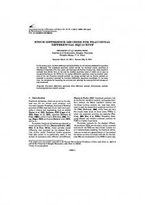
%%%Forward scheme for the heat equation: %%% INPUT %%%%%Advection velocity: mu = 1/16; %%%%Grid size; Use periodic boundary conditions X=1;M=10;Tend=4; h=1/(M+1); Dt=0.02; x= 0:h:X; %%% x(1) =0, x(2) = h, , ..., x(M) = X -h; x(M+1) = X; wn=sin(2*pi*x); time=0; mu = mu*Dt/h^2; while(time 0 and a < 0. Note that when a > 0 the characteristics are directed to the right and when a < 0 they are directed to the left. In some sense the sign of a indicates the direction of propagation of information. In fact the advection equation is also called the one-way wave equation, where a is the speed of propagation of the wave.
17
Time, t
t
+a
X= X0 +
at
X0 X=
X0
X0
a0
X
Figure 3: Characteristic lines for the advection equation. When a > 0 the characteristics are directed to the right and when a < 0 they are directed to the left. To find the solution u(x, t) at an arbitrary point (x, t) in the x-t plane, one needs to follow the characteristic line passing through (x, t) back to its original point at t = 0: (x0 , 0) with x = x0 + at. This leads to u(x, t) = u0 (x0 ) = u0 (x − at). (26) Example 2: Burger’s equation The Burger equation constitutes a somewhat more complex example a quasi-linear PDE. However, we still can, in principle, construct exact solutions using the method of characteristics. The system of characteristic equations for Burger’s equation is given by x˙ = z z˙ = 0. The characteristic solution is thus given by u(x(t), t) = u0 (x0 ); where x(t) = x0 + u0 (x0 )t.
(27)
Again note that the characteristics are straight lines and the solution is constant along the characteristic lines, with one important difference, however; the characteristic curves are no longer parallel to each other. As we will see below this has rather ”unpleasant” consequences. Provided the characteristics lines do not cross each other, which is guaranteed for at least a short period of time if the initial data u0 is continuous, the solution to Burgers equation is given by the following implicit formula u(x, t) = u0 (x − u0 (x0 )t), x = x0 + u0 (x0 )t. The characteristic lines associated with Burger’s equation are illustrated in Figure 4.
Exercise 3 Use the method of characteristics to solve the following quasi-linear equations. ut + xux = 0 18
t
Time, t
0)
+ X0
X 0(
u
X= X0
X= t
+a
X0
X0
u0’(x) > 0
u0’(X) < 0
X
Figure 4: Characteristic lines for Burger’s equation. When u′0 (x) > 0 the characteristics are divergent and when u′0 (x) < 0 they are converging toward each other. and ut + ux + x = 0. Write down the solution u(x, t) and draw the characteristic curves.
3.3
Notion of shocks and weak solutions
Note that because the slope of the characteristic curves x = x0 + u0 (x0 )t for Burger’s equation (4) increases when u0 (x0 ) increases and decreases when u0 (x0 ) decreases, the characteristic curves will accordingly diverge or converge toward each other (see Figure 4). Two convergent characteristic lines will ultimately cross each other at some point in the x-t plane. Beyond such intersection point the characteristic solution is no-longer valid, because the value of u(x, t) at such a point is not univalued–one can follow back either one of the two intersecting characteristic lines. One way to correct for this flaw is by stopping the characteristic lines as soon as they cross each other. Let Σ be the set of such crossing points in the x-t plane. The solution can then be defined on both sides of Σ by following the corresponding characteristic line back to its origin. Below we will see that Σ is a parametric curve on the form x = s(t) as show on Figure 5 and constitutes a curve of discontinuity for u(x, t). Such a curve is called a shock by analogy to gas dynamics. One of the main difficulties in practice is to find the shock curve x = s(t). For any given (x1 , t1 ) one has to determine whether two characteristic lines cross each other prior to time t1 along the curve x = x1 . Exercise 4 Show that a shock forms in the solution for Burger’s equation if and only if the initial condition satisfies u′0 (x) < 0 for some x 19
Σ Shock curve
Time, t
X
Figure 5: The shock curve Σ separates two regions of the x-t plane where the solution is smooth and is uniquely determined by the characteristics. The solution is discontinuous across the shock curve. and that the first time a shock occurs is given by T∗ = −
1 . minx u′0 (x)
After a shock is formed the solution u(x, t) is no longer valid in the classical sense except for its restrictions on the sub-domains located on either side on the shock. Nevertheless, such solution can be defined in the weak sense on the whole x-t plane. Definition 3 A function u(x, t) is said to be a weak solution for the conservation law ut + (f (x, t, u))x = 0 if for any test function φ(x, t) sufficiently smooth (e.g. C 1 ) with a compact support1 in (−∞, +∞)× (0, +∞), the solution u(x, t) satisfies Z +∞ Z +∞ Z +∞ Z +∞ u(x, t)φt (x, t) dxdt + f (x, t, u)φx (x, t) dxdt = 0. (28) 0
−∞
0
−∞
Remark: Note that according to the definition of weak solutions, given above, a C 1 function u(x, t) is a 1
i.e, there exist a bounded rectangle [t1 , t2 ] × [a, b] ⊂ (−∞, +∞) × (0, +∞) such that phi(x, t) = 0 out side this rectangle.
20
solution to the conservation law in the classical sense if and only if it is a solution in the weak sense. Therefore the notion of weak solutions is more general and the set of weak solutions contains discontinuous solutions as well as the classical C 1 solutions as a special subset. However, in some situations weak solutions are not unique, in the sense that one initial value problem can have more than one weak solution. Selecting the physically relevant solution can be tricky. For Burger’s equation for example, the physical solution coincides with the vanishing viscosity solution: u ¯(x, t) = lim uǫ (x, t) ǫ−→0
where
∂uǫ ∂ 2 uǫ ∂uǫ + uǫ =ǫ 2, ∂t ∂x ∂x under the grounds that the unviscid Burger equation is a mathematical idealization of the viscous Burger equation when the viscosity is very small. However, given two weak solutions it is not easy to identify which one is the limiting viscosity solution and which one is not. The answer is provided by an extra condition known as the entropy condition satisfied by the physical solution. We will see this in detail below. Note that the notion of weak solutions is very abstract and it is not obvious how one would handle this in practice. Nevertheless the theorem below provides the necessary ingredients both for constructing weak solutions and to gain physical insight.
Theorem 3 (Rankine-Hugoniot Condition) Let Σ be a curve in (−∞, +∞)×(0, +∞) parametrized by x = s(t). Let u(x, t) be a C 1 function on both side of but possibly not defined and discontinuous across the curve Σ. Assume u is a solution to the conservation law ut + (f (u))x = 0 on all points (x, t) not on Σ. For each point (x1 , t1 ) ∈ Σ we set u± (x1 , t1 ) =
lim
Ω1 ∪Ω2 ∋(x,t)−→(x1 ,t1 )±
u(x, t).
i.e. the limits from the right and from the left of Σ. Then u(x, t) is a weak solution for the conservation law if and only if the shock speed s˙ satisfies s˙ ≡
f (u+ ) − f (u− ) ds = . dt u+ − u−
(29)
The proof of this theorem is not terribly hard but it is quite technical and therefore left as an exercise for the interested student.
3.4
Discontinuous initial data and the Riemann problem
As it is pointed out above, the notion of weak solutions permits to define discontinuous solutions for conservation laws. Here we propose to construct such weak solutions with discontinuous initial 21
data. For simplicity, we consider the Burger equation with discontinuous initial data consisting of two constant states, a left and a right state: ut + uux = 0 � uL u0 (x) = uR
if x < 0 if x > 0.
(30)
The problem in (30) is known as the Riemann problem. We propose to construct simple weak solutions for the Riemann problem associated with Burger’s equation, using the Rankine-Huguniot condition (29). Shock waves: Consider a discontinuous function which consists of the two left and right constant states on both sides of a shock curve Σ : x = s(t); s(0) = 0 u(x, t) = uR if x > s(t)
(31)
u(x, t) = uL if x < s(t).
(32)
According to the Rankine-Hugoniot condition we have s˙ =
uR + uL 1 u2R − u2L = . 2 uR − uL 2
Note that the shock speed in this case is constant and the curve Σ is a straight line. Also recall that the speed of the characteristic lines on each side of the shock is simply uL and uR , respectively. Therefore the speed of the shock is exactly halfway between the left and right characteristic speeds. This has physical sense and the associated weak solution is called a shock wave. A rough sketch of the shock wave solution is given in Figure 6 for both cases when uR < uL and when uL > uR . Note that in the first case the characteristics run into the shock line and stop and therefore the solution on both sides of the shock is consistent with the characteristic solution while in the second case the characteristics diverge away and the region surrounding the shock is not reached by any of the characteristics. Rarefaction waves: Now assume that uL < uR so the characteristics emanating from both side of the discontinuity are divergent from each other. In this case we can actually construct another weak solution to the Riemann problem associated with the Burger’s equation. First note that for t > 0 the function u(x, t) = x/t, satisfies Burger’s equation ut + uux = 0. For t > 0 consider uL u(x, t) = x/t uR
if x < tuL if tuL < x < tuR if tuR < x.
(33)
First note that u(x, t) is a solution to Burger’s equation on each one of the designated parts of the domain and is continuous on the x-t plane. We can therefore show by simple integration by 22
time T Σ : x = (ur+ul)/2 t
111111111111111111111111 000000000000000000000000 000000000000000000000000 111111111111111111111111 000000000000000000000000 111111111111111111111111 000000000000000000000000 111111111111111111111111 000000000000000000000000 111111111111111111111111 000000000000000000000000 111111111111111111111111 000000000000000000000000 111111111111111111111111 000000000000000000000000 111111111111111111111111 000000000000000000000000 111111111111111111111111 000000000000000000000000 111111111111111111111111 000000000000000000000000 111111111111111111111111 000000000000000000000000 111111111111111111111111 000000000000000000000000 111111111111111111111111 000000000000000000000000 111111111111111111111111 000000000000000000000000 111111111111111111111111 000000000000000000000000 111111111111111111111111 000000000000000000000000 111111111111111111111111 000000000000000000000000 111111111111111111111111 000000000000000000000000 111111111111111111111111 000000000000000000000000 111111111111111111111111 000000000000000000000000 111111111111111111111111 000000000000000000000000 111111111111111111111111 000000000000000000000000 111111111111111111111111 000000000000000000000000 111111111111111111111111 000000000000000000000000 111111111111111111111111 000000000000000000000000 111111111111111111111111 000000000000000000000000 111111111111111111111111 000000000000000000000000 111111111111111111111111
u = ul
u = ur
X
time T
Σ : x = (ur+ul)/2 t 000000000000000000000000 111111111111111111111111 111111111111111111111111 000000000000000000000000 000000000000000000000000 111111111111111111111111 000000000000000000000000 111111111111111111111111 000000000000000000000000 111111111111111111111111 000000000000000000000000 111111111111111111111111 000000000000000000000000 111111111111111111111111 000000000000000000000000 111111111111111111111111 000000000000000000000000 111111111111111111111111 000000000000000000000000 111111111111111111111111 000000000000000000000000 111111111111111111111111 000000000000000000000000 111111111111111111111111 000000000000000000000000 111111111111111111111111 000000000000000000000000 111111111111111111111111 000000000000000000000000 111111111111111111111111 000000000000000000000000 111111111111111111111111 000000000000000000000000 111111111111111111111111 000000000000000000000000 111111111111111111111111 000000000000000000000000 111111111111111111111111 000000000000000000000000 111111111111111111111111 000000000000000000000000 111111111111111111111111 000000000000000000000000 111111111111111111111111 000000000000000000000000 111111111111111111111111 000000000000000000000000 111111111111111111111111 000000000000000000000000 111111111111111111111111 000000000000000000000000 111111111111111111111111 000000000000000000000000 111111111111111111111111
u = ul
u = ur
X Figure 6: Shock wave solutions for Burger’s equation. The two cases when uL > uR (top) and when uL < uR (bottom) are shown.
23
time T Rarefaction fan u = x/t 0000000000000000000000000 1111111111111111111111111 0000000000000000000000000 1111111111111111111111111 u = ul
1111111111111111111111111 0000000000000000000000000 0000000000000000000000000 1111111111111111111111111 0000000000000000000000000 1111111111111111111111111 0000000000000000000000000 1111111111111111111111111 0000000000000000000000000 1111111111111111111111111 0000000000000000000000000 1111111111111111111111111 0000000000000000000000000 1111111111111111111111111 0000000000000000000000000 1111111111111111111111111 0000000000000000000000000 1111111111111111111111111 0000000000000000000000000 1111111111111111111111111 0000000000000000000000000 1111111111111111111111111 0000000000000000000000000 1111111111111111111111111 0000000000000000000000000 1111111111111111111111111 0000000000000000000000000 1111111111111111111111111 0000000000000000000000000 1111111111111111111111111 0000000000000000000000000 1111111111111111111111111 0000000000000000000000000 1111111111111111111111111 0000000000000000000000000 1111111111111111111111111 0000000000000000000000000 1111111111111111111111111 0000000000000000000000000 1111111111111111111111111 0000000000000000000000000 1111111111111111111111111 0000000000000000000000000 1111111111111111111111111 0000000000000000000000000 1111111111111111111111111 0000000000000000000000000 1111111111111111111111111
u = ur
X Figure 7: Rarefaction wave solution for Burger’s equation. The rarefaction fan is shown. parts that indeed u(x, t) is a weak solution (see exercise 5 below). This type of solution is called a rarefaction wave by analogy to compressible gas dynamics and the solution u = x/t in the middle is referred to as a rarefaction fan, see the illustration in Figure 7. In summary, this shows that the Riemann problem for Burger’s equation has at least two weak solutions when uL < uR , one is a shock wave and the other is a rarefaction wave. Therefore, weak solutions for conservation laws are in general non-unique. Exercise 5 Let Ω be a bounded open set in the xt-plane. Let Σ be a curve passing through Ω dividing it onto two disjoint open subsets Ω1,2 such that Ω = Ω1 ∪ Σ ∪ Ω2 . Let φ(x, t) be a smooth function (e.g. C 1 ) supported in Ω, that is φ vanishes outside a compact set K ⊂ Ω. Let � u1 (x, t) if (x, t) ∈ Ω1 u(x, t) = u2 (x, t) if (x, t) ∈ Ω2 , where u1 , u2 are two C 1 functions satisfying the Burger equation in Ω1 , Ω2 , respectively. Use integration by parts to show that if in addition u is continuous across Σ, then Z 1 uφt + u2 φx dxdt = 0. 2 Ω Deduce that (33) is a weak solution to Burger’s equation.
3.5
Non-uniqueness of weak solutions and the entropy condition
As illustrated above with the example of a Riemann problem for Burger’s equation, weak solutions are non-unique. However, common sense suggests that for any given Cauchy problem, only one solution is physically relevant. We need an additional constraint to choose this physically relevant solution among all the weak solutions. In fact, in reality some viscosity is always associated with a given conservation law, so instead we have uǫt + (f (uǫ ))x = ǫ 24
∂ 2 uǫ , ∂x2
(34)
and the zero viscosity limit, ǫ −→ 0, is just a convenient mathematical idealization. It is true in many physical applications! Therefore, one universally accepted criterion states that the physically relevant weak solution for the conservation law ut + (f (u))x = 0 is the limit of the solution to the viscous equation (34) when ǫ −→ 0. On the other hand it is easy to show that, when combined with appropriate initial conditions, the latter has a unique solution. In practice, however, it is not clear how to establish if a given weak solution is actually the vanishing viscosity limit or not. The answer to this question is provided by the concept of entropic solutions. In a nutshell, the entropy condition states that the physical solution satisfies a general principle of thermodynamics that the entropy always decreases. It remains to find which among the weak solutions for a given conservation law satisfies the so-called entropy condition. There are many versions of the entropy condition for a given conservation law ut + (f (u))x = 0. i) A somewhat abstract version of the entropy condition, but with a clear physical significance is as follows. Given a conservation law ut + f (u)x = 0. A convex function Φ(u) and a flux function Ψ(u) are called an entropy/entropy flux pair if Ψ′ (u) = Φ′ (u)f ′ (u). Given an entropy/entropy flux pair (Φ, Ψ), a solution u for the conservation law is said to be an entropic solution if it satisfies ∂Φ(u) ∂Ψ(u) + ≤ 0, ∂t ∂x
(35)
in the weak sense. In many physical problem the entropy function Φ(u) is some measure of energy. It can be shown that for Burger’s equation, an entropy/entropy flux pair is given by 2 φ(u) = u2 ; Ψ(u) = u3 . 3 Here Φ(u) = u2 can be thought of as an energy density and Ψ(u) is the energy flux. The most apparent merit of this formulation is that it generalizes ’easily’ to systems of conservation laws. ii) A more practical version of the entropy condition is the following: � � 1 u(x + z, t) − u(x, t) ≤ C 1 + z, z, t > 0. t
(36)
iii) Perhaps the most abstract of them is due to Kruzkov. A (weak) solution to the conservation law is said an entropy solution in the sense of Kruzkov if, in addition, it satisfies Z ∞ Z +∞ sign(u − k) [(u − k)φt + (f (u) − f (k))φx ] dxdt ≥ 0 (37) 0
−∞
for all real constants k and all test functions φ ≥ 0. This version of the entropic solution is useful for theory. It is mainly used by mathematicians to prove existence and uniqueness theorems. 25
iv) Finally, we give the Lax entropy condition for shocks: A shock solution for the Riemann problem with left and right states uL , uR is said an entropic shock if the shock speed, s, ˙ satisfies f ′ (uR ) < s˙ < f ′ (uL ). (38) It is easy to see that only one of the two shock solutions for the Riemann problem for Burger’s equation is an entropic solution. Namely, the one associated with the case uR < uL (by the Lax entropy condition iv) as well as condition ii)). Moreover, it can be shown that the unique entropic solution in the case uL < uR is the rarefaction wave in (33).
4
Finite difference schemes for the advection equation
We start by discussing some basic simple finite difference schemes for the advection equation ut + aux = 0, where a is a positive constant. In principle these schemes are easily generalized to non-constant advection speeds with an arbitrary sign.
4.1
Some simple basic schemes
Throughout this paper we will assume the following discretization of space-time domain xj = j∆x; tn = n∆t, where ∆x, ∆t > 0 are respectively the spatial and time step sizes. We denote by unj the approximate/numerical solution to the solution u(xj , tn ). Perhaps the most obvious scheme to attempt for the advection equation, which unfortunately turns out to be unstable, is obtained by taking a first order forward finite differencing in time and a centred differencing in space: a∆t n (u − unj−1 ). (39) un+1 = unj − j 2∆x j+1 This scheme is referred to below, simply, as the centred scheme. Other simple possibilities are to take a first order derivative in space either to the left or to the right, combined with the forward differencing in time, yielding the so-called first order upwind and downwind schemes, respectively: un+1 = unj − j
a∆t n (u − unj−1 ) ∆x j
and
(40)
a∆t n (u − unj ). (41) ∆x j+1 Note that those two schemes are also known as the upstream and downstream schemes; depending on the application: hydrodynamics or gas dynamics (ocean v.s. atmosphere). The word upwind un+1 = unj − j
26
n+1
n+1 (a) n j−1
j
j+1
n+1
n+1
(b)
j−1
(d)
(c) n j
n j
j+1
j−1
j+1 n−1
Figure 8: Simple finite difference stencils for the advection equation: (a) forward in time centred in space, (b) upwind, (c) downwind, (d) leap-frog. refers to the fact that the finite differencing is performed in the direction opposite to the wind and downwind when the difference scheme follows the wind direction. Accordingly, when a < 0 the scheme in (41) becomes upwind and the scheme (40) becomes downwind.
Warning: As we will see below both the centred and the downwind schemes (39) and (41) are not recommended in practice because they are both unstable.
A slightly more sophisticated scheme is the leap frog scheme, which uses centred differences in both space and time: a∆t n (u − unj−1 ). (42) un+1 = ujn−1 − j ∆x j+1 The stencils for the four schemes listed above are given in Figure 8.
4.2
Accuracy and consistency
Definition 4 Let Lh (uh ) = 0 denote the numerical discretization using a certain method for a given partial differential equation denoted by L(u(x, t)) = 0, with a time step, ∆t, and grid spacing, ∆x. The numerical scheme is said to be consistent if the truncation error: τh = L(u) − Lh (u) satisfies lim
∆t,∆x−→0
τh = 0.
The scheme is said consistent of order (p, q) accurate or simply of order (p, q) if τh = O((∆x)p + (∆t)q ).
Examples: Consider the advection equation L(u) ≡ ut + aux = 0. 27
(43)
Using simple Taylor expansions, it is easy to see that the “centred scheme” (39) is consistent of order (2,1), namely ut + aux −
u(x, t + ∆t) − u(x, t) u(x + ∆x, t) − u(x − ∆x, t) ∆t (∆x)2 −a =− utt (x, η) − a uxxx (ξ, t) ∆t 2∆x 2 6 = O(∆t + (∆x)2 ).
i.e, this scheme is first order accurate in time and second order in space while the upwind and downwind schemes (40) and (41) are only first order in both space and time, τh (upwind/downwind) = O(∆t + ∆x). The leap-frog scheme (42), on the other hand is second order in both space and time τh (leapf rog) = O((∆t)2 + (∆x)2 ).
Exercise 6 Show that the leap-frog scheme (42) is second order accurate in both time and space.
4.3
Stability and convergence: the CFL condition and Lax-equivalence theorem
Definition 5 A numerical scheme for an evolution equation on a finite interval [0, T ], on the form un+1 = Sh (unj ) j is said stable if there exists a constant C > 0 such that ||un || ≤ C||u0 || for a certain norm ||.|| in RN , where N is the number of spatial grid points. Convergence of the numerical scheme The convergence of a numerical solution uh , obtained by a given numerical scheme, to the solution u of the original continuous equation is solved by the celebrated Lax-equivalence theorem.
Theorem 4 (Lax-equivalence theorem) The approximate numerical solution to a well posed linear problem converges to the solution of the continuous equation if and only if the numerical scheme is linear, consistent, and stable. The rate of convergence and the order of accuracy of the numerical solution is equal to the truncation error of the numerical scheme.
This elegant and powerful theorem is often summarized as follows consistency + stability = convergence .
28
von Neumann stability analysis The study of stability of a numerical scheme can be very tedious but the use of Fourier analysis when appropriate simplifies it a great deal. This idea was first used by von Neumann–apparently. For simplicity we assume that any discrete function, fj , i.e, defined on the grid points xj = j∆x by its values fj = f (xj ) can be expanded in discrete Fourier modes fj =
N/2 X
ρl eij∆x2πl + complex conjugate terms
l=0
√
where i = −1 and ρl are complex Fourier coefficients. N here is the number of spatial grid points and N/2 is known as the Nyquist number. It represents the largest wavenumber represented on an N-points grid. To simplify the notation we set φl = 2πl∆x. For the numerical solution unj evolving in the discrete time, tn , we have unj
=
N/2 X
ρnl eijφl .
l=0
Note that the upper script n is an index not a power. Theorem 5 (von Neumann Stability) A numerical scheme for an evolution PDE is stable (in the sense of von Neumann) if and only if the ratio ρl =
ρn+1 l ρnl
known as the amplification factor, of discrete Fourier coefficients of the numerical solution, satisfies
|ρl | ≤ (1 + ∆t), l = 0, · · · , N/2. Although the proof of this theorem is almost trivial, by Parseval’s equality, it has a huge significance and a big impact on our way of studying numerical methods, because it is very easy to use, especially for linear problems. In fact, when the numerical scheme is linear, it is enough to consider solutions on the form of a single Fourier mode unj = ρnl eijφl . (44) Plugging in (44) into the
• the centred scheme (39) yields
� � µ ρn+1 eijφl = ρn eijφl − ρn eijφl eiφl − e−iφl 2 29
where µ = a∆t/∆x. Thus the amplification factor, ρ ≡
ρn+1 ρn ,
is given by
ρ = 1 − µi sin(φl ). Thus, |ρ|2 = 1 + µ2 sin2 (φl ) > 1 + ∆t for some values of φl , for all ∆t sufficiently small, therefore the centred scheme (39) is unstable as suggested above. • the backward (in space) first-order scheme (40) yields ρ = 1 − µ(1 − e−iφl ) = 1 − µ(1 − cos(φl )) − iµ sin(φl ),
|ρ|2 = 1 + µ2 (1 + cos2 (φl ) − 2 cos(φl )) − 2µ(1 − cos(φl ) + µ2 sin2 (φl ) = 1 + 2µ2 + 2µ(1 − µ) cos(φl )) − 2µ.
Clearly if µ < 0, i.e a < 0, ρ > 1 + ∆t for some values of φl , for all ∆t sufficiently small, and when µ > 0 (a > 0), ρ ≤ 1 provided 0 ≤ µ ≤ 1. In other words, the upwind scheme is conditionally stable: ∆t ≤ ∆x/|a| or |a|∆t ≤ ∆x while the downwind scheme is always unstable. Similarly we can show that the forward-scheme (41) is stable if −1 ≤ µ ≤ 0 and unstable otherwise. Notice that the upwind scheme amounts to taking the derivative in the direction opposite to the advection speed, i.e, toward the direction where the information came from. • the leap-frog scheme (42) yields ρ2 = 1 − 2ρµi sin(φl ), which has 2 roots ρ± = −iµ sin(φl ) ±
q
1 − µ2 sin2 (φl ) if |µ| < 1
(45)
|ρ± |2 = 1 if |µ| < 1. When |µ| > 1, one can always find a value for φl for which the two roots ρ± are both imaginary and then necessarily one of them has to be strictly larger than one for all values of ∆t. Thus, as the upwind scheme, the leapfrog scheme is conditionally stable: ∆t ≤ ∆x/|a|. Note however, that unlike the previous schemes, von Neumann analysis for the leap-frog method leads to two amplitude modes, ρ± , for a given spatial mode exp(ijφl ). Nevertheless, as we will see below, only one of them is physical, namely, ρ+ , that is it represents an approximation (converges) to the exact solution, while the other one is an artifact of the numerical discretization. The latter is often called a computational or a parasitic mode.
CFL condition: The CFL condition, named after its discoverers, Courant, Friedrichs, and Lewy, states that if a difference scheme for an evolution equation is stable then the domain of dependence, corresponding to one time step, of the numerical scheme contains the domain of the dependence of the original continuous equation, when both the time step and the spatial grid size ∆t, ∆x −→ 0. Let’s first clarify the notion of domain of dependence. Given the partial differential equation, ut = F (u, ux )
30
Table 1: Some simple schemes for the advection equation and their properties. Scheme Order of accuracy Stability CFL condition Centred O(∆t + (∆x)2 ) Unstable Satisfied if ∆t ≤ ∆x/|a| Upwind O(∆t + ∆x) Stable if ∆t ≤ ∆x/|a| Satisfied if ∆t ≤ ∆x/|a| Downwind O(∆t + ∆x) Unstable Not satisfied Leap-frog O((∆t)2 + (∆x)2 ) Stable if ∆t ≤ ∆x/|a| Satisfied if ∆t ≤ ∆x/|a| with and initial condition u(x, t) = u0 (x), the domain of dependence of this equation at some point (x, t) is the set of all points x0 such that u(x, t) depends on the value of u0 at x0 ). For instance according to the solution by the method of characteristics to the advection equation (26), the domain of dependence of the advection equation is reduced to one point D(x,t) = {x0 = x − at} . The domain of dependence corresponding to one time step is D(x,t+∆t) = {(x − a∆t, t)} . This is illustrated in figure 9 for a > 0. The numerical domain of dependence of the numerical schemes considered so far are as follows Dcentred (x, t + ∆t) = {(x − ∆x, t), (x + ∆x, t)} Dbackward (x, t + ∆t) = {(x − ∆x, t), (x, t)} Df orward (x, t + ∆t) = {(x, t), ((x + ∆x, t)} Dleapf rog (x, t + ∆t) = {(x − ∆x, t), (x, t − ∆t), (x + ∆x, t)} Note that, as shown in Figure 9, the point (x−a∆x, t) is within the range the domain of dependence of all the above schemes so that the CFL condition is satisfied, provided the stability condition |∆t ≤ ∆x/|a| is satisfied, except for the forward scheme, corresponding to downwind differencing in this case, which explains its instability. Notice that this makes physical sense. As it is suggested by the method of characteristics, when a > 0 the solution to the advection equation uses information on the left to advance forward in time while the forward scheme uses information on the right. Note that the upwind and the leapfrog schemes do not have this problem. Also, the condition |a|∆t ≤ ∆x can be interpreted as a requirement that the numerical speed of propagation of information being smaller than the advection speed of the continuous problem. Interestingly note that the centred scheme (39) satisfies the CFL condition, if ∆t ≤ ∆x/|a|, as for the leap-frog scheme, but is not stable. This is a good example illustrating the important fact that the CFL condition is a necessary condition for stability but it is not sufficient. Table 1 summarizes the properties of the four simple schemes we have covered so far.
31
(X,t+Dt) t+Dt
t
X−aDt
X
X −Dx
X +Dx
Figure 9: Domain of dependence of the advection equation for a > 0 and the CFL condition.
4.4
More on the leap-frog scheme: the parasitic mode and the Robert-Asselin filter
According to table 1, the best we have, among the simple schemes seen so far, is the leap-frog scheme; it is stable and second order accurate in both space and time. Notice also as such it is relatively cheap and easy to implement. This may explain in part why this scheme is so popular in the engineering and atmosphere/ocean communities. However, it has at least two drawbacks: 1) it is a multistep (2 steps or 3 levels) scheme which means it needs the knowledge of the solution at two successive time steps in order to advance to the next one and 2) it carries a parasitic mode which may ruin the numerical solution when used for long time integrations, if it is not filtered carefully. More details on the leap-frog scheme and its parasitic mode can be found in the literature (e.g. Durran). Here we briefly illustrate and demonstrate the behaviour of this parasitic mode and give a strategy for controlling it in practice. Recall the von Neumann amplification factors associated with the leap-frog scheme p ρ± = −iσ ± 1 − σ 2 where we set σ = µ sin(φl ). Since |ρ± | = 1 we have iψ±
ρ± = e
, ψ± = arctan
�
−σ √ ± 1 − σ2
with ψ0 = arcsin(σ) we have ψ+ = −ψ0 , ψ− = −π + ψ0 ,
ρ+ = e−iψ0 , ρ− = ei(−π+ψ0 ) ,
32
�
and the Fourier mode solution for the leap-frog scheme is given by unj = (c1 ρn+ + c2 ρn− )ejiφl = c1 ei(jφl −nψ0 ) + c2 (−1)n ei(jφl +nψ0 ) ≈ c1 e2πli(xj −atn ) + c2 (−1)n e2πli(xj +atn )
(46)
where we used the fact that µ = a∆t/∆x, φl = 2πl∆x, n∆t = tn ; j∆x = xj and the approximation arcsin(σ) ≈ σ; sin(φl )/φl ≈ 1. The expression in (46) clarifies that the term representing ρ+ has the form f (x − at) and therefore provides an approximation for the solution to the advection equation while the remaining term represents a wave moving in the opposite direction (to the left) and its amplitude oscillates between positive and negative values. Clearly, the latter is an artifact of the numerical discretization, called the computational or parasitic mode, and may lead to serious damage to the solution if it is not controlled in some way. There are many ways how to control the computational mode. One of them is to make sure that the ’extra initial condition’, i.e, solution at first time step, needed to advance the leap-frog method is chosen so that the coefficient c2 , of the parasitic mode, is zero fin the decomposition of u0 into Fourier modes. One easy way to guarantee that initially the parasitic mode is zero is to set as second initial data at t = ∆t, required to evolve the multi-step leap-frog method, to be X 0 ijφl u1j = ρ+ l ρl e l
given at t = 0 we have u0j =
X
ρ0l eijφl .
l
However, we known that for long integration periods the parasitic mode can be excited and grow just from round-off errors. A safe commonly used strategy for controlling the computational mode for the leap-frog scheme, known as the Robert-Asselin filter, is given next. The Robert-Asselin filter consists in averaging the solution at every time step by using the previous and the future solution, at t − ∆t and t + ∆t, respectively, by introducing an extra-filtering step. Let u ¯nj denote the solution filtered in such a way. The two step leap-frog plus Robert-Asselin filtering scheme is given by un+1 =u ¯jn−1 − µ(unj+1 − unj−1 ) j
− 2unj + u ¯jn−1 ), u ¯nj = unj + γ(un+1 j
(47)
where γ is a small filtering parameter usually taking to be γ = 0.06. Some atmospheric models used for cloud physics use values as large as γ = 0.3 (Durran). It is important to note that the filtering step destroys the second order accuracy in time and the resulting scheme is only first order.
4.5
The Lax-Friedrichs scheme
The Lax-Friedrichs scheme is a clever modification for the unstable centred scheme (39), which makes it stable. It consists of replacing the term unj by the average from the neighbouring cells to 33
obtain
unj+1 + unj−1 � a∆t n − uj+1 − unj−1 . (48) 2 2∆x This is the celebrated Lax-Friedrichs scheme. As the centred scheme the Lax-Friedrichs scheme (48) is second order accurate in space and first order in time. However, it is stable under the CFL condition |µ| ≡ |a|∆t/∆x < 1 . In fact, the associated von Neumann amplification factor is given by ρ = cos(φl ) − iµ sin(φl ) un+1 = j
=⇒ |ρ|2 = cos(φl )2 + µ2 sin(φl )2 ≤ 1 if |µ| ≤ 1.
Exercise 7 Show that the Lax-Friedrich’s scheme is first order in time and second order in space and that its amplification factor is given by ρ = cos(φl ) − iµ sin(φl ). The apparent advantages of the Lax-Friedrichs scheme, when compared to the three other stable schemes listed above is that it is second order in space and is a one step method, therefore easier to implement in practice compared to the leap-frog method. However, it is only first order accurate in time, which limits its use in practical applications and it is extremely dissipative as we will see below.
4.6
Second order schemes: the Lax-Wendroff scheme
Perhaps the simplest way to achieve a one-step (2 levels) scheme, which is second order in both time and space for the advection equation, is to resort to Taylor expansion in the time variable u(x, t + ∆t) = u(x, t) + ∆tut (x, t) +
(∆t)2 utt (x, t) + · · · 2
using the advection equation ut = −aux yields u(x, t + ∆t) = u(x, t) − a∆tux (x, t) +
a2 (∆t)2 uxx (x, t) + · · · 2
Now, we use second order centred differencing to approximate the spatial derivatives ux and uxx to obtain the Lax-Wendroff scheme = unj − un+1 j
� µ2 n � µ n uj+1 − unj−1 + uj+1 − 2unj + unj−1 . 2 2
(49)
It is easy to show that the Lax-Wendroff scheme (49) is second order accurate in both space and time and it is stable under the CFL condition a∆t/∆x ≤ 1. The amplification factor for this scheme is ρ = 1 − iµ sin(φl ) − µ2 (1 − cos(φl )).
34
Exercise 8 Show that the Lax-Wendroff scheme is second order in both time and space and it is stable under the CFL condition a∆t/∆x ≤ 1. If instead we use a second order approximation of the first order space derivative in the Taylor expansion using points that are only in the upwind direction, namely, xj−2 , xj−1 , xj when a > 0, we obtain the following scheme, known as the Beam-Warming’s scheme: un+1 = unj − j
� µ2 n � µ 3unj − 4unj−1 + unj−2 + uj − 2unj−1 + unj−2 . 2 2
(50)
This scheme can be derived by using polynomial interpolation. In fact, let P2 (x) = uj−2 +
uj − 2uj−1 + uj−2 uj−1 − uj−2 (x − xj−2 ) + (x − xj−1 )(x − xj−2 ) ∆x 2(∆x)2
be the 2nd degree polynomial interpolating u on the grid points xj , xj−1 , xj−2 . Using this polynomial to approximate the derivatives ux , uxx at x = xj yields the Beam-Warming scheme. The details are left as an exercise for the student. Note that because the stencil of the Beam-Warming scheme uses two grid cells on the left of xj , the associated CFL condition becomes 0 ≤ a∆t/∆x < 2. In fact we can show that this scheme is stable under this CFL condition. Compared to Lax-Wendroff’s scheme this new scheme allows larger time steps. However, if the advection speed is not too large the time step might be restricted to that of the Lax-Wendroff for accuracy reasons.
Exercise 9 Show that the Beam-Warming scheme is second order in both time and space and it is stable under the CFL condition a∆t/∆x ≤ 2. Exercise 10 Derive the version of the Beam-Warming scheme when a < 0.
4.7
Some numerical experiments
Here we assess the performance of each one of the (stable) methods listed above, for the advection equation, the interval [0, 1] with periodic boundary conditions and two different initial data. We consider a smooth initial condition consistent of a hump-like shaped profile, u0 (x) = exp(−100(x − .5)2 ), and a non-smooth–piece-wise constant, initial condition, called here a square wave u0 (x) = 0 if |x − 0.5| > 0.25, u0 (x) = 1 if |x − 0.5| < 0.25. The advection velocity is assumed constant and normalized to a = 1 and integrate to time t = 1 so that the initial profile is moved forward by a distance equal to the length of the interval [0, 1] and by periodicity we have u(x, t = 1) = u0 (x). We use a mesh size ∆x = 0.01 and a time step ∆t = 0.008 corresponding to a Courant number µ = ∆t/(|a|∆x) = 0.8. 35
1
1 Exact upwind Lax−Friedrichs
0.8
Exact Leap frog 0.8
0.6
0.6
0.4
0.4
0.2
0.2
0 −0.2
0
0.2
0.4
0.6
0.8
1
1.2
1.2
0 −0.2
0.2
0.4
0.6
0.8
1
1.2
0.6
0.8
1
1.2
1.2 Exact Lax−Wondroff
1
0.8
0.6
0.6
0.4
0.4
0.2
0.2
0
0
0
0.2
Exact Beam−Warming
1
0.8
−0.2 −0.2
0
0.4
0.6
0.8
1
1.2
−0.2 −0.2
0
0.2
0.4
Figure 10: Solution to the advection equation using different finite difference schemes. Case of a smooth hump advected periodically through the interval [0, 1]
36
1.5
Exact upwind Lax−Friedrichs
1
1
0.5
0.5
0
0
−0.5 −0.5
1.5
0
0.5
1
Exact Lax−Wondroff
−0.5 −0.5
1
0.5
0.5
0
0
0
0
0.5
1
0.5
1
1.5 Exact Beam−Warming
1
−0.5 −0.5
Exact Leap frog R−A Leap frog
1.5
0.5
1
−0.5 −0.5
0
Figure 11: Same as Fig. 10, except for the non-smooth, piece-wise constant, square wave. Note that for this case results with both the plain leap-frog and leap-frog combined with the Robert-Asselin filter are shown.
37
In Figure 10, we plot the numerical solutions, obtained with each one of the 5 methods, against the exact solution for the advection equation. In Figure 11 we report the similar plots corresponding to the non-smooth square wave. Here we note a few important points. • First, for the smooth solution in Figure 10, as expected the second order methods (leapfrog, Lax-Wendroff, and Beam-Warming) are highly accurate whereas the first order upwind and Lax-Friedrichs methods yield very unsatisfactory results. They both suffer from an excessive dissipation; that is the wave amplitude decays in time. Surprisingly, the upwind scheme seem to perform better than Lax-Friedrichs, although, the latter is second order accurate in space. • Second, for the non-smooth case in Figure 11, on the other hand, the two first-order methods seem to perform better than the three second order methods, although they tend to smooth out the discontinuity. The second order schemes exhibit high oscillations near the discontinuities. This is typical for high order methods, they are exhibit an oscillatory behaviour near shocks. Note also that Lax-Wendroff is somewhat better than Beam-Warming and that LaxWendroff produces oscillations behind the shock while the oscillations in the Beam-Warming are located in front of the discontinuity. Below, we will see how to design high resolution or non-oscillatory scheme which in principle are second order accurate in regions where the solution is smooth and only first order–non oscillatory near the shocks. • Third, note that the leap-frog scheme seem to the exhibit the worst oscillatory behaviour for the non-smooth solution. In fact, most of this is due to the presence of the computational mode which tend to amplify the oscillations. Things look a lot better when the the computational mode is controlled by the Robert-Asselin filter. Notice that the filtered leap-frog is somewhat between the Lax-Wendroff and a first order method for it exhibits some oscillations behind the shock and smooths out the discontinuity at the same time. The matlab programs used to generate those results can be obtained upon request from the author. Below, we analyze the different schemes in detail to understand better their performances.
4.8
Numerical diffusion, dispersion, and the modified equation
Consider the upwind scheme (40) for the advection equation. With some simple manipulations this scheme can be rewritten as n+1
∆t uj 1 − ujn−1 ) + (un+1 j 2∆t 2 or
un+1 − ujn−1 j 2∆t
+a
− 2unj + ujn−1 (∆t)2
unj+1 − unj−1 2∆x
unj+1 − unj−1 a∆x unj+1 − 2unj + unj−1 + = −a 2∆x 2 (∆x)2
n+1 n−1 n n n n a∆x uj+1 − 2uj + uj−1 ∆t uj − 2uj + uj = + . 2 (∆x)2 2 (∆t)2
(51)
For all practical purposes this scheme can be thought of as an approximation for the diffusive advection equation a∆x ∆t ut + aux = uxx + utt , 2 2 38
with a second order truncation error, O((∆x)2 + (∆x)2 ). Differentiating the advection equation once with respect to t, yields utt = auxt = (aut )x = a2 uxx , i.e, the diffusive equation above becomes � � a∆x a∆t ut + aux = 1− uxx . 2 ∆x This equation is sometimes called the modified equation approximated by the upwind scheme to the second order. In essence, the upwind scheme approximates the viscosity solution introduced in (34) corresponding to the advection equation with the viscosity ǫ = a∆x 2 (1 − µ) where µ = a∆t/∆x is the Courant number. On the one hand this can make us believe that in fact the upwind scheme computes the right physical solution, by approximating the vanishing viscosity solution, and on the other hand it provides an explanation on the poor performance of this scheme, especially in the case of the smooth solution in Figure 10, of under-predicting the solution. Note the viscosity coefficient, introduced by the upwind scheme, is zero if the Courant number if choosing to be perfectly one. Such choice is avoided in practice because it may lead to numerical instabilities because of round-off errors. Further as noted above a little viscosity is necessary to guarantee convergence to the physical solution. This phenomenon is known as numerical dissipation or diffusion. It is due to the term n+1
∆t uj 2
n n n a∆x uj+1 −2uj +uj−1 + 2 2 (∆x)
n−1 −2un j +uj (∆t)2
on the right hand side of (51). In fact, multiplying the viscous advection equation by u and integrate on [0, 1] yields Z 1 Z Z d 1 u2 a 1 2 dx + uuxx dx. (52) (u )x dx = ǫ dt 0 2 2 0 0 Where we used uut = (u2 )t /2 and uux = (u2 )x /2 . By integration by parts we have Z 1 Z 1 Z 1 2 1 (ux )2 dx (ux ) dx = − uuxx dx = uux |0 − 0
0
0
provided the boundary terms vanish, which happens if we use periodic or homogeneous Dirichlet or Neumann boundary conditions. The second term on the right of the integral equation (52) vanishes for the same reason and yields the following energy dissipation principle Z 1 Z d 1 u2 (ux )2 dx < 0 if ux 6= 0. dx = −ǫ dt 0 2 0 Thus if integrated to infinity the upwind scheme will smooth out all the gradients in the solution and will ultimately converge to a constant-flat solution. As we can surmise from Figures 10 and 11, the Lax-Friedrichs scheme is more dissipative than the upwind scheme. Indeed, the Lax-Friedrichs scheme is equivalent to − unj un+1 j ∆t
n+1 n−1 n n n n unj+1 − unj−1 (∆x)2 uj+1 − 2uj + uj−1 ∆t uj − 2uj + uj +a = − . 2∆x 2∆t (∆x)2 2 (∆t)2
(53)
which yields a dissipative modified equation, which is the second order approximation of the Lax2 2 ∆t 2 2 Friedrichs scheme, with a viscosity ǫ = (∆x) 2∆t − a 2 = (∆x) (1 − µ )/(2∆t) which is typically larger than that of the upwind scheme. 39
This dissipation or diffusivity problem is typical to first order schemes for hyperbolic systems. Let us now consider the second order schemes and derive the modified equations associated with those schemes. Since they are already second order accurate, we should consider approximations with an order of accuracy higher than two. Below, we take a slightly different route than it is done above, to derive the modified equation. Namely, we use Taylor expansion as to compute the truncation error but instead we keep the first neglected term and add it to the advection equation to form the modified equation. For the leap-frog method we have un+1 − ujn−1 j 2∆x
+a
unj+1 − unj−1 (∆t)2 (∆x)2 = ut + uttt (x, t)+O((∆t)4 )+aux +a uxxx (x, t)+O((∆x)4 ) 2∆x 6 6
(because all even terms in the Taylor series cancel out). Again using the advection equation we have: uttt = −a3 uxxx and therefore the modified equation, which is approximated to the fourth order by the leap-frog scheme, is ut + aux = −
� a(∆x)2 1 − µ2 uxxx . 6
(54)
This equation is known as the dispersive wave equation. First, it is easy to show that this equation conserves energy (see exercise 11 below). This is consistent with the fact that the von Neumann amplification factors for the leap-frog method satisfy |ρ± | = 1 when µ < 1. Second, dispersion refers to a physical system where waves of different wavelengths propagate at different wave speeds. Let’s look at wave like solution on the form u = ei(kx−ωt) for the dispersive wave equation. Here k = 2πl is the wavenumber, ω is called the phase or frequency, ω/k defines the phase speed, the speed at which the wave propagates. Plugging this ansatz into (54) yields, the dispersion relation ω = ak −
� a(∆x)2 1 − µ2 k 3 , 6
� 2 i.e the phase speed, ck = a − a(∆x) 1 − µ2 k2 , depends highly on the wavenumber, and higher the 6 wavenumber faster the wave disturbance moves relative to the advective motion. Short waves move relatively faster. This is very unlike the plain-original advection equation were all waves move at the same speed–the advection speed a. Now, we reconsider the von Neumann amplification factors for the leap-frog method in (45). Recall that we have two solutions (one is physical and the other is a numerical artifact), which we denote here by: u+ = ei(kj∆x−nψ0) ; u− = (−1)n ei(kj∆x+nψ0 ). Let us consider only the physical mode, u+ . From the discussion above, using n = tn /∆t, the associated phase speed is given by c+ =
arcsin(µ sin(φl )) ψ0 = k∆t k∆t 40
Using Taylor expansion to expand both the sine and the arcsine functions, for small φl values (resolved modes), yields ψ0 ≈ µφl −
(∆x)2 µ (1 − µ2 )φ3l = a∆tk − a∆t(1 − µ2 )k3 6 6
which implies that the phase speed of the physical mode for the leapfrog scheme satisfies c+ ≈ a − a
(∆x)2 (1 − µ2 )k2 . 6
This matches exactly the expression for ck found above, using the dispersive wave equation. Now, we can explain why in Figure 11, the leapfrog scheme exhibits oscillations. They result from the fact that the small truncation errors located near the discontinuity, which also accumulate with time, are viewed as wave disturbances of much shorter wavelengths which then propagate at their own speeds different from that of the actual solution. Recall that the amplification factors for the previous two first order schemes, namely the upwind and the Lax-Friedrichs, are respectively given by ρuw = 1 − µ(1 − cos(φl )) − iµ sin(φl ) and ρLF = cos(φl ) − iµ sin(φl ). In the light of the analysis done in the previous paragraphs for the leap-frog scheme, we set ρn ≡ e−in∆tω where ω is a generalized phase so that ℜ(ω)/k yields the phase speed of the numerical wave solution and ℑ(ω) yields the exponential growth or damping rate of the wave amplitude. We have for the upwind and Lax-Friedrichs schemes, respectively, e−iωuw ∆t = 1 − µ(1 − cos(φl )) − iµ sin(φl ) , e−iωLF ∆t = cos(φl ) − iµ sin(φl ). For small ω∆t, we have e−iω∆t ≈ 1 − iω∆t. Hence ωuw ∆t ≈ µ sin(φl ) − iµ(1 − cos(φl )) and ωLF ∆t ≈ µ sin(φl ) − i(1 − cos(φl )). First note that both schemes have quite strong damping rates, ℑ(ωuw ) =
1 1 − cos(φl ) a µ (1 − cos(k∆x)) ≈ − k2 ∆x, ℑ(ωLF ) = − ≈ − ∆xk2 , ∆t 2 ∆t 2µ
respectively, and consistently with the previous results, the LF scheme being more damped–by a factor of 1/µ. With φl = k∆x, the phase speeds are equal and are given by � � ℜ(ωLF ) a k2 (∆x)2 ℜ(ωup ) = = sin(k∆x) ≈ a 1 − . k k k∆x 6 This clearly shows that both schemes are dispersive, similarly to the leap-frog scheme. Nevertheless, small wave disturbances typically occurring at the grid scale decrease in magnitude at a faster rate than the domain-scale physical wave. 41
Now we turn to the Lax-Wendroff and Beam-Warming schemes. We have ρLW = 1 − iµ sin(φl ) − µ2 (1 − cos(φl )) yielding
µ2 µ sin(φl ) − i (1 − cos(φl )), (55) ∆t ∆t i.e, for the phase speed, we have the same dispersive behaviour as for the previous schemes but a much smaller damping rate ωLW =
ℑ(wLW ) = −
µ2 2 µ2 (1 − cos(φl )) ≈ − k (∆x)2 , ∆t 2∆t
of the same order as the phase speed deviation. For grid scale disturbances, the wavenumber, k, µ2 scales as 1/∆x, therefore the damping rates for those small scale waves is on the order O( 2∆t ) which seems to be small, explaining the propagation of the small oscillations, in Figure 10, away from the discontinuity before they get damped. More importantly note the propagation of the oscillations for the Lax-Wendroff scheme, in Figure 10, to the left of the discontinuities, is associated with the fact that according to the dispersion relation (55) smaller wavelength disturbances move slower than those with larger wavelengths. We have a similar behaviour for the Lax-Wendroff scheme. But the Beam-Warming scheme exhibits somehow larger amplitude oscillations moving to the right, which seems to anticipate that the Beam-Warming scheme has both a weaker damping rate and dispersive phase speeds characterized by smaller wavelengths propagating faster than larger ones. The details are left as an exercise.
Exercise 11 Show that the dispersive wave equation ut + aux = γuxxx conserves energy, that is d dt
Z
0
1
u2 dx = 0. 2
Exercise 12 Determine the exponential damping rate and the phase speed for the Beam-Warming scheme. Deduce that this scheme is dispersive and that wave disturbances with larger wavenumbers (smaller wavelengths) propagate faster than those with smaller wavenumbers.
42
1
0.9
Initial Exact upwind Lax−Friedrichs
0.8
0.7
0.6
0.5
0.4
0.3
0.2
0.1
0 −0.2
0
0.2
0.4
0.6
0.8
1
1.2
Figure 12: Riemann Problem for Burger’s equation solved with both upwind and Lax-Friedrichs schemes, showing that the upwind schemes predicts a wrong shock speed.
5 5.1
Finite volume methods for scalar conservation laws Wrong shock speed and importance of conservative form
Consider Burger’s equation with the discontinuous initial condition 1 ut + (u2 )x = 0 2 � 1 if x < 0.25 u0 (x) = 0 if x > 0.25.
(56)
We view Burger’s equation as an advection equation with a non-linear advection speed a(u) = u and attempt to solve this problem with both the upwind and Lax-Friedrichs methods. The upwind scheme is generalized to Burger’s equation as follows. un+1 = unj − j
� ∆t max(unj , 0)(unj − unj−1 ) + min(unj , 0)(unj+1 − unj ) . ∆x
(57)
Whereas the formula for Lax-Friedrichs’ scheme amounts to approximating the flux derivative using centred differences. � ∆t 1 (unj+1 )2 /2 − (unj−1 )2 /2 . un+1 = (unj+1 + unj−1 ) − j 2 2∆x
(58)
The results are shown in Figure 12 where the two numerical solutions are compared to the exact solution to the Riemann problem. Note that the Lax-Friedrichs method predicts well the propagation of the shock wave, with a significant smearing of the discontinuity, as excepted, due its high viscosity, while the upwind scheme predicts a steady solution which doesn’t change with time. In fact, this latter result can be easily recovered analytically from the upwind scheme. The numerical solution in this case remains zero on the right of the shock because the advection velocity is zero and remains one on the left because the backward finite difference derivative is zero.
43
The main reason for why the Lax-Friedrichs scheme out performs the upwind scheme, in this case, is because the former has a conservative form. A numerical scheme for a conservation law ut + (f (u))x = 0 is said conservative if it can be written on the form � � un+1 = unj + Fj+1/2 − Fj−1/2 . j
(59)
Where Fj+1/2 , called a numerical flux which is in some sense an approximation of the flux f (u) at the cell interface, xj+1/2 = xj + ∆x/2. Here we show that indeed the Lax-Friedrichs scheme has a conservative form. Let µ 1 LF Fj+1/2 = (unj+1 − unj ) − (f (unj+1 ) + f (unj ). 2 2 Then the Lax-Friedrichs schemes can be written as LF LF = unj + Fj+1/2 un+1 − Fj−1/2 . j
Thus it is conservative. We will see below that, the Lax-Wendroff and the Beam-Warming methods are also conservative. Remark: It is worthwhile noting that the formula for the Lax-Friedrichs flux, F LF , at the interface j + 1/2, is the average of the left and right fluxes, f (uj ), f (uj+1 ), plus a centered difference, uj+1 − uj , suggesting a diffusive term. Thus, the Lax-Friedrichs scheme can be viewed as a discrete version of the diffusive equation ut + (f (u) − ǫux )x = 0 where ǫ =
(∆x)2 2∆t
is the viscosity coefficient.
Convergence of Conservative Schemes: It is shown in the literature that if a numerical scheme for a conservation law ut +(f (u))x = 0 is consistent, stable, and has a conservative form, then the resulting numerical solution converges to a weak solution to the conservation law. This statement can be viewed as an extension of the Lax-equivalence theorem to non-linear conservation laws. Notice however, since weak solutions are not unique, it is not guaranteed that the numerical solution obtained by a consistent, stable, and conservative scheme converges to the physical entropic solution. For that some extra-properties of the numerical scheme are needed to enforce the entropy condition.
5.2
Godonuv’s first order scheme
Let xj = j∆x, j = · · · , −2, −1, 0, 1, 2, · · · and tn = n∆t, n = 0, 1, 2, · · · be a discretization of the space-time domain (x, t). We divide the real line into sub-intervals [xj−1/2 , xj+1/2 ], called grid cell, where xj+1/2 = xj + ∆x/2. We define the cell average of the solution u(x, t) at each grid cell as Z xj+1/2 1 n u(x, tn )dx. (60) u ¯j = ∆x xj−1/2 44
Consider the conservation law ut + (f (u))x = 0. Next, we integrate this equation on the rectangle [tn + tn+1 ] × [xj−1/2 , xj+1/2 ], often called the control or finite volume, hence the name finite volume method. We have Z tn+1 Z xj+1/2 Z tn+1 Z xj+1/2 (f (u(x, t)))x dxdt = 0 ut (x, t)dxdt + xj−1/2
tn
or Z xj+1/2 xj−1/2
u(x, tn+1 )dx−
Z
xj−1/2
tn
xj+1/2
u(x, tn )dx+
tn+1
Z
tn
xj−1/2
(f (u(xj+1/2 , t)))dt −
Z
tn+1
tn
(f (u(xj−1/2 , t)))dt = 0.
Dividing by the mesh size ∆x and introducing the averages u ¯nj above, yields
u ¯n+1 =u ¯nj − j where n Fj+1/2 =
1 ∆t
Z
i ∆t h n n , Fj+1/2 − Fj−1 ∆x
(61)
tn+1 tn
(f (u(xj+1/2 , t)))dt,
is the average flux of u through the interface x = xj+1/2 , tn ≤ t ≤ tn+1 . Provided we find an adequate numerical approximation to the time integral, the formula (61) provides a numerical scheme for the conservation law, in conservative form. Piecewise constant approximations and the Riemann problem at the cell interfaces: Assume that at time t = tn , the cell averages u ¯nj are known. Consider the approximation: u(x, tn ) ≈ u ¯nj , if xj−1/2 ≤ x ≤ xj+1/2 . Then finding an approximation for the flux Fj+1/2 , amounts to solving the Riemann problem ut + (f (u))x = 0, t ∈ [tn , tn+1 ] � uL if x < xj+1/2 u(x, tn ) = uR if x > xj+1/2
(62)
where the left and right states are given, respectively, by uL = u ¯j and uR = u ¯nj+1 . To compute the flux Fj+1/2 we need to know the solution u along the interface x = xj+1/2 , tn ≤ t ≤ tn + ∆t. We introduce the shock speed at the cell interface, s˙ =
f (uR ) − f (uL ) , uR − uL
according to the Rankine-Hugoniot jump condition. Under the condition that f (u) is convex, using the method of characteristics, introduced above, we have, for tn ≤ t ≤ tn + ∆t, uL if f ′ (uL ) > 0 & f ′ (uR ) > 0 uR if f ′ (uL ) < 0 & f ′ (uR ) < 0 u(xj+1/2 , t) = uL if f ′ (uL ) ≥ 0 & f ′ (uR ) ≤ 0 & s˙ > 0 (63) ′ ′ uR if f (uL ) ≥ 0 & f (uR ) ≤ 0 & s˙ < 0 u∗ if f ′ (uL ) ≤ 0 & f ′ (uR ) ≥ 0, 45
where in (63), u∗ , called a sonic point, is defined such that f ′ (u∗ ) = 0 and corresponds to a rarefaction wave solution. Notice that the convexity of f guarantees that u∗ exists and is unique. Note also the fist four cases correspond either to an entropic shock solution where, according to Lax’s criterion, f ′ (uL ) ≥ s˙ ≥ f ′ (uR ) so that uj+1/2 = uL if s˙ > 0 and uj+1/2 = uR if s˙ < 0 or a rarefaction waves where the rarefaction fan is either completely to the left or completely to right of the interface according to whether f ′ (uR,L ) < 0 or f ′ (uR,L ) > 0, respectively. The last case, however, corresponds to rarefaction wave where the rarefaction fan contains characteristics going both to the left and to the right. It is called a transonic rarefaction, by analogy to gas dynamics, where such a rarefaction happens when the fluid on one side of the wave moves at a speed smaller than the speed of sound (subsonic) and on the other side it moves with a speed larger than the speed of sound (supersonic). Here we show that the sonic point u∗ is in fact the root of the equation f ′ (u∗ ) = 0. Assume f ′ (uL ) < 0 < f ′ (uR ), then in this case there is a rarefaction wave connecting the left and right states. Inspired by the solution to Burger’s equation, a rarefaction wave solution is sought on the form u(x, t) = v(x/t). Plugging this ansatz into the conservation law ut + (f (u))x = 0, yields −
1 x ′ v (x/t) + f ′ (v(x/t))v ′ (x/t) = 0. t2 t
Hence
x . t Along the interface x = 0 we have u∗ = u(0, t) = v(0) and f ′ (v(0)) = 0. f ′ (v(x/t)) =
The celebrated Godunov’s method is now obtained by simply using the solution to the Riemann problem in (63) at each interface xj+1/2 to computes the numerical fluxes Fj−1/2 , Fj+1/2 in (61), yielding
Fj+1/2
f (uL ) f (uR ) f (uL ) = f (uR ) f (u∗ )
if f ′ (uL ) > 0 & f ′ (uR ) > 0 if f ′ (uL ) < 0 & f ′ (uR ) < 0 if f ′ (uL ) ≥ 0 & f ′ (uR ) ≤ 0 & s˙ > 0 if f ′ (uL ) ≥ 0 & f ′ (uR ) ≤ 0 & s˙ < 0 if f ′ (uL ) ≤ 0 & f ′ (uR ) ≥ 0.
(64)
Notice that the solution u∗ in (62) can be replaced by the shock solution, i.e, uR if s˙ < 0 and uL if s˙ > 0, even when f ′ (uL ) < 0 < f ′ (uR ), and will still provide a weak solution satisfying the Rankine-Hugoniot jump condition, but as we already know this will lead to an unphysical weak solution which violates the entropy condition. The resulting numerical solution is referred to as an all shock solution and provides an approximation to the weak solution to the conservation law, which is not necessarily the physically relevant–entropic solution. Case of the advection equation and Stability of Godunov’s method If we replace the conservation law by the simple advection equation with a positive advection speed, a > 0, then the solution to the Riemann problem at the cell interface, xj+1/2 , reduces to u(xj+1/2 , t) = uj , 46
1
0.9
Initial Exact Godunov Lax−Friedrichs
0.8
0.7
0.6
0.5
0.4
0.3
0.2
0.1
0 −0.2
0
0.2
0.4
0.6
0.8
1
1.2
Figure 13: Same as Figure 12 but with Godunov’s method instead of the upwind scheme. and Godunov’s method reduces to the upwind scheme u ¯n+1 =u ¯nj − j
a∆t n (¯ u −u ¯nj−1 ). ∆x j
(65)
Recall that the upwind method is stable under the CFL condition. Therefore, provided the CFL condition max(f ′ (uL ), f ′ (uR ))∆t ≤ ∆x (66) is satisfied, Godunov’s method is stable. Consistency and convergence Moreover, given the way the fluxes were computed, i.e, using the exact solution of the Riemann problem using first order approximation of the initial data, namely piecewise constant cell averages, we can show that Godunov’s method is consistent of order 1 in both space and time, just like the upwind scheme. Moreover, since it is also conservative by construction, Godunov’s method is guaranteed to convergence to the entropic weak solution, provided we always choose the entropic solution for the Riemann problem. The numerical test of Figure 12, is repeated with the Godunov method and the results are shown in Figure 13, where Godunov’s method is compared to the Lax-Friedrichs method. As we expect Godunov’s method predicts the right shock speed and has much less dissipation than the Lax-Friedrichs method. However, one big disadvantage of Godunov’s method is that it requires the solution of a Riemann problem at each cell interface and every time step. This can be very costly especially for non-linear systems of conservation laws. An other serious shortcoming of Godunov’s method is that it is only first order in both time and space. This limits its use in practice but it constitutes an important cornerstone for more sophisticated so called high resolution methods developed below.
5.3
High resolution, TVD, and MUSCL schemes
As noted above one of the major shortcomings of Godunov’s method is that it is only first accurate in both space and time. As noted above a crucial step in deriving this method is the piecewise 47
constant approximation step, when the solution u(x, t) at time t = tn is approximated by the cell average u(x, tn ) ≈ u ¯nj , xj−1/2 ≤ x ≤ xj+1/2 ,
to advance to the next time step, tn+1 , which is only a first order approximate/interpolation. Since Godunov’s method computes the cell averages at each new time step, this piecewise approximation appears to be very convenient, indeed. Given the cell averages u ¯nj , we can use piecewise linear interpolation to yield a second order reconstruction u(x, tn ) ≈ u ˜(x, tn ) ≡ u ¯nj + σj (x − xj ), xj−1/2 < x < xj+1/2 , which can be used instead to advance the solution to next step (see Figure 14). The slopes σj can be computed in many different ways; using many different finite differencing formulas as we will see below. To illustrate let us consider the advection equation ut + aux = 0, a > 0. Given the piecewise linear reconstruction values, u ˜(x, tn ), at time t = tn , the ”exact” solution for this equation at t = tn + ∆t is given by u(x, tn + ∆t) = u ˜(x − a∆t, tn ). Provided a∆t/∆x < 1, we have � n u ¯j−1 + σj−1 (x − a∆t − xj−1 ) u(x, tn + ∆t) = u ¯nj + σj (x − a∆t − xj )
if xj−1/2 < x < xj−1/2 + a∆t if xj−1/2 + a∆t < x < xj+1/2 .
(67)
˜ Averaging u ˜(x, tn+1 ) on the intervals (xj−1/2 , xj+1/2 ), Z σj−1 xj−1/2 +a∆t a∆t n u ¯ + (x − a∆t − xj−1 )dx+ u ¯n+1 = j ∆x j−1 ∆x xj−1/2 Z xj+1/2 σj ∆x − a∆t n u ¯j + (x − a∆t − xj )dx, ∆x ∆x xj−1/2 +a∆t yields the cell averages at tn + ∆t, given by u ¯n+1 =u ¯nj − j
a∆t a∆t n (¯ u −u ¯nj−1 ) − (∆x − a∆t) (σj − σj−1 ). ∆x j 2∆x
(68)
If we set the slopes to zeros, σj = 0, then we recover the first order Godunov (upwind) method in (65). A second order scheme is obtained, if the slope is choosing to be a first order finite differencing formula which approximates the derivatives ux (xj , tn ) in the j’th grid cell, using neighbouring cell average values. The following three choices of slopes yield three popular second order schemes Centered: Upwind: Downwind:
u ¯j+1 − u ¯j−1 (Fromm) 2∆x u ¯j − u ¯j−1 σj = (Beam-Warming) ∆x u ¯j+1 − u ¯j σj = (Lax-Wendroff). ∆x
σj =
48
Exercise 13 Show that when a < 0 the second order scheme for the advection equation using piecewise linear reconstruction is given by u ¯n+1 =u ¯nj − j
a∆t a∆t n (¯ u −u ¯nj ) + (∆x + a∆t) (σj+1 − σj ). ∆x j+1 2∆x
(69)
Reconstruct, Solve, Average: The algorithm followed above to derive Godunov’s method as well as its second order version for the advection equation involves three main steps. 1) Reconstruct: Given the cell averages u ¯nj , we (re)construct piecewise constant or piecewise linear approximations u ˜(x, tn ) ≈ u ¯jn or u ˜(x, tn ) ≈ u ¯jn + σj (x − xj ), xj−1 < x < xj+1/2 2) Solve: Solve the Riemann problem ut + (f (u))x = 0, tn ≤ t ≤ tn+1 , u(x, tn ) = u ˜(x, tn ) 3) Average: Average the solution at tn+1 Z xj+1/2 1 n+1 u ¯j = u(x, tn+1 ) dx. ∆x xj−1/2 A few remarks on the Reconstruct-Solve-Average algorithm: Note the first step is crucial, it sets the order of accuracy of the method. Piecewise constants yield a first order method while a piecewise linear approximation yields a second order scheme. In fact methods using parabolic approximations exist are often used in practice, they are known are PPM (for piecewise parabolic methods). Piecewise parabolic reconstruction yields a third order method and so on. For, the second step it is desirable to be able to solve the conservation law exactly. This is possible in the case of the advection equation and for the conservation law in general when piecewise constants are used in step one, yielding Godunov’s method. But in general, we need to resort to quadrature formulas to approximate the flux integrals along the time interval [tn , tn + ∆t]. Finally, when a finite volume method, such as Godunov’s, is applied to a conservation law, it yields the average values u ¯n+1 directly, which takes care of step three. j High order finite volume method for conservation laws Recall the finite volume derived in (61) for Godunov’s method =u ¯nj − u ¯n+1 j where n Fj+1/2
1 = ∆t
Z
i ∆t h n n , Fj+1/2 − Fj−1 ∆x tn+1
tn
(f (u(xj+1/2 , t)))dt.
49
To reconcile with the case when u(x, t) is not piece-wise constant at time t = tn , we approximate the time integral by a rectangular rule yielding an Euler step � ∆t � ˜ n n (70) Fj+1/2 − F˜j−1/2 u ¯j+1 = u ¯nj − ∆x where n F˜j+1/2 = f (u∗ (xj+1/2 , t+ n )). Here u∗ (xj+1/2 , t+ n ) = lim u(xj+1/2 , t) t−→tn
is obtained by solving the Riemann problem with left and right states uL = u ˜(xj+1/2,− , tn ), uR = u ˜(xj+1/2,+ , tn ) where again u ˜(xj+1/2,− , tn ) =
u ˜(x, tn ) and u ˜(xj+1/2,+ , tn ) =
lim
x−→xj+1/2,xx
j+1/2
Note that in the case of a piecewise constant approximation these limits are simply uL = u ¯nj and n+1 uR = u ¯j , and the solution to the Riemann problem is constant on the time interval [tn , tn + ∆t], provided the CFL condition ∆t max(|f ′ (uR )|, |f ′ (uL )|) ≤ ∆x is satisfied. Note this is not true for higher order reconstructions. To obtain higher order accuracy in time, we often use a predictor-corrector scheme such as the mid-point Runge-Kutta method in place of the first-order Euler step (70):
� ∆t � ˜ n n Fj+1/2 − F˜j−1/2 2∆x ∆t � ˜ n+1/2 ˜ n+1/2 � n =u ¯j − Fj+1/2 − Fj−1/2 ∆x
u ¯j+1/2 = u ¯nj − u ¯j+1 where
(71)
n+1/2 F˜j+1/2 = f (u∗ (xj+1/2 , t+ n+1/2 )).
Oscillations and TVD methods Recall from Figure 11 that one major problem with second order methods is that they tend to generate unphysical oscillations near discontinuities. One way to control these oscillation is to use a hybrid method where the second order reconstruction is limited to regions where the solution, u, is smooth and use a first order method in regions where u presents discontinuities of some sort. To find an intelligent way to do so, we first introduce a mathematical tool to control those oscillations. This is achieved by the total variation, which is introduced next. Definition 6 The total variation (TV) of a real valued function f is given by TV(f ) = sup
+∞ X
j=−∞
|f (ξj+1 ) − f (ξj )|
where the supremum is taken on all subdivisions · · · < ξ−1 < ξ0 < ξ1 < · · · of the real line. 50
To help develop some intuition, we list a few properties of TV. • If f (x) is monotonic (i.e, non-increasing or non-decreasing) on some interval [a, b], then the total variation of f on [a, b] is given by TV[a,b] (f ) = |f (b) − f (a)| • If f (x) is piecewise constant on the line segments (xj−1/2 , xj+1/2 ), then TV(f ) =
+∞ X
j=−∞
|f (xj+1 ) − f (xj )|,
i.e, the sum of all the jumps of f . • If f (x) is piecewise linear on the line segments (xj−1/2 , xj+1/2 ), then TV(f ) =
+∞ X
j=−∞
+ |f (x− j+1/2 ) − f (xj−1/2 )| +
+∞ X
j=−∞
− |f (x+ j+1/2 ) − f (xj+1/2 )|,
i.e, the sum of the variations within each one of the line segments plus all the jumps across the interfaces. • If f is differentiable, then TV(f ) =
Z
+∞ −∞
|f ′ (x)|dx.
Since the exact solution to the advection equation simply propagates at a constant speed, its TV doesn’t change with time. Moreover, it can be shown that the total variation for an entropic solution for a conservation law, in general, doesn’t increase with time. It can decrease after a shock but never increases. However, this is not always the case for the numerical solution. Clearly the oscillations generated by the second order schemes in Figure 11 do increase the TV of the numerical solution. A reasonable way to attempt to avoid those unphysical oscillations, is thus to require that the total variation of the numerical solution does not increase.
Definition 7 The numerical scheme u ¯j+1 = u ¯nj −
� ∆t � ˜ n n Fj+1/2 − F˜j−1/2 ∆x
is said to be total variation diminishing (TVD) if
TV(¯ un+1 ) ≤ TV(¯ un ).
(72)
For instance we can show that the average step in the Reconstruct-Solve-Average algorithm does actually diminish total variation. Therefore, when the slopes are set to zeros, σj = 0, the upwind scheme for the advection equation is TVD. 51
Definition 8 A numerical scheme un+1 = H(unj−k , unj−k+1 , · · · , unj+l ) j is said to be monotone if
∂H ≥ 0, η = j − k, · · · , j + l. ∂uη
One important property of monotone schemes is that they do not create new local maxima or minima: max un+1 ≤ max unj , and min un+1 ≥ min unj j j
As such monotonic schemes are TVD. On the other hand TVD schemes are monotonicity preserving. A numerical scheme is said to be monotonicity preserving if monotonic data remains monotonic: n+1 ≤ un+1 · · · unj−1 ≤ unj ≤ unj+1 ≤ · · · =⇒ · · · un+1 j+1 ≤ · · · j−1 ≤ uj
We have the following general statement monotonic schemes ⊂ TVD schemes ⊂ monotonicity preserving schemes. It is easy to show that, under the CFL condition, a∆t ≤ ∆x, Godunov’s method for the advection equation is monotonic. In fact, for a > 0, we have un+1 = H(unj , unj−1 ) ≡ (1 − µ)unj + µunj−1 . j Therefore it is TVD as noted above. Unfortunately, it is not possible to construct linear second order schemes which are monotonic, according to the following theorem due to Godunov. In agreement with the fact that second order schemes exhibit oscillations. Theorem 6 (Godunov) A linear monotonic scheme is at most first order accurate. In order to achieve high order schemes without unphysical oscillatory behaviour we need to make schemes which are intrinsically nonlinear. A family of such schemes are the hybrid schemes mentioned above, which are second order in smooth regions and only first order near shocks, to avoid oscillations. To guarantee that our hybrid numerical scheme remains TVD and second order accurate in smooth regions, we must choose the slopes σj so that the TV of the reconstructed function is not larger than that of the discrete cell averages u ¯nj . This is achieved by defining the slope σj as a non-linear n function of the data u ¯j in such a way to control the total variation. The associated non-linear function is called a limiter and methods based on this idea are known as slope-limiter methods, first introduced by van Leer when he derived his famous MUSCL schemes (Monotonic UpstreamCentered Schemes). Perhaps the simplest choice of a limiter, which guarantees second order accuracy in regions where u is smooth and satisfies the TVD property at the same time, is the minmod limiter: σj = minmod(
¯nj − u ¯nj−1 u¯nj+1 − u ¯nj u , ) ∆x ∆x 52
(73)
where
a minmod(a, b) = b 0
if |a| < |b| and ab > 0 if |b| < |a| and ab > 0 if ab ≤ 0.
Note that when a, b have the same sign, the minmod function chooses the one which is smaller in magnitude and when ab ≤ 0, it returns zero. Instead of using the downwind slope, yielding the Lax-Wendroff scheme, or the upwind slope, leading to the Beam-Warming scheme, the minmod limiter chooses the one which is smaller in magnitude. When the upwind and downwind slopes have opposite sign, the reconstructed cell value is kept constant. This latter must correspond to a local minimum or a local maximum, and the minmod limiter tends to preserve the local extrema, hence avoiding to create overshootings and undershootings near those extrema. Thus it does not increase TV and does not generate oscillations. A more popular choice of limiter, due to van Leer, is the MC-limiter (monotonized-centered limiter): ¯nj u¯nj − u ¯nj−1 u¯nj+1 − u ¯nj−1 u¯nj+1 − u ,2 ,2 ) σj = minmod( 2∆x ∆x ∆x Note, the MC-limiter chooses the smallest in magnitude between the centred-differences, corresponding to Fromm’s method, and twice the upwind or the downwind formulas, and returns zeros when there is a change is sign. This limiter yields highly accurate centered slopes in smooth regions and sharper resolution near discontinuities. Flux-limiters Using piecewise linear reconstruction for the advection equation yields (see (68) and (69)) u ¯n+1 =u ¯nj − j where n Fj+1/2
=
∆t n n (F − Fj−1/2 ) ∆x j+1/2
a a¯ unj + (∆x − a∆t)σj 2
a a¯ unj+1 − (∆x + a∆t)σj+1 2
if a > 0 if a < 0.
Introducing the negative and positive parts of a
a+ = max(a, 0), a− = min(a, 0) the flux Fj+1/2 can be rewritten in a compact form as Fj+1/2
� � 1 δt|a| =a u ¯j+1 + a u ¯j + |a| 1 − δj , 2 ∆x +
−
(74)
where δj is the jump in u ¯ across the upwind interface; δj = u ¯j − u ¯j−1 if a > 0 and δj = u ¯j+1 − u ¯j if a < 0. We introduce the upwind side of j as J=
�
j−1 j+1 53
if a > 0 if a < 0
Piecewise linear Piecewise constant
j−1
j
j+1
Figure 14: Piecewise constant (dashed) and piecewise linear reconstructions. and the jump ∆¯ uj = u ¯j+1 − u ¯j . We define
θ=
∆¯ uJ . ∆¯ uj
and let δj = φ(θ)∆¯ uj in (74), where φ is a non-linear function of θ, called a flux-limiter, which is defined so that the resulting scheme is second order accurate in smooth regions and TVD at the same time. Some linear choices of φ yield the popular second order (linear) schemes:
φ(θ) = 0 :
upwind
φ(θ) = 1 :
Lax-Wendroff
φ(θ) = θ : 1 φ(θ) = (1 + θ) : 2
Beam-Warming Fromm,
which are of course not TVD according to Godunov’s theorem. While some clever non-linear choices yield high resolution–TVD methods. The following are the most popular ones: φ(θ) = max(0, min(1, θ)) :
minmod
φ(θ) = max(0, min((1 + θ)/2, 2, 2θ)) :
MC-limiter
φ(θ) = max(0, min(1, 2θ), min(2, θ)) : 1+θ : φ(θ) = 1 + |θ|
superbee
54
van Leer.
They all have their strengths and weaknesses, depending on the application. Those are well documented in the literature (see LeVeque’s book: finite volume methods for hyperbolic problems, for examples). The performance of each of the choices of limiters listed above is shown on the different panels in Figure 15, for both the smooth and the non-smooth/square wave. We see that in general the TVD limiters capture very well both the smooth solution (with an accuracy comparable to the second order schemes) and the non-smooth square wave. The second order methods have an oscillatory behaviour near the discontinuity and the upwind method is too diffusive.
References [1] Crispin W. Gardiner, 2004, Handbook of Stochastic Methods: for Physics, Chemistry and the Natural Sciences, Springer. [2] Randall J. LeVeque, 2002, Finite Volume Methods for Hyperbolic Problems (Cambridge Texts in Applied Mathematics),Cambridge University Press. [3] Dale Durran, 1998, Numerical Methods for Wave Equations in Geophysical Fluid Dynamics, Springer.
55
2 1.5
2 Exact minmod
1.5
1
1
0.5
0.5
0 −0.5
0
0.5
0 −0.5
1
2 1.5
Exact superpee
2 1
0.5
0
0 −0.5
0
0.5
1
0
0.5
1
0
0.5
1
0
0.5
1
3 Exact 2 Lax−Wendroff
Exact upwind
1
1
0.5
0
0
0.5
−1 −0.5
1
3
3
Exact 2 Beam−Warming
2
1
1
0
0
−1 −0.5
0.5
Exact van Leer
−1 −0.5
1
2
0 −0.5
0
3
1
1.5
Exact MC
0
0.5
−1 −0.5
1
Exact Fromm
Figure 15: Performance of the different limiter functions listed in the text for both the smooth and non-smooth data.
56