Comparison of finite element and finite difference

Comparison of finite element and finite difference modelling results with measured performance of a reinforced soil wall Damians I.P.1, Bathurst R.J.2, Josa A.1 and Lloret A.1 1 School of Civil Engineering, Universitat Politècnica de Catalunya - BarcelonaTech, Barcelona, Spain 2 Royal Military College of Canada, Kingston, Ontario, Canada ABSTRACT The performance of a metallic reinforced soil segmental retaining wall is examined in a systematic manner using two numerical modelling approaches. Finite element modelling was carried out using the commercial program PLAXIS and finite difference modelling using the commercial program FLAC. Numerical model results using both approaches were compared against measurements recorded for a well-instrumented full-scale 3.6-m high wall constructed with a sand backfill, modular-block facing, and steel reinforcement (welded wire mesh). This paper presents measured and predicted toe loads, facing displacements, and reinforcement connection loads at end of construction and during subsequent staged surcharge loading approaching failure. Both numerical models have been verified against recorded measurements. The sensitivity of the assigned backfill soil friction angle on the magnitude and distribution of reinforcement connection loads is also examined. The paper concludes with a summary of lessons learned to achieve satisfactory agreement between predicted performance and wall measurements using both modelling approaches. RÉSUMÉ La performance d’un mur de soutènement en sol renforcé par bandes métalliques est examinée de manière systématique en utilisant deux approches de modélisation numérique. La modélisation par éléments finis a été réalisée en utilisant le programme commercial (PLAXIS) et la modélisation par différences finies en utilisant le programme commercial (FLAC). Les résultats des modèles numériques, utilisant les deux approches, ont été comparées avec les mesures enregistrées pour un mur d’échelle réelle de hauteur de 3,6 m bien instrumenté construit avec un remblai de sable, une paroi de blocs modulaires et une armature en acier (treillis soudé). Cet article présente les charges mesurées et prévues au pied de la fondation, les déplacements de la paroi et les charges de connexion du renforcement à la fin de la construction et durant l’application par paliers des surcharges subséquentes approchant la rupture. Les deux modèles numériques ont été vérifiés par rapport aux mesures enregistrées. La sensibilité des propriétés du sol de remblai sur la magnitude et la distribution des charges de renforcement est également examinée. L’article se termine par un résumé des leçons apprises pour parvenir à un accord satisfaisant entre la performance prévue et les mesures prises sur le mur en utilisant les deux approches de modélisation.

1

INTRODUCTION

Mechanically stabilized earth (MSE) walls (reinforced soil walls) are complex mechanical systems. They are comprised of a hard concrete facing in most cases, granular soil backfill and polymeric or steel reinforcement layers. Many walls today are constructed with a drystacked modular concrete block facing. Current design methods give recommendations for the internal stability design of these systems so that reinforcement layers do not fail or deform excessively within the soil backfill or at the connections (FHWA 2009). These design methods are based on closed-form solutions adapted from conventional earth pressure theory. For geosynthetic (polymeric) reinforced soil walls there is evidence that these design methods are very conservative (Bathurst et al. 2008). For metallic reinforced soil systems the conservatism is not as great because load equations have been empirically adjusted using measured loads from instrumented walls (Allen et al. 2004). Regardless of the reinforcement type, current design methods are most applicable for walls with simple configurations and competent foundation conditions. For walls falling outside

of design guideline envelopes, numerical modelling may be the only alternative for design. However, there are a number of questions that must be addressed when using numerical models for design: 1. Has the numerical model been verified against one or more instrumented structures (Carter et al. 2000)? 2. Are project-specific material properties available? 3. Will different numerical modelling packages give different design outcomes and, if so, are the differences important? The current investigation is focused on the last question. Two widely used numerical modelling software packages that use different numerical solution schemes are used to predict performance features of a wire mesh (metallic) reinforced soil wall. One software package is the program FLAC which uses the finite difference method (FDM) solution scheme and the other is the PLAXIS software package that uses the finite element method (FEM). The 2D simulation results are compared to measurements taken from the well-instrumented full-scale experiment noted above and previously reported in the literature.

A very brief description of both software programs follows in the following sections. 2

EXPLICIT FINITE DIFFERENCE METHOD: FLAC

FLAC (Fast Lagrangian Analysis of Continua) is a commercial software program developed by ITASCA Consulting Group for engineering mechanics computations. Since 1986 several updated versions have appeared, and the program currently offers a wide range of capabilities to solve complex problems in soil and rock mechanics (Itasca 2005). FLAC is based on the finite difference method (FDM) to solve partial differential equations. In the FDM the system equations are directly replaced by an algebraic expression at discrete points. The main characteristic of this procedure is that it is able to use an explicit resolution algorithm. Since no global stiffness matrix is formed, large calculations can be made without excessive memory requirement. Due to the explicit solution method, FLAC allows numerical paths to be followed up to plastic collapse. This allows the user to simulate unstable physical processes without numerical divergence issues. The program is well-suited to model large-strain scenarios. For domain discretization, FLAC divides the continua into a finite difference mesh (numerical grid) composed of quadrilateral elements, each of which is internally subdivided into two sets of superimposed constant strain triangles. Examples of numerical simulation of geosynthetic reinforced soil walls using the program FLAC have been reported by Hatami and Bathurst (2005, 2006) and Huang et al. (2009). Bathurst et al. (2012) used the program FLAC to investigate the influence of foundation compressibility on the behaviour of nominal identical walls constructed with geosynthetic and steel soil reinforcement. 3

FINITE ELEMENT METHOD: PLAXIS

PLAXIS development began in 1987 at Delft University of Technology with the initial objective to develop a userfriendly finite element code for the analysis of river embankments on soft soils found in Holland. The code has been greatly extended since that time and the PLAXIS software can be used for many geotechnical engineering problems (PLAXIS 2008). In the finite element method (FEM) the domain is divided into elements. Nodes (where the displacements are calculated) and Gauss points, where loads are calculated, are defined within each element. In PLAXIS 2D, the surfaces and areas are formed by 6-node or 15node triangles and the element stiffness matrixes are evaluated by 3-point and 12-point Gaussian integrations for 6-node and 15-node triangles, respectively. Due to the general nonlinear relationship between stress increments and strain increments, an approximate formulation of the global stiffness matrix must be formed beforehand, and a global iteration process with a certain tolerance is required to satisfy both the equilibrium

condition and constitutive relation under the given boundary and initial conditions. Damians et al. (2013a, b) used PLAXIS to investigate the influence of concrete facing unit bearing pad number and compressibility on the behaviour of steel strip reinforced soil walls. 4

GENERAL APPROACH

This paper describes the results of a series of numerical simulations with both software programs (FLAC and PLAXIS) that were carried out on a full-scale plane strain 3.6-m high (H) modular block wall constructed with welded wire mesh reinforcement and sand backfill soil. The accuracy of the FLAC model to predict performance features of the physical wall has been demonstrated in previously published work (Hatami and Bathurst 2005 and 2006, and Huang et al. 2009). In the current study the same verified numerical code is used to model the same wall and to compare predictions with a similar numerical model using the PLAXIS software. The paper presents measured and predicted toe loads, facing displacements, and reinforcement loads at end of construction and during subsequent staged surcharge loading. A single example of a parametric sensitivity analysis illustrating the influence of friction angle on connection loads is given at the end of the paper. 5

NUMERICAL MODELS

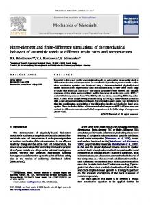
5.1 General FLAC (version 5.0) and PLAXIS (version 9.2) programs were used to carry out the numerical simulations. As mentioned earlier, the reference case was an instrumented 3.6-m high modular block wall with welded wire mesh reinforcement and sand backfill soil. The physical model was seated on a rigid concrete foundation. The same geometry and boundary conditions were assumed for both numerical models matching the physical experiment (Figure 1). The foundation is assumed as rigid, and the toe of the facing was restrained horizontally by a stiff element with an axial spring stiffness of 4 MN/m/m matching the value deduced from measurements at this boundary in the physical test. The FLAC model domain was discretized using a 50×50 numerical grid (Figure 1a). A total of 2009 6-node triangular elements were generated for the PLAXIS model (Figure 1b). As noted earlier, PLAXIS allows the use of 15-node elements. However, solving the model constructed with 15-node elements greatly increased computation time with no detectable difference in numerical results. In order to make fair comparisons between the PLAXIS model and the large strain (Lagrangian) FLAC model, the mesh updating option was selected at each construction step during the PLAXIS simulation.

where Jt(ε,t) is the equivalent tangent stiffness function; J0(t) is the initial tangent stiffness; η(t) is a scaling function; Tf(t) is a stress-rupture function for the reinforcement; ε is strain and t is time (i.e., duration of loading equal to the time to construct the wall). PLAXIS uses tension elements (called “geogrids”) to model soil reinforcement layers. These line elements are assigned an axial stiffness (J = EA) and a maximum tension force (Np). PLAXIS does not provide for userdefined constitutive models for the geogrid elements, so it is was not possible to implement the hyperbolic model described above for the general case of polymeric materials that have stiffness that is strain- and timedependent. However, the reinforcement material used in the instrumented wall case was a metallic welded wire mesh (WWM). Therefore the PLAXIS linear-elastic stiffness model was used for this relatively inextensible reinforcement. In the FLAC model, setting η(t) = 0 in Equation 1 results in the same linear-elastic stiffness for the metallic WWM as in the PLAXIS simulation. Reinforcement model parameters are summarized in Table 1.

a) FLAC model numerical grid

5.2.2 Backfill soil

b) PLAXIS model mesh

Linear elastic model with Mohr-Coulomb failure criterion was used as the constitutive model for the backfill material in both numerical models. This material is high quality medium sand with a narrow size distribution. The model parameters were taken from independent laboratory tests reported by Hatami and Bathurst (2005) and are summarized in Table 2. Hatami and Bathurst (2006) and Huang et al. (2009) showed that the linear elastic-plastic model gave sensibly the same results as more complex soil models with hyperbolical stress-strain behaviour at least for working stress conditions.

Figure 1. Numerical models

5.2.3 Interfaces

8ᵒ

The same material properties and construction steps matching the physical experiment were used for both models. Construction involved backfilling in 150-mm-thick layers and then applying a transient uniform pressure of 16 kPa to simulate compaction equipment effects. Following construction, a uniform distributed surcharge load (q) was applied in 10 kPa pressure increments up to 80 kPa. 5.2 Material properties 5.2.1 Reinforcement The following hyperbolic model proposed by Hatami and Bathurst (2006) was used in the FLAC model:

Jt (ε,t) =

1  1 η(t)  J0 (t)  + ε J (t) T f (t)   0

[1]

In the FLAC model case, linear spring-sliders with interface shear strength defined by the Mohr-Coulomb failure criterion were used for the facing-backfill and reinforcement-backfill interfaces (Itasca 2005). In the PLAXIS model, interfaces were modeled with zerothickness elements (PLAXIS 2008). Typically, PLAXIS interfaces are defined by a reduction factor that is related to the maximum strength of the soil at the interface (i.e., rigidly bonded interface case). This assumption is reasonable for ultimate failure since this interface can be controlled by the friction angle of the soil, but it is only a simplifying assumption for the estimation of the interface stiffness. An alternative strategy is to model the interfaces in PLAXIS by assigning a different constitutive behaviour to interface elements (i.e., different from the surrounding soil). The results of independent block-block direct shear tests (Hatami and Bathurst 2005) were used to determine the model parameters for block-block interfaces and the same parameters were used in both models (Table 3). It should be noted that for the PLAXIS case, the shear modulus value (G) was obtained directly from the

Table 1. Welded wire mesh reinforcement properties Model

Parameters

Values

FLAC

J0(t) (kN/m), η(t), Tf(t) (kN/m)

3100, 0, 7

PLAXIS

EA (kN/m), Np (kN/m)

3100, 7

Table 2. Sand backfill properties Model parameter

Value 3

 (unit weight, kN/m )

16.8

E (elastic modulus, MPa)

80

 (Poisson’s ratio)

0.3

 (friction angle, degrees)

44

ψ (dilatancy angle, degrees)

11

c (cohesion, kPa)

0.2

6

Value: Block-block

Soil-block

FLAC model:  (friction angle, degrees)

57

44

ψ (dilation angle, degrees)

0

11

c (cohesion, kPa)

46

0

Kn (normal stiffness, MN/m/m)

1000

100

Ks (shear stiffness, MN/m/m)

40

1

1

2

57

44

ψ (dilation angle, degrees)

0

11

46

G (shear modulus, MPa)

1.5

0 1

30 and 3

The calculations were made using a computer with an ‘Intel Core 2 Duo Pa8600’ (2.40 GHz) central processor unit. The times to solve the entire problem (i.e., construction and surcharging) were about 20 minutes using FLAC and 30 minutes using PLAXIS. All measured values shown in the figures to follow correspond to the average measured values at each location (no range bars are shown) in order to simplify data presentation. 6.2 Toe reactions

PLAXIS model:  (friction angle, degrees) c (cohesion, kPa)

RESULTS

6.1 General

Table 3. Interface properties Parameter

factor with respect to the backfill strength (i.e., 1.0, 0.8, 0.6 and 0.4). Nevertheless, no significant variations were detected in numerical results. Hence, a perfectly bonded interface was used in the final simulation runs (reduction factor equal to 1). The reinforcing materials were assumed to be perfectly bonded to the backfill sand (i.e., rigid interface). This assumption was judged to be reasonable based on the good agreement between numerical predictions that used the same model and measurements of reinforcement loads and strains in two physical tests used to validate the numerical model (Hatami and Bathurst 2006; Huang et al. 2009).

2

Equivalent to Ks-value in FLAC model according to the relation: G = Ks × (virtual thickness / contact area between blocks). Used at the back of the facing blocks and for the horizontal heel of the blocks at the back of the facing column.

interface shear stiffness used in the FLAC model (Ks). This was possible due to the known values of the blockto-block contact geometry and the virtual thickness of the interface FEM model (which depends on the mesh element size and which was 10.5 mm in this case). Soil-block interface parameter values are summarized in Table 3. The FLAC model was simplified by assuming a flat rough facing surface in contact with the backfill (hence, the interface failure criterion is the same as the soil). The interface shear stiffness (Ks) was assumed to be very low. In PLAXIS, the back of the facing column surface was assumed to be stepped as in the physical case. This left a very low density volume of soil below the heel of each block that was assigned very low shear stiffness and no tensile strength. The back vertical sides of the blocks were assumed to have a different reduction

Figure 2a shows the horizontal and vertical components of the total toe load which were generated during construction of the wall. Predicted values for both models are very similar and both sets of predictions are judged to be in good agreement with measured results. Shown in the same plot is the self-weight of the facing column which plots as a straight line. The total predicted and measured vertical loads are greater than the facing column self-weight due to down-drag forces that are generated at the back of the wall facing due to hanging-up of the soil at the connections and interface friction between the concrete facing blocks and the sand backfill. The down-drag loads are generated due to relative vertical movement of the backfill soil during compaction and subsequent outward facing column movement during surcharging. Figure 2b shows the horizontal and vertical toe load components during surcharging. The PLAXIS model can be seen to generally underestimate the measured load values. The FLAC model can be seen to over-estimate measured values at the highest surcharge pressures. 6.3 Vertical foundation pressures Figures 3a and 3b show the normalized vertical pressure distribution over the rigid concrete foundation upon which the wall was constructed (σv/[H + q]) where σv is vertical foundation pressure. It can be observed that both models predict similar results. It can be argued that the FLAC prediction for the wall facing contact pressure is more accurate.

a) during construction

a) during construction

b) surcharge q = 50 kPa b) during surcharging

Figure 3. Vertical foundation pressure

Figure 2. Toe loads

6.4 Facing displacements Figure 4 shows the horizontal displacement profiles of the facing during surcharge loading. The datum is the end of construction. These results show significant and detectable differences between model predictions and measured results. The PLAXIS results consistently underestimate measured displacements. The FLAC results are judged to be accurate at the 20 kPa surcharge level but at higher surcharge levels the FLAC model consistently over-estimated wall displacements. The significant under-prediction using the PLAXIS model occurred even when the mesh updating option was used in PLAXIS. 6.5 Connection loads Figures 5a and 5b show the connection loads at end of construction and at the end of surcharge loading. Good predictions and similar responses were obtained using both programs at the end of construction, which corresponds to working stress conditions. It appears that the PLAXIS model did better capturing the connection load in the lowermost reinforcement layer. The same is true when the simulations were taken out to a surcharge

pressure of 80 kPa. However, at this surcharge pressure level, the FLAC code did better at the top of the wall. 6.5 Reinforcement loads Three of the six reinforcement layers were selected in the current study to compare measured and predicted tensile loads. The measured loads were inferred from strain measurements and the linear stiffness models introduced earlier. Figure 6a corresponds to end of construction and Figure 6b corresponds to the end of the 80-kPa surcharge load level. Layer 6 is the topmost reinforcement layer. Both computer programs predict loads in the same general range although there are visual differences in the magnitude and distribution of loads between models and between model outcomes and the measured data. The FLAC model gives load distributions that are smoother with the largest loads at the connections. However, it is not possible to conclude that one model is consistently more accurate than the other. 7

PARAMETRIC ANALYSES

The two numerical modelling approaches described in this paper can be used to investigate the sensitivity of wall performance to choice of input parameters. An example follows where the magnitude of the predicted connection

Figure 4. Post-construction facing displacements.

performance due to construction method and quality. Furthermore, the as-delivered backfill soil materials may satisfy design specifications but may not match the properties of the soil assumed in numerical computations at the design stage. Consequently, regardless of the numerical approach to design a wall, numerical predictions can only be expected to be approximate. With this comment in mind the magnitudes of predicted wall performance features using two different numerical approaches in this study are judged to have been in satisfactory agreement from a practical point of view even though there were detectable differences in many data plots. From the user point of view, the PLAXIS program interface was easier to use and it was easier to make changes to initial and boundary conditions and material properties. FLAC had a longer learning curve. An advantage of the FLAC program is that the software permits user-defined constitutive models to be implemented in the code. This paper shows that both these commercial software programs can be used to design complex reinforced soil walls provided that the user has sufficient experience to select appropriate component constitutive model parameters and to correctly judge the reasonableness of all numerical outcomes. REFERENCES

a) end of construction

b) surcharge q = 80 kPa

Figure 5. Reinforcement loads at the connections

load at the second layer of reinforcement during surcharging was investigated using three different backfill friction angles (i.e., 44º (base case), 40º and 36º). All other parameters were kept the same as those reported earlier. Figure 7 shows that both programs gave similar predictions for the same friction angle and that the magnitude of connection load increases with decreasing friction angle of the soil, which is consistent with expectations based on conventional understanding of earth pressure theory. 8

CONCLUSIONS

The mechanical behaviour of reinforced soil walls is mechanically complex because of the different component materials, their interactions, wall geometry, foundation condition and method of construction. An additional complication that was not addressed in this paper is that there are inevitably unquantifiable effects on wall

Allen, T.M., Bathurst, R.J., Holtz, R.D., Lee, W.F. and Walters, D.L. 2004. A new working stress method for prediction of loads in steel reinforced soil walls, Journal of Geotechnical and Geoenvironmental Engineering, ASCE, 130(11): 1109-1120. Bathurst, R.J., Miyata, Y., Nernheim, A. and Allen, T.M. 2008. Refinement of K-stiffness method for geosynthetic reinforced soil walls, Geosynthetics International, 15(4): 269–295. Bathurst, R.J., Damians, I.P., Josa, A. and Lloret, A. 2012. Influence of foundation compressibility on reinforcement loads in geosynthetic reinforced soil walls, Proceedings of the 5th European Geosynthetics Congress, Valencia, Spain, Vol. 5, pp. 43-47. Carter, J.P., Desai,C.S., Potts,D.M., Schweiger,H.F. and Sloan, S.W. 2000. Computing and computer modelling in geotechnical engineering, Proceedings of the International Conference on Geotechnical and Geological Engineering (GeoEng2000), Melbourne, Australia, 1157-1252. Damians, I.P. Bathurst, R.J., Josa, A., Lloret, A. and Albuquerque, P.J.R. 2013a. Vertical facing loads in steel reinforced soil walls, Journal of Geotechnical and Geoenvironmental Engineering, ASCE (in press). Damians, I.P., Lloret, A., Josa, A., and Bathurst, R.J. 2013b. Influence of facing vertical stiffness on reinforced soil wall design, Proceedings of the 18th International Conference on Soil Mechanics and Geotechnical Engineering, Paris, France, 4 p.

Figure 7. Influence of backfill friction angle on connection load in reinforcement layer 2 during surcharging

a) end of construction

b) surcharge q = 80 kPa Figure 6. Reinforcement load distributions

FHWA. 2009. Design and Construction of Mechanically Stabilized Earth Walls and Reinforced Soil Slopes – Volume I. FHWA-NHI-10-024. National Highway Institute Federal Highway Administration U.S. Department of Transportation Washington, D.C., 306 p. Hatami, K. and Bathurst, R.J. 2005. Development and verification of a numerical model for the analysis of geosynthetic reinforced soil segmental walls under working stress conditions, Canadian Geotechnical Journal, 42(4): 1066–1085. Hatami, K. and Bathurst, R.J. 2006. A numerical model for reinforced soil segmental walls under surcharge loading, Journal of Geotechnical and Geoenvironmental Engineering, ASCE, 132(6): 673684. Huang, B., Bathurst, R.J. and Hatami, K. 2009. Numerical study of reinforced soil segmental walls using three different constitutive soil models, Journal of Geotechnical and Geoenvironmental Engineering, ASCE, 135(10): 1486-1498. Itasca Consulting Group. 2005. FLAC: Fast Lagrangian Analysis of Continua, User’s Guide, Itasca Consulting Group, Inc., Minneapolis, USA. PLAXIS. 2008. PLAXIS 2D Reference Manual, PLAXIS B.V., Delft University of Technology, The Netherlands.