Feb 9, 2012 - His careful editing contributed enormously to the production of this thesis. ...... outer surface of the neck is set free since the spinal dural sheath can .... the concept of âdemonsâ that was introduced in the 19th century by ..... pediatric patients [5]. 28 ..... A probability density function (PDF) was used to depict the.
Finite Element and Neuroimaging Techniques to Improve Decision-Making in Clinical Neuroscience
Xiaogai Li
Doctoral Thesis
Division of Neuronic Engineering School of Technology and Health Royal Institute of Technology
Academic dissertation which with permission from Kungliga Tekniska Högskolan (Royal Institute of Technology) in Stockholm is presented for public review for passing the doctoral examination on Thursday February 9 2012, at 10:00. In lecture hall 3-221, Alfred Nobels Allé 10, Huddinge, Sweden.
Trita-STH Report 2012:1 ISSN: 1653-3836 ISRN: ISRN KTH/STH/2012:1–SE ISBN: 978-91-7501-240-7
© Xiaogai Li, 2012
Abstract Our brain, perhaps the most sophisticated and mysterious part of the human body, to some extent, determines who we are. However, it’s a vulnerable organ. When subjected to an impact, such as a traffic accident or sport, it may lead to traumatic brain injury (TBI) which can have devastating effects for those who suffer the injury. Despite lots of efforts have been put into primary injury prevention, the number of TBIs is still on an unacceptable high level in a global perspective. Brain edema is a major neurological complication of moderate and severe TBI, which consists of an abnormal accumulation of fluid within the brain parenchyma. Clinically, local and minor edema may be treated conservatively only by observation, where the treatment of choice usually follows evidence-based practice. In the first study, the gravitational force is suggested to have a significant impact on the pressure of the edema zone in the brain tissue. Thus, the objective of the study was to investigate the significance of head position on edema at the posterior part of the brain using a Finite Element (FE) model. The model revealed that water content (WC) increment at the edema zone remained nearly identical for both supine and prone positions. However, the interstitial fluid pressure (IFP) inside the edema zone decreased around 15% by having the head in a prone position compared with a supine position. The decrease of IFP inside the edema zone by changing patient position from supine to prone has the potential to alleviate the damage to axonal fibers of the central nervous system. These observations suggest that considering the patient’s head position during intensive care and at rehabilitation should be of importance to the treatment of edematous regions in TBI patients. In TBI patients with diffuse brain edema, for most severe cases with refractory intracranial hypertension, decompressive craniotomy (DC) is performed as an ultimate therapy. However, a complete consensus on its effectiveness has not been achieved due to the high levels of severe disability and persistent vegetative state found in the patients treated with DC. DC allows expansion of the swollen brain outside the skull, thereby having the potential in reducing the Intracranial Pressure (ICP). However, the treatment causes stretching of the axons and may contribute to the unfavorable outcome of the patients. The second study aimed at quantifying the stretching and WC in the brain tissue due to the neurosurgical intervention to provide more insight into the effects upon such a treatment. A nonlinear registration method was used to quantify the strain. Our analysis showed a substantial increase of the strain level in the brain tissue close to the treated side of DC compared to before the treatment. Also, the WC was related to specific gravity (SG), which in turn was related to the Hounsfield unit (HU) value in the Computerized Tomography (CT) images by a photoelectric correction according to the chemical composition of the brain tissue. The overall WC of brain tissue presented a significant increase after the treatment compared to the condition seen before the treatment. It is suggested that a quantitative model, which characterizes the stretching and WC of the brain tissue i
both before as well as after DC, may clarify some of the potential problems with such a treatment. Diffusion Weighted (DW) Imaging technology provides a noninvasive way to extract axonal fiber tracts in the brain. The aim of the third study, as an extension to the second study was to assess and quantify the axonal deformation (i.e. stretching and shearing) at both the pre- and post-craniotomy periods in order to provide more insight into the mechanical effects on the axonal fibers due to DC. Subarachnoid injection of artificial cerebrospinal fluid (CSF) into the CSF system is widely used in neurological practice to gain information on CSF dynamics. Mathematical models are important for a better understanding of the underlying mechanisms. Despite the critical importance of the parameters for accurate modeling, there is a substantial variation in the poroelastic constants used in the literature due to the difficulties in determining material properties of brain tissue. In the fourth study, we developed a Finite Element (FE) model including the whole brain-CSF-skull system to study the CSF dynamics during constant-rate infusion. We investigated the capacity of the current model to predict the steady state of the mean ICP. For transient analysis, rather than accurately fit the infusion curve to the experimental data, we placed more emphasis on studying the influences of each of the poroelastic parameters due to the aforementioned inconsistency in the poroelastic constants for brain tissue. It was found that the value of the specific storage term S� is the dominant factor that influences the infusion curve, and the drained Young’s modulus E was identified as the dominant parameter second to S� . Based on the simulated infusion curves from the FE model, Artificial Neural Network (ANN) was used to find an optimized parameter set that best fit the experimental curve. The infusion curves from both the FE simulations and using ANN confirmed the limitation of linear poroelasticity in modeling the transient constant-rate infusion. To summarize, the work done in this thesis is to introduce FE Modeling and imaging technologies including CT, DW imaging, and image registration method as a complementary technique for clinical diagnosis and treatment of TBI patients. Hopefully, the result may to some extent improve the understanding of these clinical problems and improve their medical treatments. Keywords: Traumatic brain injury; Intracranial Pressure; Brain edema; Gravitational force; Finite Element Model; Poroelastic parameter; Decompressive craniotomy; Image registration; Water content; Strain level; Diffusion Weighted Imaging;
ii
List of Papers Paper I Xiaogai Li, Hans von Holst, Svein Kleiven (2011). Influence of gravity for optimal head positions in the treatment of head injury patients. Acta Neurochirurgica (Wien) 153 (10), 2057-2064. Paper II Hans von Holst, Xiaogai Li, Svein Kleiven. Increased strain levels and water content in brain tissue after decompressive craniotomy. Submitted to Acta Neurochirurgica. Paper III Xiaogai Li, Hans von Holst, Svein Kleiven. Decompressive craniotomy causes significant increase of strain in axonal fibers. Manuscript. Paper IV Xiaogai Li, Hans von Holst, Svein Kleiven. Influences of Brain Tissue Poroelastic Constants on Intracranial Pressure (ICP) during Constant-Rate Infusion. Submitted to Computer Methods in Biomechanics and Biomedical Engineering.
iii
Other scientific contributions not included in this thesis
Conference proceedings Xiaogai Li, Hans von Holst, Johnson Ho, Svein Kleiven. Three Dimensional Poroelastic Simulation of Brain Edema: Initial Studies on Intracranial Pressure. Proceedings of World Congress on Medical Physics and Biomedical Engineering, September 7 - 12, 2009, Munich, Germany., Vol. 25/4, pp. 1478-1481. Xiaogai Li, Hans von Holst, Johnson Ho, Svein Kleiven. Three Dimensional Poroelastic Simulation of Brain Edema: Initial Studies on Intracranial Pressure Using Comsol Multiphysics. Proceedings of European Comsol Conference, 7 – 9 October, 2009, Milan, Italy. pp. 1-7. Xiaogai Li. Poroelastic Finite Element Modeling of Brain Compliance. Congress of Biomechanics (Abstract), 1 - 6 August 2010, Singapore.
6th World
iv
Abbreviations ADC
Apparent Diffusion Coefficient
ANN
Artificial Neural Network
BBB
Blood–Brain Barrier
CNS
Central Nervous System
CSF
Cerebrospinal Fluid
CT
Computerized Tomography
DC
Decompressive Craniotomy
DD
Diffemorphic Demons
DW
Diffusion Weighted
ECS
Extracellular Space
FE
Finite Element
GM
Gray Matter
HU
Hounsfield Unit
ICP
Intracranial Pressure
IFP
Interstitial Fluid Pressure
MR
Magnetic Resonance
SAS
Subarachnoid Space
SG
Specific Gravity
SSS
Superior Sagittal Sinus
TBI
Traumatic Brain Injury
WC
Water Content
WM
White Matter
v
Preface and Acknowledgments I would like to first sincerely thank my main supervisor Svein Kleiven and co-supervisor Prof. Hans von Holst for introducing me into such a challenging but amazing area of research on the brain, for guiding me all the way along during my PhD study, for believing in me and being patient with me, for giving me various support and opportunities. I benefited a lot from the constructive advices and suggestions through all the studies from Svein. His careful editing contributed enormously to the production of this thesis. This thesis would have been impossible without Hans’s contributions with his clinical experiences. His enthusiasm, incredibly crazy and creative ideas, considerate of patient’s health have indeed inspired and encouraged me a lot. From you, I learned that seemingly impossible is possible! Special thanks go to Dr. Johnson Ho for the help on medical imaging, Rudy Cloots from Eindhoven University of Technology for the discussions on FE modeling. I am also very grateful to the persons whom I have never met but generously taking their time to answer my problems on poroelasticity via email, they are Prof. Herbert F. Wang, Prof. Robert Zimmerman, Dr. Benedikt Wirth. Their help indeed greatly inspired me and let me appreciate the beauty and generosity of the academic world. I want to direct my sincere thanks to my colleagues at the school. Special thanks to my roommate Madelen Fahlstedt, for being such a great friend, always so helpful, proof reading the thesis, for inviting me to your lovely and nice parents in Gävle, to Mattias Mårtensson for the discussions on many topics, to Daniel Lanner for the collaborations on the Continuum Mechanics course homework, to Maria Asplund for your encouragement, to Sofia Hedenstierna for the nice sailing experience, to Anna, Frida, Nina and Peter for your lovely laughs which make me really happy to hear, to all my colleagues at the school, Axel, Dennis, Elin, Hamed, Helle, Khurram, Lisa, Malin, Matilda, Mats, Rickard, Satya, Tobias, ... for being so kind and nice which make my work here very pleasant. Thanks also go to my student Yang Yang for being interested in my research and the nice work on MRI water content calculation. I would also like to greatly thank my friends out of work, Juan Wu, Jieli Cheng, Lili, Xiaozhen Li, Lingquan Deng, Weixiang, Miaomiao Zheng, Wuwei Ren, Luming Ye, Xinqi, Miao Zhao, thank you for your accompany during my stay in Stockholm. I would like to greatly thank my family and Lian for always being there supporting me, I know I can’t express enough thanks. Finally I appreciated the financial support from the Swedish Research Council, the Swedish Governmental Agency for Innovation Systems (VINNOVA), and the China Council Scholarship (CSC) for supporting my research in the dissertation. Xiaogai Li, Stockholm 2012, at the spring to come vii
Contents 1 Introduction
1
2 Objectives
5
3 Craniospinal System and Traumatic Brain Edema 3.1 Craniospinal System . . . . . . . . . . . . . . . . . . 3.1.1 Brain Anatomy . . . . . . . . . . . . . . . . . 3.1.2 Cellular Structure of Brain Tissue . . . . . . . 3.1.3 Brain Vasculature . . . . . . . . . . . . . . . . 3.1.4 CSF Circulation, Generation and Absorption . 3.1.5 Intracranial Pressure . . . . . . . . . . . . . . 3.1.6 Pressure-volume Curve and Brain Compliance 3.2 Traumatic Brain Edema . . . . . . . . . . . . . . . . 3.2.1 Neuropathology of Brain Edema . . . . . . . . 3.2.2 Management and Treatment of Brain Edema
. . . . . . . . . .
. . . . . . . . . .
. . . . . . . . . .
. . . . . . . . . .
. . . . . . . . . .
. . . . . . . . . .
. . . . . . . . . .
. . . . . . . . . .
. . . . . . . . . .
. . . . . . . . . .
7 7 7 8 8 8 9 10 11 11 12
4 Poroelasticity and Finite Element Modeling (Paper I, IV) 4.1 Governing Equations . . . . . . . . . . . . . . . . . . . . 4.2 FE Modelling of the CSF System . . . . . . . . . . . . . 4.2.1 FE Modelling of the Human Brain and CSF . . . 4.2.2 Boundary Conditions . . . . . . . . . . . . . . . 4.2.3 Modeling of Normal CSF Dynamics and Infusion 4.2.4 Modeling of Gravity and Edema . . . . . . . . . .
. . . . . .
. . . . . .
. . . . . .
. . . . . .
. . . . . .
. . . . . .
. . . . . .
. . . . . .
. . . . . .
13 13 14 14 15 15 17
. . . . .
19 19 21 21 21 22
. . . . . . .
25 25 25 26 26 26 28 28
. . . . . . . . . .
5 Strain Level Quantification from Image Registration (Paper II, III) 5.1 Image Registration - An Introduction . . . . . . . . . . . . . . . . 5.2 Diffemorphic Demons Algorithm . . . . . . . . . . . . . . . . . . . 5.2.1 Similarity Criterion . . . . . . . . . . . . . . . . . . . . . . 5.2.2 Diffeomorphic Demons Model . . . . . . . . . . . . . . . . 5.3 Displacement Field and Lagrangian Finite Strain Calculation . . . 6 Water Content Quantification from CT Images (Paper II) 6.1 Water Content Extraction from Medical Images - An Overview 6.1.1 Water Content Extraction from MR Imaging . . . . . 6.1.2 Water Content Extraction from CT Image . . . . . . . 6.2 CT Physics . . . . . . . . . . . . . . . . . . . . . . . . . . . . 6.2.1 X-ray Attenuation and HU Value . . . . . . . . . . . . 6.2.2 Image Reconstruction of Attenuation Coefficient . . . . 6.2.3 CT Scan Parameters . . . . . . . . . . . . . . . . . . .
. . . . . . .
. . . . . . .
. . . . .
. . . . . . .
. . . . .
. . . . . . .
. . . . .
. . . . . . .
ix
6.3
Water 6.3.1 6.3.2 6.3.3
Content Extraction . . . . . . . . . . . . . . . . . . . . . . . HU Value and Specific Gravity . . . . . . . . . . . . . . . . Relationship between Specific Gravity and Water Content . Calibration of the HU Values from CT Images using Air and as References . . . . . . . . . . . . . . . . . . . . . . . . . . 6.3.4 Relationship between HU Values and Water Content . . . . 6.3.5 Segmentation of Gray and White Matter . . . . . . . . . . .
7 Fiber Tractography from Diffusion Weighted Imaging (Paper III) 7.1 Diffusion Physics . . . . . . . . . . . . . . . . . . . . . . . . . . 7.2 Diffusion Weighted Imaging and Diffusion Tensor Analysis . . . 7.2.1 Diffusion Weighted Imaging . . . . . . . . . . . . . . . . 7.2.2 Diffusion Tensor Analysis . . . . . . . . . . . . . . . . . 7.3 Fiber Tractography . . . . . . . . . . . . . . . . . . . . . . . .
. . . . .
. . . . .
. . . . . . . . . CSF . . . . . . . . .
32 33 33
. . . . .
37 37 38 38 38 39
. . . . .
. . . . .
29 29 31
8 Results
41
9 Discussion
53
10 Conclusions
59
11 Future work
61
A Appendix: Concept of Displacement, Strain and Stress Tensor
63
Bibliography
67
x
1 Introduction Traumatic brain injury (TBI) can cause devastating effects not only for those who suffer the injury, but also for their family and loved ones. Despite lots of efforts have been put into primary injury prevention, the number of TBI is still on an unacceptable high level in a global perspective [69]. TBI is predicted to surpass many diseases as a major cause of death and disability by the year 2020 [113]. Thus, more efforts are needed to reduce primary injury. However, more importantly, clinical management of TBI patients aiming at secondary injury prevention as well is of great importance for the individual patient. Advances in imaging technology, such as Computerized Tomography (CT) and Magnetic Resonance (MR) Imaging have improved the ability to diagnose lesions associated with TBI, to support in deciding the treatment. The introduction of neurointensive care units has further improved the treatment and outcome [69]. However, for some cases, there is still a lack of effective treatment which poses challenges for neurosurgeons. One of such conditions is brain edema which is a major neurological complication of moderate and severe TBI consisting of an abnormal accumulation of fluid within the brain parenchyma. Due to the fixed cranial volume, the most frequent consequences of edema is an increased Intracranial Pressure (ICP), also called intracranial hypertension, leading to less blood supply to the brain tissue, ischemia and irreversible neuro-functional impairment [60]. Edema and its associated complications account for approximately 50% of deaths in patients with TBI [96]. Brain edema can be localized or diffuse depending on the injury occurring at the scene of the accident. Clinically, local and minor edema may be treated conservatively only by observation, where the treatment of choice follows evidence-based practice which is predominantly based on clinical practice and personal experience [69, 116]. Monitoring the ICP is an integral part of intensive care treatment following moderate and severe TBI and maintaining the ICP below a certain level is critical to the outcome of the patient [69]. The ICP value depends on the posture due to hydrostatic effects of gravity. In the sitting position, for example, the pressure rises in the lower part of the body. Similarly, for patients with intracranial hypotension, the symptoms are characteristically aggravated by sitting up position and relieved by recumbency [60]. On admittance to hospital, the patient with moderate and severe TBI is placed with the head in a 30-degree elevation aiming at optimizing the ICP, the cerebral perfusion pressure, the venous drainage from the head as well as the pulmonary function [69, 116]. These clearly demonstrate the gravity effect on ICP. Inspired from this, it would be of major importance to evaluate the influence of gravity to improve the treatment of TBI patients with regard to the ICP which was the aim of Paper I. In TBI patients with diffuse brain edema, for most severe cases with refractory intracranial hypertension, decompressive craniotomy (DC) is performed as an ultimate therapy. DC involves removal of a piece of skull bone and gives more room for the swelling brain to 1
Chapter 1
Introduction
expand, thereby having the potential in reducing the ICP [2, 86, 123, 124]. The use of DC has increased although complete consensus on its effectiveness has not been achieved due to the high levels of severe disability and persistent vegetative state found in the patients treated with DC [131, 138, 141]. A retrospective and prospective analysis including more than 155 patients was presented recently showing no convincing difference in outcome for patients treated with either conservative intensive care or with DC [40] and which has arose a debate on how to interpret the data into clinical practice [125, 137, 141]. DC allows expansion of the swollen brain outside the skull. However, this treatment causes stretching of the axons and may contribute to the unfavorable outcome for the patients. Studies have found that DC might worsen the cerebral edema [41, 58]. The Hounfield Unit (HU) values from CT images were closely related to the severity of brain edema which appear as low-density areas on CT images due to excess water accumulation [74, 119, 121]. Although the occurrence of brain edema can be demonstrated with CT scans, the quantitative determination of water content (WC) could play an important role in the evaluation of the severity of brain edema and the monitoring of the treatment efficiency. This motivated the initiation of Paper II, aiming at quantifying the stretching of brain tissue and WC which is important to have more insight into the potential damage to the axons and thereby better understand the sequelae upon such a treatment. Axons transmit electrical-chemical impulses between neurons and intact axons and are critical for establishing a normal neurological function. However, when axons are stretched, the capacity to transmit impulses is attenuated and even causes permanent loss of functional capability in severe cases [75]. Many in vitro injury models have been developed showing that axonal stretch causes neural injury from different aspects, such as neurofilament structure alterations [37], immediate rise in intracellular calcium level after injury [130], mechanical breaking of microtubules in axons [135] and axonal swelling formation [129]. Bain et al. [6] demonstrated, using an optic nerve stretch model, that a strain level of approximately 0.21 will elicit electrophysiological changes, while a strain of approximately 0.34 will cause morphological signs of damage to the white matter. These studies have yielded considerable insight regarding axonal alterations in response to mechanical stretch. In general, however, the axonal deformation is much more complex. It’s difficult to apply these cellular level thresholds to the tissue level since the axons within the white matter does not necessarily lie in the same orientation with the stretching direction. Therefore, incorporating the axonal fiber tracts in biomechanical models is necessary to obtain the stretching along the axons making it comparable with thresholds obtained from experiments. Furthermore, additional information of axonal fiber deformation such as axonal shear strain can also be obtained. A clear visualization of the axonal fiber deformation should have a prognostic value for the cognitive and neurological sequelae of patients treated with DC. As an extension to Paper II, more emphasis was put on quantifying the deformation of the axonal fiber tracts in Paper III. Brain edema, either localized or diffuse, is associated with excess accumulation of water in the intracellular or extracellular spaces of the brain. To better understand the edema fluid formation and regression, a grasp of the whole cerebrospinal fluid (CSF) circulation system is necessary. As a consequence, the last study of this thesis, Paper IV, is concerned with numerical simulation of constant-rate infusion using a Finite Element (FE) Model including the whole CSF system. Constant-rate infusion tests are one of the important procedures for neurologists and neurosurgeons to decide whether 2
Introduction the patient is likely to benefit from a shunt surgery for hydrocephalus patients [45, 78]. Subarachnoid injection of artificial CSF is widely used in neurological practice to gain information about CSF dynamics such as intracranial compliance and CSF outflow resistance [46, 140]. Mathematical models are important for a better understanding of the underlying mechanisms. Theory of linear poroelasticity has been widely used in clinical related biomechanical models since the early studies on FE modeling of hydrocephalus and vasogenic brain edema [108, 109, 134]. Despite the critical importance of the parameters for accurate modeling, there is a substantial variation in the poroelastic constants used in the literature due to the difficulties in determining material properties of brain tissue. Thus, the aim of this study was to investigate the capacity of the current model with a more realistic geometry to predict the steady state mean ICP. For transient analysis, rather than accurately fit the infusion curve to the experimental data, we place more emphasis on studying the influences of each of the poroelastic parameters due to the aforementioned inconsistency in the poroelastic constants for brain tissue. Furthermore, based on the simulated infusion curves from the FE model, Artificial Neural Network (ANN) was used to find an optimized parameter set that best fit the experimental curve.
3
2 Objectives The overall purpose of this thesis is to introduce FE Modeling as a complementary technique to existing imaging technology within the field of clinical neuroscience. The specific objectives of the thesis are divided into the following: • Investigate the gravity influence for optimal head positions in the treatment of edema patients (Paper I). • Quantify the strain level and water content in brain tissue for patients treated with decompressive craniotomy (Paper II). • Investigation of the strain level on axonal fibers due to decompressive craniotomy (Paper III). • Study the influence of poroelastic constants on Intracranial Pressure (ICP) during constant-rate infusion (Paper IV).
5
3 Craniospinal System and Traumatic Brain Edema 3.1 Craniospinal System 3.1.1 Brain Anatomy The brain is subdivided into four major components: cerebrum, diencephalon, cerebellum and brain stem. The cerebrum is the largest part of the brain, and is divided into two hemispheres which are connected by a bundle of axons called corpus callosum. The diencephalon consists of the thalamus, hypothalamus and epithalamus. The cerebellum is also called the “little brain”, it controls the coordination of movement and motor learning. The brain stem continues with the spinal cord connected through the foramen magnum. Fig. 3.1 is a sagittal T1 Weighted MR image of a healthy adult brain with main parts of the brain. The imaging data was acquired on a healthy volunteer with approval of the local ethics committee.
SAS
Cerebrum LV
Diencephalon
TV
Cerebellum
FV
CM
Brain Stem
Spinal cord
Figure 3.1: Sagittal T1 Weighted MR Image of a healthy adult brain showing the brain anatomy and typical flow of cerebrospinal fluid (CSF). 7
Chapter 3
Craniospinal System and Traumatic Brain Edema
3.1.2 Cellular Structure of Brain Tissue Brain tissue is mainly composed of two types of cells, i.e., neurons and glial cells. The neuron networks are composed of a huge number of neurons which forms the brain functions including creation, memory, and emotion. The neurons are composed of a cell body and the extended dendrites called axons. The cell body mainly forms the gray matter, while axons form the white matter. Glial cells support the neurons, protect and repair the injured neurons. Most of the volume between neurons is occupied by glial cells and blood vessels, left is about 20% of the brain volume called extracellular space (ECS), which contains water, ions, neurotransmitters, metabolites, peptides, and extracellular matrix molecules [18]. Because of the small volume fraction of ECS, even small extracellular volume changes will affect ion concentrations and therefore neuronal excitability [103]. ECS can be decreased to 5% due to e.g.trauma, ischemia, mostly caused by swelling of astrocyte cells. Although swelling of neuronal dendrites also occurs, the astrocyte cell in gray matter is usually considered as the major cell type that swells [82].
3.1.3 Brain Vasculature The brain is rich in blood vessels, including arteries, veins, capillaries, and microvascuature is presented both on the surface and within the brain. Blood flow is slowest in the small vessels of the capillary bed, thus allowing time for exchange of nutrients and oxygen to surrounding tissue by diffusion through the capillary walls and to take away carbon dioxide and waste. Around 75% of the total blood volume of the brain is in veins. They are compressible which can distend and contract in response to the blood available in the circulation. Besides the blood vasculature inside brain tissue, the dural folding forms the sagittal sinus where CSF is absorbed, which is somewhat different from other veins of the body as they are less collapsible. Compared with blood vessels in other parts of the body, brain capillaries are relatively impermeable due to tight junctions between endothelial cells lining in the blood vessels, which is called the blood-brain barrier (BBB). The intact BBB is of great importance for a normal neurological function. It protects the brain from outer toxins entering the brain. Disruption of BBB could be provoked by mechanical insult to the brain. The opening of BBB increases blood vessel permeability and allows fluid evacuated to the ECS and this is related to the cause of vasogenetic brain edema [97].
3.1.4 CSF Circulation, Generation and Absorption The choroid plexus is considered as the main production site of CSF today. It is formed by a capillary complex with an outerlayer of epithelial cells, and presents at both the third and fourth ventricles. CSF is a colorless, water like liquid which fills and circulates inside the ventricles, the cranial and spinal subarachnoid space (SAS). Fig. 3.1 illustrates the flow of CSF through the central nervous system. CSF shows darker color in the T1 weighted MR imaging. From the lateral ventricles (LV), CSF passes through the paired interventricular foramina of Monro (blue arrow) into the third ventricle (TV). Then CSF 8
3.1 Craniospinal System
Figure 3.2: Vasculature of the brain [1]. flows down the single mid-line aqueduct of Sylvius (yellow arrow) into the single midline fourth ventricle (FV). CSF leaves the ventricular system through the two lateral foramina of Luschka and the mid-line foramen of Magendie. CSF exits through the foramen of Magendie (green arrow) and entering the cisterna magna (CM). Within the SAS, CSF flows over the convexities of the brain and the folia of the cerebellum, and around the brain stem (curved arrows). From the CM, CSF also courses inferiorly to surround the spinal cord (orange arrow). CSF flows outwards from the tentorium, then to the superior sagittal sinus (SSS) where most of it is absorbed by the arachnoid villis [46]. The rate of CSF production is reported to be relatively constant [46, 94]. Arachnoid granulations are the major sites where CSF is absorbed into the venous blood, located mainly at the SSS and the spinal nerve roots [50, 57]. They protrude through the dura into SSS and act as one-way valves. As CSF pressure increases, more fluid is absorbed. When CSF pressure falls below a threshold value, the absorption of CSF ceases. In this way, the CSF pressure is maintained at a relatively constant level for healthy human subjects.
3.1.5 Intracranial Pressure Intracranial Pressure (ICP) is defined as the pressure within the cranial vault relative to the ambient atmospheric pressure and is an important index to be monitored in the intensive care management of TBI patients [17]. The pressure in the ventricular system is usually taken as the standard for ICP, while other monitors measuring parenchyma, subarachnoid, subdural, and epidural pressure also exist in the current state of technology [25]. The pressure inside the CSF space is equal throughout the cranial and spinal CSF spaces with a communicating CSF pathways due to the low resistance of fluid flow in CSF-filled space [60]. However, a brain tissue pressure gradient may develop between the focus of pressure elevation and the surrounding brain tissue in occurrence of a localized space-occupying lesion, such as contusion, localized brain edema or hemorrhage. This is due to the high resistance for pressure transmission in the brain tissue (see Fig. 3.3). It has been found that for edema induced by cold injury, the local tissue pressure can be elevated up to 15 mmHg [118]. Under normal circumstances, CSF and parenchyma pressure tend to be similar and is reported to be within the range of 7-15 mmHg [44]. For TBI patients with increased ICP, 9
Chapter 3
Craniospinal System and Traumatic Brain Edema
Figure 3.3: CSF pressure versus brain tissue pressure (adapted from [60]). Pv : Pressure inside the ventricles; PSAS : Pressure inside SAS; Pc : Brain tissue pressure in the center of the lesion; Pp : Pressure in the peripheral brain tissue. the longer the ICP exceeds 20–25 mmHg, poor outcome for the patient becomes more obvious [69]. Note that these pressures are mean ICP. In reality, however, the ICP is a pulse wave driven from the cardiac output causes pulsatile changes of vascular volume [60]. ICP is dependent on age, body posture and clinical conditions [44, 60]. Hydrostatic effects of postures on the mean ICP value, for example, in the sitting position, the pressure rises in the lower part of the body, and a lumbar pressure ranging from 24 to 46 mmHg has been reported [60]. In addition, for patients with intracranial hypotension, the symptoms are characteristically aggravated by sitting up position and relieved by recumbency [60]. This suggest an influence of gravity on ICP.
3.1.6 Pressure-volume Curve and Brain Compliance The cranial volume consists of brain tissue, CSF and blood. According to Monro-Kellie doctrine, as the cranial volume is enclosed in the rigid skull with a constant volume, an increase in one of the compartments is only possible by the decrease of volume in another compartment [60]. Thus, as an intracranial mass lesion or edematous brain expands, brain compensation mechanisms, such as increased CSF absorption, compression of the venous thin-walled vessels are activated. Also, CSF can be displaced into the SAS as it does not fit the canal closely, and is surrounded by a layer of loose areolar tissue and a plexus of epidural veins. The spinal SAS was reported to be able to compensate for 30-80% of cranial pressure increase, because of the distensibility of spinal dura and CSF displacement from cranial to spinal space [83]. However, once the compensation mechanisms have been exhausted, ICP will increase exponentially with the intracranial volume. Hence a small increase of water content due to the brain edema will cause a substantial increase in ICP [61] which further leads to herniation and death in the most severe cases [101]. Brain compliance, C , is defined as: 10
3.2 Traumatic Brain Edema
C=
dV dp0
(3.1)
where dV is a change in cranial volume (e.g. CSF volume) for a change in the ICP dp0 . The compliance can be measured by recording the ICP (denoted here by p0 ) while increasing the CSF volume either by injection of additional fluid or by inflation of a balloon. For constant-rate infusion, the volume of fluid infused should be the effective volume [146, 147].
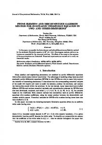
3.2 Traumatic Brain Edema 3.2.1 Neuropathology of Brain Edema Brain edema is a major neurological complication of moderate and severe traumatic brain injury (TBI). It consists of an abnormal accumulation of fluid within the brain parenchyma. Edema and its associated complications account for approximately 50% of deaths in patients with TBI [96]. Traumatic brain edema that frequently accompanies TBIs are either localized around a contusion, or more diffuse. CT scanning is usually the first imaging modality for TBI patients and the brain edema is characterized by a darker density on the image (Fig. 3.4). Vasogenic and cytotoxic edema are the two major types of edema after TBI. Vasogenic edema is due to BBB disruption, resulting in an increased extracellular water accumulation, while cytotoxic edema is defined as an increased intracellular water collection [96]. As the etiology of vasogenic edema is relatively well understood, the treatment is therefore fairly effective. However, the mechanisms of cytotoxic brain edema are still unclear, which makes the treatment of choice inadequate. Research has shown that the brain swelling observed in patients with TBI appears to be predominantly cellular [101]. This makes the clinical treatment of TBI edema more complicated.
Figure 3.4: Axial slices of CT images of two patients after decompressive craniotomy. Localized edema around hemorrhages for Patient 1 (left). Diffuse brain edema for Patient 2 (right). 11
Chapter 3
Craniospinal System and Traumatic Brain Edema
(a) Patient 1.
(b) Patient 2.
Figure 3.5: Reconstructed surface of two patients treated with decompressive craniotomy. By removing part of the bone flap, the brain tissue is allowed to expand outside the skull thereby reduce the ICP. Diffusion Weighted (DW) imaging has been used to distinguish these two different types of edema. A decrease in the ECS as found in cytotoxic edema leads to a decrease in the apparent diffusion coefficient (ADC) since the diffusion of water inside cells is slower. In contrast, vasogenic edema with a larger ECS will increase the mobility of water molecules, thereby leading to a higher ADC value [18].
3.2.2 Management and Treatment of Brain Edema Clinically, local and minor edema may be treated conservatively only by observation, while more extensive edematous areas demand intensive care, where the treatment of choice usually follows evidence-based practice [69, 116]. Monitoring the ICP is an integral part of intensive care treatment following moderate and severe TBI. The longer the ICP exceeds 20–25 mmHg, poor outcome for the patient becomes more obvious [69]. On admittance to hospital, the patient with moderate and severe TBI is placed with the head in a 30-degree elevation aimed at optimizing the ICP, the cerebral perfusion pressure and the venous drainage from the head as well as the pulmonary function [69, 116]. For most severe TBI patients with refractory ICP, decompressive craniotomy (DC) is performed as an ultimate therapy by removing part of the skull bone thereby giving the swelling brain more room to expand. The use of DC has increased substantially in an effort to reduce the ICP following cerebral injury. However, complete consensus on its effectiveness has unfortunately not been achieved among clinicians due to the high levels of severe disability and persistent vegetative state found among the patients with DC [40, 138, 141]. Brain tissue is allowed to expand outside the skull (Fig. 3.5) thus causing axonal stretching which was suggested to contribute to the unfavorable outcome for the patient [40].
12
4 Poroelasticity and Finite Element Modeling (Paper I, IV) 4.1 Governing Equations Brain tissue is modeled as a poroelastic material consisting of an elastic solid skeleton composed of neurons and neuroglia, permeated by the interstitial fluid [79, 128, 134]. The governing poroelastic equations for a fully saturated pore fluid flow are based on conservation of fluid mass for the fluid phase and force equilibrium equations for the solid phase [19, 73]. For the fluid phase, mass conservation gives: dζ + ∇ · q = Qs dt
(4.1)
where Qs is a fluid source and ζ is fluid mass increment caused by either the dilation of the solid skeleton or by the compressibility of fluids in the pores due to pressure changes, q is the fluid flux vector. The interstitial fluid flow was modeled with Darcy’s law, κ q = − ∇p µ where p is the interstitial fluid pressure (IFP).
(4.2)
The final equation governing the fluid phase of a poroelastic material can be written as: ∂p κ ∂ + ∇ · (− ∇p) = −α �b + Qs (4.3) ∂t µ ∂t where S� is the specific storage term, κ is permeability, µ is the fluid viscosity, and �b is the volumetric strain of the solid skeleton. S�
The equilibrium equation for the solid phase gives: G ∂uk ∂p = −α (4.4) (1 − 2ν) ∂xi xk ∂xi where α is the Biot coefficient, G is the shear modulus which for an isotropic material is E related to Young’s modulus E and Poisson’s ratio ν according to G = 2(1+ν) . Note that all the elastic constants in the poroelastic equation are the drained values. − G∇2 ui −
The parameter α can be interpreted as an effective stress coefficient because this coefficient enables the conversion of a multiphase porous medium into a mechanically equivalent 13
Chapter 4
Poroelasticity and Finite Element Modeling (Paper I, IV)
single-phase continuum according to σ 0 = σ + αp [73, 112], where σ 0 is the effective stress added on the solid skeleton, σ is the total stress. For a fully saturated system, it is likely that α should be close to 1. The Skempton coefficient B, representing the ratio of fluid pressure increment and confining pressure pc is defined as [73]: ∂p dpc
B=
!
(4.5) undrained
S� is related to α and B via [73]: S� =
α(1 − αB) KB
(4.6)
E where K = 3(1−2ν) is the bulk modulus of the solid skeleton. S� , represents the amount of interstitial fluid that can be forced into an unchanging volume of parenchyma per unit increase of fluid pressure [91]. The more compliant a system, the value of S� tends to be larger.
The macroscopic level parameters α, B and S� define the solid-fluid system as a “lumped” model. For an ideal isotropic and homogeneous porous media, they are related to the micromechanical ones according to [48, 73]: α=1−
B=
φ( K1f S� =
K Ks
1 − K1s − K1s ) + ( K1 −
(4.7)
1 ) Ks
φ α−φ + Kf Ks
(4.8)
(4.9)
where φ is the porosity, Kf is the bulk modulus of the fluid, Ks is the bulk modulus of the solid grains, which here are the brain cells.
4.2 FE Modelling of the CSF System 4.2.1 FE Modelling of the Human Brain and CSF A Finite Element (FE) model of the adult human head (the KTH head model [84]) has been developed, including the meninges, brain tissue, cerebrospinal fluid (CSF) including a simplified neck with the extension of the spinal cord. The FE mesh used in this study was modified from the KTH head model with addition of aqueduct, foramina of Magendie and foramina of Luschka to construct a fully connected CSF circulation system (Fig. 4.1) [92]. The hexahedral elements in the original KTH head model was split into tetrahedral elements and imported into COMSOL Multiphysics (Comsol Multiphysics, 2010, version 14
4.2 FE Modelling of the CSF System
Figure 4.1: (a) FE head model including the meninges, brain, cerebrospinal fluid (CSF), aqueduct, foramina and neck with the extension of the spinal cord. (b) The CSF circulation system. 4.0a) where all the simulations were performed. Shell elements were used to model the falx, tentorium and spinal dura mater. For both solid and shell elements, 2nd order shape functions were used with a total number of 946488 degrees of freedom (DOF) for the model. The transient infusion analysis was solved using an implicit method; the backward differentiation formula (BDF) which is a standard available method in COMSOL.
4.2.2 Boundary Conditions The outer layer of the solid phase of the CSF is fixed due to the rigid skull constraint. The dura mater surrounding the spinal cord CSF is attached to the simplified neck. The outer surface of the neck is set free since the spinal dural sheath can accept a quantity of CSF as it does not fit the canal closely, being surrounded by a layer of loose areolar tissue and plexus of epidural veins [66] (Fig. 4.2, left). The ventricle wall is set free to move. Fluid pressure inside the ventricle acts as a total pressure p on the ventricle wall which is supported by the solid skeleton (σ 0 ) of the brain tissue and the interstitial fluid pressure (p) inside brain tissue according to −p = σ 0 −αp. For example, α = 1 gives σ 0 = 0 and the pressure will be totally supported by the interstitial fluid in the brain tissue. Otherwise, if α < 1, the ventricle fluid pressure will be supported by both the interstitial fluid and the solid skeleton of brain tissue. At the interface between the simplified non-porous neck and the porous subarachnoid space (SAS), the total stress from the porous SAS was added to the neck (Fig. 4.2, right) shows the choroid plexus in the model where CSF is produced and CSF is absorbed at the SSS and the spinal nerve roots.
4.2.3 Modeling of Normal CSF Dynamics and Infusion CSF is produced mainly at the choroid plexus in the lateral and third ventricles. It flows along the aqueduct of Sylvius to reach the fourth ventricle, and then flows out into 15
Chapter 4
Poroelasticity and Finite Element Modeling (Paper I, IV)
Figure 4.2: Boundary conditions in the FE model. Solid phase boundary condition. Outer layer of CSF (dura) is set to fixed due to the rigid skull constraint. Falx and tentorium edges were set to fixed where it is connected to skull (left). Fluid phase boundary conditions: CSF is absorbed at both arachnoid villi at super sagittal sinus (69%) and at spinal nerve roots (31%) (right). the SAS. CSF flows around the tentorium downwards to the spinal SAS and some flows upwards to the superior sagittal sinus (SSS) where most of it is absorbed by the arachnoid granulations [46]. The rate of CSF production is reported to be at a relatively constant rate. Arachnoid granulations are the major sites where CSF is absorbed into the venous blood, located mainly at the SSS and the spinal nerve roots [50, 57]. They protrude through the dura into SSS and act as one-way valves. As CSF pressure increases, more fluid is absorbed. When CSF pressure falls below a threshold value, the absorption of CSF ceases. In this way, the CSF pressure is maintained at a relatively constant level for healthy human subjects. The model incorporates a balanced CSF production and absorption for the normal CSF circulation system [92]. A constant rate of CSF production Qprod = 0.38 ml/min [94] was defined as Qs in the fluid governing equation (Eq. (4.3)) at the choroid plexus in both the lateral and third ventricles in the FE model (Fig. 4.2). CSF absorption is linearly dependent on the pressure difference between the pressure at the SSS and the venous blood pressure pb (650 Pa) [128] according to: κ µ
∂p ∂xi
!
= Cb (pb − p)
(4.10)
According to the compartment model, the value of outflow conductance (Cb ) can be calculated according to Qprod + Qinf = Cb (PICP 2 − PICP 1 ) [78], where Qinf is the infusion rate and PICP 1 and PICP 2 are the steady state pressures before and during infusion, respectively. A value of 0.10 ml/min/mmHg calculated from experimental data [94] was used. This value is close to the average value of 0.11 ml/min/mmHg reported by [3]. In the model, the absorption occurs at both SSS (69%) and spinal nerve roots (31%) by 16
4.2 FE Modelling of the CSF System splitting Cb proportionally and the value used in the model was adapted according to the selected absorption boundary. With extra fluid injected into the system, Intracranial Pressure (ICP) will be raised thus resulting a higher absorption rate and eventually a new equilibrium state is established at a higher ICP level. Infusion is equivalent to an extra CSF production since the ventricular system is communicating with the SAS. Thus, infusion was modeled as an extra fluid source (Qinf ) added to the normal CSF production rate (Qprod ) and yields Qs = Qinf + Qprod in Eq. (4.3).
4.2.4 Modeling of Gravity and Edema Formation of brain edema involves fluid movement from the vasculature directly into the intracellular space (cytotoxic brain edema) or extracellular space (vasogenic edema) [96]. The circulation of CSF tends to be disturbed for edema patients with high ICP. However, the detailed mechanisms behind edema and disturbed CSF circulation are out of range of this study. A fluid source was used to simulate the extra fluid accumulation. In this model, we consider the influence of gravity on a patient with edema at the posterior part of the brain for the supine and prone positions. The model was based on the normal CSF circulation model with addition of a focal edema at the posterior part of the brain.
17
5 Strain Level Quantification from Image Registration (Paper II, III) A general introduction of image registration will be given first followed by introducing the Diffemorphic Demons (DD) algorithm. From the displacement field obtained from DD registration, the Lagrangian finite strain tensor is derived.
5.1 Image Registration - An Introduction Image registration is to find a spatial transformation that brings one moving image into alignment with a fixed image to a best match [43]. Methods for medical image registration can be divided into those using parametric transformation functions and those using non-parametric ones [4]. The parametric methods are characterized by featuring a transformation function that is described by a quite limited number of parameters, such as rigid and affine transformations. In contrast to parametric registration with only a few parameters needed to be determined, non-parametric methods involve finding a transformation function describing the displacement of the point represented by the voxel, thus usually millions of parameters need to be determined. Unlike a rigid or affine transformation which is a global transformation that applies to the whole domain, non-parametric registration allows to account for more complex shape change, such as local distortion and deformation. Thus, it has found its wide application in clinics such as to guide treatment and monitor disease progression. Non-parametric registration aims at finding a displacement vector of each of the voxels that “best” matches the images together. The goodness of the match is based on a cost function, which is maximized or minimized using some optimization algorithm (e.g. Powell’s Method, Steepest Gradient Descent, Conjugate Gradient Method etc. [43]). Performing the registration is an iterative process that involves transforming the moving image many times by adjusting different parameters until a matching criterion (e.g. the sum of squared differences between the images [4]) is optimized. Non-parametric image registration is an ill-posed problem and is generally with no unique solution which can lead to many displacement fields. A regularization term is needed to guide how the image should be deformed in order to turn the problem to a well-posed problem. Continuum based method, such as linear elasticity [7] and viscosity fluid [36] has been proposed. Demons method was first introduced by Thirion [136] and based on the concept of “demons” that was introduced in the 19th century by Maxwell to illustrate a paradox of thermodynamics. One of the main limitations of the demons algorithm is 19
Chapter 5
Strain Level Quantification from Image Registration (Paper II, III)
Figure 5.1: An example illustrates Diffemorphic Demons registration on binary images with resolution of 750×659. The image on the left depicts the undeformed moving image followed by the deformed moving image (middle 1) and the fixed image (middle 2). The image on the right shows the obtained displacement field result by applying it to a rectilinear grid which drives the moving image to the fixed image. The displacement field is overlayed with the deformed moving image (right).
that it doesn’t provide diffeomorphic transformations1 . As an extension of the demons algorithm, an efficient non-parametric diffeomorphic demons image registration algorithm was proposed which allows a smooth local variation and large deformations [143]. It’s these different physical models that differentiate the non-parametric registration methods from each other. Elastic models treat the source image as a linear elastic solid and deform it using forces derived from an image similarity measure [7]. The image is deformed until the internal force inside the elastic solid is equilibrated with the corresponding external image matching force. This method tends to over-penalize on the displacement thus doesn’t allow large deformation. DD algorithm, on the other hand, allows for large deformation and has been widely used in brain image registration which accounts for large variations between different subjects accounting for the localized deformation [143]. An example illustrates the non-parametric image registration using DD registration algorithm (Fig. 5.1). Image registration has found its wide applications, in functional MRI which align different modality images of the same patient and atlas based segmentation by morphing using probability atlas [30]. Another important application is to track the displacement of the object from one state to another from which the strain level can be quantified noninvasively. This has been used widely to calculate the strain level in the form of the Lagrangian finite strain tensor in different organs such as the lung and heart [21, 52, 59, 59, 62, 114, 144, 145]. Image registration methods has also been used with intra-operative MR images to quantitatively investigate the brain deformation and the approach provides the deformation throughout the entire brain [42, 62–64, 107].
1
Diffeomorphism is a Lie group of invertible and differentiable bijective transformations. A diffeomorphic dense displacement field indicates no tearing or folding in the physical space after deformation [143].
20
5.2 Diffemorphic Demons Algorithm
5.2 Diffemorphic Demons Algorithm The core components of the DD registration algorithm including similarity measures and the regularization model is described here.
5.2.1 Similarity Criterion Given a fixed image F (·) and a moving image M (·), intensity-based image registration is posed as an optimization problem that aims at finding a spatial mapping that will align the moving image to the fixed image. The transformation s(·), RD → RD , p 7→ s(p), models the spatial mapping of a particular point p from the fixed image space to the moving image space [142]. The similarity criterion Esim (F, M ◦ s) measures the quality or the goodness of the matching of a given transformation. In this study, binary images are used, and the sum of the square difference (SSD) suffices for our application as defined in Eq. (5.1). Esim (F, M ◦ s) =
1 X 1 |F (p) − M (s(p))|2 kF − M ◦ sk2 = 2 2Ωp p∈Ωp
(5.1)
where M ◦ s represents the morphed moving image 2 , ΩP is the region of overlap between F and M ◦s. The problem now becomes an optimization problem to find a transformation s over a given space that minimizes the similarity energy function Esim .
5.2.2 Diffeomorphic Demons Model In order to end up with a global minimization of a well posed criterion, the similarity energy function in Eq. (5.1) was modified by introducing an auxiliary variable (i.e. correspondence c) in the registration process [32]. The introduction of this auxiliary variable c decouples the complex minimization into simple and efficient steps by alternating optimization over c and s. Considering a Gaussian noise on the displacement field, the global energy then becomes [142]: E(c, s) =
1 1 1 E (F, M ◦ s) + 2 dist(s, c)2 + 2 Ereg (s) 2 sim σi σx σT
(5.2)
where σi accounts for the noise on the image intensity, σx accounts for a spatial uncertainty of the correspondences and σT controls the amount of regularization that is needed. dist(s, c) =k c − s k and Ereg (s) =k 5s k. The model assumes that so-called “demons” at every voxel from the fixed image are applying forces that push the voxels of the moving image into matching up with the fixed image. The transformation s is driven by a “demons force” derived from the assumption of image intensity conservation [136]. The original demons algorithm has been modified and which allows to retrieve small and large dense displacement field defined as [31]: 2
◦ is the composition operation, M ◦ s means apply the transformation s on the moving image M .
21
Chapter 5
Strain Level Quantification from Image Registration (Paper II, III)
U(p) =
F (p) − M (s(p)) ∇F (p) k ∇F (p) k2 +α2 (F (p) − M (s(p)))2
(5.3)
U(p) is the displacement (corresponding to transformation s as defined in Eq. (5.4)) at point p defined in the fixed image, where α is a positive homogenization factor. The updated unconstrained dense displacement field is computed based on an optical flow computation at each voxel at every iteration. The resulting updated field is added to the global deformation field and the displacement field is regularized by applying a Gaussian smoothing filter. In order to solve the displacement field U, the global energy defined in Eq. (5.2) needs to be minimized. This energy function allows the whole optimization procedure to be decoupled into two simple steps. The first step solves for the correspondence c by optimizing σ12 Esim + σ12 k s − c k2 with respect to c and with s given. The second step solves x i for the regularization by optimizing σ12 k s − c k2 + σ12 Ereg (s) with respect to s and c x T given [143]. The transformation s in the original Demons method [136] is not constrained and doesn’t provide diffeomorphic transformations. A diffeomorphic extension to the demons framework was proposed by adapting the optimization procedure to a space of diffeomorphic transformations. It’s performed by using an intrinsic update step which computes the vector field exponentials of the Lie group of diffeormorphims (see [142] and [143] for details). The displacement field is iteratively updated while introducing elastic regularization by smoothing the deformation field with a Gaussian filter between iterations. The DD algorithm has been fully integrated in the open source software Slicer 3D [115] which was used in this study. The selection of the regularization parameters is crucial in Demons registration. Strong regularization constraints hinder large deformations and provide a poor intensity match. In contrast, parameters leading to a weak regularization do not constrain the deformation enough and often lead to non diffeomorphic results [65].
5.3 Displacement Field and Lagrangian Finite Strain Calculation From the Diffeomorphic Demons registration, the transformation s, corresponding to a displacement field U(X), is obtained from Eq. (5.3). The displacement field is defined on every voxel in the fixed image and morphs the fixed image to the moving image. The strain tensor could then be calculated based on the theory of continuum mechanics (see Appendix: A for more detail). A Lagrangian reference frame was assumed at the fixed image space. s : x = X + U(X)
(5.4)
The displacement field U(X) = [UX , UY , UZ ] for each voxel, obtained from the image registration, gives a reasonable alignment to bring the fixed image at point p with coordi22
5.3 Displacement Field and Lagrangian Finite Strain Calculation nates X(X, Y, Z) to its corresponding point in the moving image at coordinates x(x, y, z) [143]. The displacement gradient is defined as [70]:
grad(U) =
dU = dX
dUX dX dUY dX dUZ dX
dUX dY dUY dY dUZ dY
dUX dZ dUY dZ dUZ dZ
(5.5)
The deformation gradient defined as F=
dx d(X + U(X)) dU = =I+ = I + grad(U) dX dX dX
(5.6)
The Lagrangian finite strain tensor E is defined as E=
� 1� T F F−I 2
(5.7)
The Lagrangian finite strain tensor, E, is a 3×3 symmetric tensor representing the deformation of a point. Different scalar indices can be derived from the tensors, especially the principal strains which represent the maximum and minimum normal strains experienced at a point, are characterized by the tensor eigenvalues. The corresponding eigenvectors reveal the principal strain directions. Thus, they characterize the orientation of the strain. The Jacobian operator can be used to measure local relative volume change. It is defined at the point p as the determinant of the Jacobian matrix of the deformation field as
J = det(F) = det (I + grad(U)) = det
dUX dX dUY dX dUZ dX
1+
1
dUX dY Y + dU dY dUZ dY
1
dUX dZ dUY dZ Z + dU dZ
(5.8)
The determinant of the Jacobian matrix of the deformation field, J, represents the local relative volume. Where J < 1, local contraction is implied, J = 1 implies no volume change and J > 1 implies local expansion [106].
23
6 Water Content Quantification from CT Images (Paper II) Brain edema is a major neurological complication of traumatic brain injury (TBI) commonly including a pathologically increased Intracranial Pressure (ICP) associated with poor outcome. The presence of traumatic brain edema, in its various forms is of great clinical importance and is found to be related to the severity of brain injuries. Although the localized occurrence of edema can be demonstrated by medical imaging techniques, such as Magnetic Resonance (MR) or Computed Tomographic (CT) images, quantification of water content (WC), as is an aspect that could play an important role in the evaluation of the dynamics of brain edema and the monitoring of the efficiency of treatment, is much more demanding. This part of the thesis is concerned with WC extraction from CT images. A brief introduction of WC extraction from medical images including MRI and CT will be given first, followed by CT physics and then the procedures for WC mapping.
6.1 Water Content Extraction from Medical Images - An Overview 6.1.1 Water Content Extraction from MR Imaging MR imaging has been widely used in measurement of WC non-invasively [15, 53, 54, 85, 110] based on the principle that MR signal intensity is proportional to the number of protons in the tissue which in turn is proportional to WC [110]. The image intensity we see directly from the MR images can not be directly related to WC since they are dependent on the scanning parameters. First, different pulse sequences result in different mathematical expressions for signal intensity. Within the same pulse sequences, the image is also influenced by different parameters. T1 or T2 relaxation time, however, is an intrinsic property of the tissue and has been shown to closely relate to WC. T1 or T2 relaxation time map could be obtained by using special protocols and repeat the scanning using different pulse sequence parameters. Evaluation of WC from T1 relaxation time was initialized by Bell et al. from 1980s [15, 54] due to the sensitivity of the T1 relaxation time to WC. The development of a theoretical framework for relating measured relaxation times to WC as well as the validation of the model predictions in a series of phantom and animal studies can be found in [55]. The method has been further studied by several researchers and was found to be a reliable method for the noninvasive characterization of brain edema [55, 100]. T2 relaxation time has also been related to WC in previous studies [53, 95]. 25
Chapter 6
Water Content Quantification from CT Images (Paper II)
Another MR imaging technique, Diffusion Weighted (DW) imaging has also been used to study WC by relating the derived parameter, apparent diffusion coefficient (ADC) with WC. ADC reflects overall diffusivity and a higher ADC is related with a higher WC. Experiments showed a linear relationship between ADC and WC [87, 127].
6.1.2 Water Content Extraction from CT Image Although WC extraction from MR imaging has shown very promising results. For severe TBI patients, however, MR scanning is not recommendable for unstable patients. Furthermore, using this method, MR scanning needs to be repeated with different pulse sequence parameters to obtain the relaxation times and special protocols are needed thus reducing its clinical application. CT imaging, however, is usually the first imaging modality for TBI patients [69, 90]. Therefore, this part of the thesis explores the possibility of quantifying WC from CT images in order to evaluate the progression or regression of brain edema for patients treated with decompressive craniotomy. WC of the edematous brain is one of the major determinants of CT attenuation. Hounsfield unit (HU) value from CT image has been reported to be closely related to WC [74, 119, 121]. Measuring CT attenuation allows localization and quantification of edema as well as study of sequential tissue changes in the living brain when correlated with pathological specimens [119]. The HU value from CT image is closely related to the severity of brain edema which appears as low-density areas on CT images due to excess water accumulation [74, 119, 121]. The HU value was found to decrease linearly when the tissue water is elevated. In regard to ischemic brain edema, with each 1% increase in tissue WC, attenuation will decline by approximately 2 HU [74] which give the relative variation of WC with HU values. Although the aforementioned studies give the relative change of WC based on changes of HU values, the absolute WC is of greater clinical importance for the evaluation of brain edema dynamics. However, the relationship between the absolute WC and HU value from CT images, hasn’t been studied previously.
6.2 CT Physics The approach presented here depends heavily on HU values from CT images. Therefore, for the sake of completeness, a short description of CT principles will be given before the quantitative WC mapping procedure is described.
6.2.1 X-ray Attenuation and HU Value CT imaging is created by directing X-rays at an object from multiple orientations and measuring the resultant decrease in intensity. The intensity is characterized by Beer’s Law, which describes intensity reduction as a function of X-ray energy, path length, and material linear attenuation coefficient. A specialized algorithm is then used to reconstruct the distribution of X-ray attenuation in the volume being imaged [29, 80]. When an X-ray beam with initial intensity of I0 is focused on a subject, the approaching X-rays are either scattered, absorbed or transmitted through the subject, and the intensity 26
6.2 CT Physics of the transmitted X-ray denoted by I is measured by the detector [33]. Consider the case of a monoenergetic photon X-ray passing through a slice of tissue with the attenuation coefficient µi . The output intensity I is given by: I = I0 exp
" X
#
− (µi xi )
(6.1)
i
where xi is the distance traveled by the X-ray beam [49]. The linear attenuation coefficient for the energy spectrum of a typical diagnostic X-ray beam for air, bone, muscle, blood and water are: µair = 0, µbone = 0.48 cm−1 , µmuscle = 0.18 cm−1 , µblood = 0.178 cm−1 , µwater = 0.195 cm−1 [29]. This clearly shows that the linear attenuation coefficient µ is dependent on the material of interest, i.e, the chemical composition. However, note that the linear attenuation coefficient of a material µ is also dependent on the X-ray energy. A higher energy will usually result in a lower µ value [16, 51]. Clinically, CT images are produced with highly filtered, higher-kV X-ray beams with an average energy of 75 keV. At this energy in muscle tissue, photoelectric and Compton scattering account for the majority of the attenuation encountered. About 90% X-ray attenuation is due to Compton scattering and 10% due to photoelectric absorption. Therefore, HU values and hence CT images receive their contrast mainly from the physical properties of tissue that influence Compton scattering [29]. The monochromatic total energy attenuation coefficient µ(E) is a summation of the attenuation due to Compton scattering µc (E) and photoelectric absorption µp (E) defined as [26]: µ(E) = µc (E) + µp (E)
(6.2)
The attenuation coefficient is a function of X-ray energy (E) Eq. (6.2). Given a material with known chemical composition, one can possible to get the attenuation coefficients µ, µc , µp from the mass attenuation coefficients and mass energy-absorption coefficients table [16]. The total mass attenuation coefficients for a mixture could be obtained by adding the coefficients for each element weighted by the compositions fraction [16, 26]. A more complete table for mass attenuation coefficients for element media, compounds and mixtures can be found in [72]. HU values provide information on the X-ray attenuation characteristics of the material relative to that of water (µw ) [26, 29] which is defined as: HU = 1000(µ − µw )/µw
(6.3)
Accordingly, the HU value for air should be -1000 and 0 for water in the absolute HU scale. Hc and Hp describe the Compton and photoelectric coefficients in exactly the same way as HU describes total attenuation according to [28]: Hc = 1000(µc − µcw )/µcw , Hp = 1000(µp − µpw )/µpw
(6.4) 27
Chapter 6
Water Content Quantification from CT Images (Paper II)
Figure 6.1: An axial and sagittal section from a patient CT image. Before gantry correction, seriously distortion is seen in the sagittal plane (left). After gantry correction, the distorted image is corrected (right).
6.2.2 Image Reconstruction of Attenuation Coefficient By changing the angles of the X-ray photons, CT scanners record “projection” measurements of the transmission of X-ray photons through an object [51] which provides the information of the linear attenuation coefficient for the whole domain of interest. Several reconstruction algorithms have been developed to solve the individual linear attenuation coefficient for each point of the matrix including backprojection method, iterative reconstruction, Fourier reconstruction etc. [49]. Image reconstruction has a fundamental impact on image quality and therefore on radiation dose. For a given radiation dose it is desirable to reconstruct images with the lowest possible noise without sacrificing image accuracy and spatial resolution [150].
6.2.3 CT Scan Parameters During the CT scan, radiologists need to balance image quality and dose by selecting appropriate scan parameters and dose reduction methods to be used during scan data acquisition [151]. The most commonly used parameters which need to be adjusted are listed: • Gantry angle. Gantry-tilted CT scanning is used to avoid unnecessary exposure to the vulnerable tissues such as the eyes [93]. If the gantry angle is not zero, the images are distorted. A gantry correction is needed in order to get a correct geometry. By applying an affine transformation matrix with a correct shear factor according to the gantry tilt direction, the image will be corrected. An example shows the image before and after gantry correction in Fig. 6.1. • Tube voltage (kV). Different voltage generates X-ray with different energies and energy spectra [81]. The maximum energy of the generated X-ray photon in kiloelectron volt (keV) is numerically equal to the applied kilovolt peak (kVp). Most CT scanners have a limited range of kVp choices when performing CT scans. Routine body CT for adult patients is generally performed at 120 to 140 kVp. The use of 80 kVp is a widely accepted level when attempting to reduce radiation doses in pediatric patients [5]. 28
6.3 Water Content Extraction • X-ray tube current (mA) and exposure time (ms). X-ray tube current (mA) controls the X-ray intensity. The tube current (mA) is usually adjustable over a wide range from 10 mA to 800 mA. The effect of tube current (mA) on image quality is more straightforward than that of tube voltage (kV) [5]. • Reconstruction kernels. Different reconstruction kernels such as “soft”, “standard”, “soft tissue” have been used in order to get a better contrast for different types of tissues, which are also called “convolution kernels”, since this act as a filtering function. The raw data are mathematically filtered before being backprojected (one method for image reconstruction) onto the image matrix. This involves convoluting the projection data with a convolution kernel. Different kernels are used depending on the clinical applications such as soft tissue imaging or bone imaging. Bone kernels have less high-frequency roll-off and hence accentuate higher frequencies in the image at the expense of increased noise [20].
6.3 Water Content Extraction The extraction of WC is based on a relationship between WC and specific gravity (SG) [111], and SG could be obtained from the HU in the CT images by a photoelectric correction value 4Hp [26, 27, 119] according to the chemical composition and the X-ray energy. SG then serves as a bridge to connect the HU value from CT image with that of the WC. In order to make the HU values from different images comparable, both pre- and post-craniotomy images were calibrated using a two-point calibration method using CSF and air as references [22]. Different equations apply for gray and white matter due to the chemical composition difference which makes it necessary to segment the images. This was performed by using an atlas based method [30]. Morphing a segmented brain atlas to the patient brain according to the cranial and lateral ventricle shape and the morphed template gives the segmented image. This section will discuss the relationship between SG and its relation to WC. SG is related to the HU values from CT images. Based on this, the relation between WC and HU values from the CT images could be established.
6.3.1 HU Value and Specific Gravity SG and HU value SG is the ratio of the unknown density to that of water which is defined according to [28, 119] SG =
n ρe nw ρew
(6.5)
where n is the number of nucleons per electron which can be calculated according to the chemical formula of the material. For water, nw = 1.8015. ρe is the electron density with unit of electrons/cm3 . The electron density ρe is defined as ρe = ρN (Z/A)ef f , where Z is the effective atomic number, A the effective atomic mass, N is Avogadro’s number (6.023e23, a constant), ρew is the electron density of water, and ρ is the density [126]. 29
Chapter 6
Water Content Quantification from CT Images (Paper II) %H
%C
%N
%O
%Na
%P
%Cl
%K
White matter
10.56
17.80
1.88
68.72
0.124
0.434
0.124
0.36
Gray matter
10.58
10.09
1.79
76.46
0.15
0.35
0.15
0.43
Table 6.1: Chemical composition of cerebral white and gray matter [27]. The percentage is the weight fraction of each of the elements.
The Compton scattering is proportional to electron density, and the electron density of the material can be related to Hc according to [28, 119]: ρe /ρew = (1 + Hc /1000)
(6.6)
Combining Eq. (6.6) with Eq. (6.5) leads to [28, 119]: SG = n/nw (1 + Hc /1000)
(6.7)
The HU value is related to Hc by a photoelectric correction 4Hp according to [28, 119]: Hc = HU − 4Hp
(6.8)
For a material with known chemical composition, the value of HU and Hc can be calculated from the mass-attenuation coefficients and the photoelectric correction value 4Hp can then be calculated. In this way, the SG value is related to the HU value from the CT images. Photoelectric correction (4Hp ) for gray and white matter The chemical composition of cerebral white and gray matter listed in Table. 6.1 are taken from [27]. The CT machine generated X-ray spectrum is usually poly-energic. Images obtained at a tube voltage of 120 kVp corresponds to an effective energy of approximately 70 keV [102]. µc /ρ is the Klein-Nishina function for Compton scattering (Incoherent scattering) and it represents the photoelectric absorption, which also includes the coherent scattering binding energy corrections [26, 27]. The values of the mass attenuation coefficients µc /ρ, µp /ρ for the elements found in brain tissue at 70 keV was obtained from the Photon Cross Sections Database which provides mass attenuation coefficients for all of the elements Z = 1 to 92, and for compounds and mixtures of radiological interest [16] as listed in Table. 6.2. According to the weight fraction of the elements for gray and white matter from Table. 6.1, the total mass attenuation coefficients were calculated by adding the coefficient of each element weighted by the composition fraction listed in Table. 6.3. In order to get the linear attenuation coefficients, a density value for normal gray and white matter is needed which are ρ = 1.0433 g/cm3 for gray matter and ρ = 1.0398 g/cm3 30
6.3 Water Content Extraction H
C
N
O
Na
µc /ρ(cm2 /g)
0.3167
0.1565
0.1559
0.1554
µp /ρ(cm2 /g)
0.000565
0.0107
0.0155
0.0218
P
Cl
K
0.1466 0.1457
0.1431
0.1439
0.0510
0.1885
0.2695
0.1297
Table 6.2: Mass attenuation coefficients of the elements of the brain tissue at 70 keV. WM
GM
Water
µc /ρ (cm2 /g)
0.1725
0.1724
0.1734
µp /ρ (cm2 /g)
0.0191
0.0201
0.0194
µ/ρ
0.1916
0.1925
0.1928
Hc
34.45
37.33
-
Hp
20.70
77.09
HU
33.07
41.34
4Hp
-1.386
4.0098
Table 6.3: Calculation of 4Hp for gray matter and white matter.
for white matter, respectively [23]. The mass attenuation coefficients in Table. 6.3 were then converted to linear attenuation coefficients by multiplying the density. The value of Hc and Hp and HU are calculated according to Eq. (6.3) and Eq. (6.4) with the results listed in Table. 6.3.
6.3.2 Relationship between Specific Gravity and Water Content WC is defined as: %W C = (Wt − Wd )/Wt × 100
(6.9)
Where Wt is the weight of the fresh tissue, Wd is the dried weight. The relationship between SG and WC is related according to [99, 111]: W C = (m(1/SG) + b) × 100
(6.10)
The slope m = SGs /(SGs − 1), and intercept b = 1/(1 − SGs ). Where SGs is the SG of the tissue solids. SG relates to the relative WC of the tissue. Based on the experimental values obtained by Marmarou et al. [98, 99], an equation relating SG and WC for both gray and white matter could be established. The average measured SG is 1.146 for white matter, and 1.26 for gray matter. Using these constants, the final equations relate WC to SG values in an abbreviated form as following: W CW M = 784.93/SG − 684.93
(6.11) 31
Chapter 6
Water Content Quantification from CT Images (Paper II)
W CGM = 484.62/SG − 384.62
(6.12)
According to the above equations, the calculated WC for normal gray matter is 79.89% (SGGM = 1.0433), and WC for normal white matter is 69.93% (SGW M = 1.0398). These values correspond well with the reported values from the literature with values of 79.7% for gray matter and 69.9% for white matter [54].
6.3.3 Calibration of the HU Values from CT Images using Air and CSF as References Two-point calibration of HU values using CSF and air as references It’s difficult to correlate HU values from one investigation to another and from one CT scanner to another. There are many factors affecting the reconstructed linear attenuation coefficient µ and the HU value showing on the CT images, especially since µ is energy dependent. Other factors include short and long term changes in X-ray dose, instability of the detector system and calibration error of the detector system in relation to water. In order to convert the HU values to a true HU scale (H w = 0; H a = −1000), a two-point calibration using air and water was proposed [28] according to Eq. (6.13): HU = 1000(Hm − Hw )/(Hw − Ha )
(6.13)
where Hm is the measured Hounsfield value reading from the CT images. In clinics, however, CSF instead of water, has been used as reference [22] in order to make the HU values from different CT images comparable. In this work, we used a slightly modified equation using CSF and air as references according to ¯ ¯ CSF + (Hm − Hm_CSF ) ∗ (−1000 − HCSF ) HU = H (H m_air − Hm_CSF )
(6.14)
¯ CSF is the average HU value of CSF in the two set of images to be compared where H (e.g. pre- and post craniotomy images). It’s important to make this calibration since this will not only allow to make the HU value differences meaningful, but also the absolute HU value. Convert the measured HU values to the true HU scale using CSF and air as reference A series of ROI was manually selected in different slices at the voxels where it’s purely CSF. Totally 24 ROIs were selected and the same procedure was made for ROIs of air. It’s necessary to avoid the places with metal streak artifacts and select only the areas which is pure air. The mean HU value of CSF for different CT images were summarized Table. 6.4. 32
6.3 Water Content Extraction Patient 1
Patient 2
CSF
air
CSF
air
Precraniotomy
5.5217
-999.4390
4.8060
-997.7925
Postcraniotomy
1.9581
-998.9121
2.3675
-1.0001e+03
Average
3.7399
-
3.5868
-
Table 6.4: Mean values for CSF and air in pre and post-craniotomy scans for two TBI patients . WM
GM
SG = 1.006(1 + (HU − (−1.3860))/1000) SG = 1.006(1 + (HU − 4.0098)/1000) W C = 784.93/SG − 684.93 W C = 484.62/SG − 384.62 Table 6.5: Final equations relating HU values with water content for gray and white matter.
From the result in Table. 6.4, the HU value for air is very close to -1000, and the HU value for CSF is between 2 - 6 which is very close to the value obtained in [22] which is between 2 and 4 for infants from 0-5 years of age. Other reported values lies in between 0 - 10 [71]. This indicates that the CT scanner should have already been calibrated to fit the HU scale.
6.3.4 Relationship between HU Values and Water Content After the HU value from the CT images has been calibrated using the procedure described in Section 6.3.3, the WC could then be directly related with HU values using the final equations listed in Table. 6.5.
6.3.5 Segmentation of Gray and White Matter As different equations apply for gray and white matter, it is necessary to segment the gray and white matter. The common CT image segmentation is based on the gray values determined by the HU values. The HU value differences makes the CT image darker for white matter then for gray matter. However, due to the lack of clearly defined edges, segmenting these structures remains a challenging task that will not be accomplished by designing algorithms that rely solely on information present in the image but also a priori information is needed [47]. This is especially difficult for the CT image of edema patients where the WC variation already changes the HU values. We used a template based method. First the MRI image from a normal brain with similar age was segmented using probability map as a priori information combined with expectation-maximization (EM) algorithm method using the open source software Slicer3D [115]. The ventricle and cranial shapes were used to morph to the pre- and post-craniotomy stage. The morphed segmented gray and white matter of the normal MRI is the segmented image for the 33
Chapter 6
Water Content Quantification from CT Images (Paper II)
Figure 6.2: CT image and the segmented results for Patient 1 evaluated at precraniotomy (upper row) and Post-craniotmy (lower row) .
Figure 6.3: CT image and the segmented results for patient 2 evaluated at Precraniotomy (left column) and Post-craniotmy (right column).
34
6.3 Water Content Extraction patients with the results showing in Fig. 6.2 and Fig. 6.3 for Patient 1 and Patient 2, respectively.
35
7 Fiber Tractography from Diffusion Weighted Imaging (Paper III) Diffusion Weighted (DW) Imaging, is a Magnetic Resonance (MR) technology that noninvasively measures the random motion of hydrogen atoms within water molecules in all three dimensions. After its development it has found wide applications in clinics. It’s capable of detecting subtle abnormalities in various of diseases such as stroke, multiple sclerosis, dyslexia, and schizophrenia [89]. Different indices derived from DW images have been found to provide more information of traumatic brain injury (TBI) patients which is usually invisible when using other MR imaging techniques [24, 122]. From DW images, diffusion tensor could be derived based on which fiber tractography can be extracted representing the white matter fiber bundle connections in the brain. Fiber tractography has been used for tumor resection surgery planning in order to get around the most important fibers in the brain. Fiber tracts contribute to the anisotropic properties of brain tissue and the orientations of fiber tracts have been integrated in biomechanial modeling which are of great importance to have more insight into the axonal injuries [34, 38, 39, 149]. In this chapter, the basic principles of DW imaging will first be given followed by diffusion tensor analysis, and finally a method to extract fiber tracts is described.
7.1 Diffusion Physics The random movement of particles suspended in a fluid or gas is refereed to as a Brownian motion. In a homogeneous, barrier-free medium, provided that the number of molecules is sufficiently large, the squared diffusion displacements r, averaged over all the molecules in the ensemble, is directly proportional to the observation time τ . In n dimensional space: r2 = 2nDτ, n = 1, 2, 3
(7.1)
where r2 is the mean squared displacement of the molecules. The scalar proportionality constant D is known as the diffusion coefficient and depends on the medium viscosity, the particle size and the temperature [68]. Consider, for example, pure water which is known to have a self-diffusion coefficient of approximately D = 3 × 10⁻³ mm2 /s at body temperature (37o ). If water molecules are followed to diffuse freely in three dimension, the displacement over an interval, say τ = 50 ms 1 , the square root of r2 according to Eq. (7.1) is 0.03 mm. The resultant distance water molecules migrate, if they were free, is much greater than the cellular dimension [35]. Thus, when water molecules migrate in 1
Represents the measurement interval commonly used for in vivo diffusion imaging procedures.
37
Chapter 7
Fiber Tractography from Diffusion Weighted Imaging (Paper III)
the brain tissue, it’s inevitable that the water molecules will be hindered by the axonal membranes and the myelin sheaths. Diffusion is said to be isotropic when the displacement due to Brownian motion is directionally independent. In this case, a scalar value D is sufficient to represent the diffusion characteristic in brain tissue, such as gray matter, where the measured apparent diffusivity is largely independent of the orientations of the tissue. However, in white matter, for example, the diffusivity is dependent upon the orientation of the tissue. No single scalar can characterize the orientation-dependent water mobility in these tissues. Instead, a symmetric effective or apparent diffusion tensor is needed in such cases [9, 88].
7.2 Diffusion Weighted Imaging and Diffusion Tensor Analysis 7.2.1 Diffusion Weighted Imaging From a series of DW images, the effective diffusion tensor, D, can be estimated using the relationship between the measured signal intensity at each voxel and the applied magnetic field gradient sequence [9, 12]. The diffusion tensor is symmetric (i.e. Dij = Dji ), thus it contains only six unique values. Given this, at least six non-collinear diffusion gradient directions are required to determine the diffusion tensor [10, 35]. In order to improve the quality of the diffusion tensor calculation, a larger number of non-collinear diffusion gradient directions should be used which gives an “over estimation” for the diffusion tensor. In this case, different methods exist to solve the diffusion tensor, such as least square and weighted least square. For detailed theory about DW imaging (see [9, 10, 12, 89] for more detailed information on DW imaging).
7.2.2 Diffusion Tensor Analysis Once the diffusion tensor D is determined, different indices can be derived to provide information for each voxel in the image. The diffusion tensor is a real, symmetric second order tensor. Mathematically, this entails a linear rotation of the diffusion tensor to diagonalize it thereby setting off-diagonal elements to zero [89].
Dxx Dxy Dxz λ1 0 0 D = Dyx Dyy Dyz = [e1 e1 e3 ] 0 λ2 0 [e1 e1 e3 ]T Dzx Dzy Dzz 0 0 λ3
(7.2)
where λ1 , λ2 and λ3 are eigenvalues (λ1 > λ2 > λ3 ) and the corresponding eigenvectors are e1 , e2 , e3 . The eigenvalues of the diffusion tensor provide diffusion coefficients along the orientations defined by its respective eigenvectors [89]. λ1 represents the greatest diffusion value along a fiber axis, denoted by the direction vector e1 . λ2 , λ3 represent the diffusion value along two axes perpendicular to e1 . Because D is symmetric and positive definite, its three eigenvectors (principal coordinate directions) e1 , e2 , and e3 are orthogonal [11]. 38
7.3 Fiber Tractography A number of rotationally invariant scalar parameters can be extracted from the diffusion tensor. The apparent diffusion coefficient (ADC) along any direction g can be calculated according to: ADCg = gT · D · g = λ1 (g · e1 )2 + λ2 (g · e2 )2 + λ3 (g · e3 )2
(7.3)
The Mean Diffusivity (MD), representing the average diffusion in a voxel, can be calculated as the mean of the eigenvalues of diffusion tensor, D. MD is equivalent to the average of three ADCs measured in three orthogonal directions [8] which is defined as: λ1 + λ2 + λ3 ¯ Dxx + Dyy + Dzz = =λ 3 3 ¯ is the mean of the eigenvalues of the diffusion tensor. where λ MD =
(7.4)
The Fractional Anisotropy (FA) is the most commonly used anisotropy measure and is a normalized expression of the tensor eigenvalues [8] according to Eq. (7.5).
FA =
v � �2 � �2 � � �2 � u u ¯ ¯ ¯ 3 + λ − λ + λ − λ λ − λ u 3 2 1 t
2 (λ21 + λ22 + λ23 )
(7.5)
FA approaches 0 for perfectly isotropic (λ1 = λ2 = λ3 ) conditions and FA = 1 for perfectly anisotropic tensors (λ1 � λ2 , λ3 ). For example, for white matter of the corpus callosum, which is known to be rich of fiber bundles of the brain, FA ≈ 0.7 − 0.8 [35].
7.3 Fiber Tractography Once the fractional anisotropy (FA) and the preferred diffusion direction has been created, it is possible to perform fiber tracking or diffusion tensor tractography. Streamline
Figure 7.1: Extracted axonal fiber tracts (left). Axonal fiber tracts with three eigenvectors of the diffusion tensor, i.e., axonal fiber orientation (N1 ), and two perpendicular vectors, N2 and N3 (middle). A magnified picture shows the eigenvectors of the diffusion tensor (right). 39
Chapter 7
Fiber Tractography from Diffusion Weighted Imaging (Paper III)
tractography is one of the methods for fiber tract estimation [104, 105]. Streamline tractography uses the maximum orientation described by the eigenvector e1 associated with the largest eigenvalue λ1 , as an estimate of local tract orientation. It assumes that λ1 associated with the maximum eigenvector is the main fiber direction. DW images were performed at a 3D scanner (Siemens Trio-Tim, Erlangen, Germany) acquired with a repetition time of 5.2 s, an echo time of 91.4 ms, b value of 1000 s/mm2 and a resolution of 2 × 2 × 3.6 mm for an image size of 184 × 232 × 151. T1 Weighted images were taken at the same time on a healthy volunteer with the approval of the local ethics committee. The DW images were taken using 30 gradient directions and the diffusion tensors were estimated from the DW images using a standard least square method implemented in the open source software Slicer 3D which provides a comprehensive tool for DWI and diffusion tensor processing [115]. The final extracted white matter tractography using the streamline method [13, 104, 105], contains the polylines (Fig. 7.1, left) with the corresponding diffusion tensor at each fiber point (Fig. 7.1, middle). The major eigenvector of the diffusion tensor, λ1 with its corresponding eigenvector N1 is associated with the tangent to the fiber path and the two other eigenvectors, λ2 and λ3 (N2 and N3 ) are directly perpendicular to the fiber path (Fig. 7.1, right).
40
8 Results The main results from the individual studies will be presented separately.
Results of Paper I : Influence of gravity for optimal head positions in the treatment of head injury patients In Paper I, gravitational force was suggested to have a significant impact on the pressure of the edema zone in the brain tissue. A Finite Element (FE) model including the meninges, brain tissue and a fully connected cerebrospinal fluid (CSF) system was used in this study. Brain tissue was modeled as a poroelastic material consisting of an elastic solid skeleton composed of neurons and neuroglia, permeated by interstitial fluid. Falx and tentorium, formed by the dura mater, was modeled with shell elements. The model includes the CSF generation at the choroid plexus present in both the lateral and third
Figure 8.1: Gravity effects on edema located at the posterior part of the brain. a Pressure distribution for supine (upper) and prone (lower) position in the model. b IFP (upper) and water content increment (lower) distribution along the white matter for both the supine and prone positions. 41
Chapter 8
Results
ventricles, and absorption through arachnoid villies at the superior sagittal sinus (SSS) and the spinal nerve roots (see Chapter 4 for modeling details). To better understand the influence of gravity, modeling of the normal CSF circulation is a prerequisite. Therefore, normal CSF circulation both with and without gravity were simulated first. In the model of normal CSF circulation without gravity, the Intracranial Pressure (ICP) ranges between 1,070-1,097 Pa, which is within the normal range for healthy adults. When gravity was added to the model, pressure was higher at lower parts of the brain in the gravity direction for both the supine and prone positions. This indicates that hydrostatic pressure due to gravity affects the pressure distribution under normal CSF circulation state. The normal CSF model served as a baseline model for the subsequent edema model. The effect of head positions (supine and prone position) due to gravity was investigated for a localized brain edema at the posterior part of the brain. Results from the model showed a higher localized interstitial fluid pressure (IFP) at the edema zone due to extra edema fluid accumulation for both positions (Fig. 8.1 a). However, the average IFP in the edema zone decreased around 15%, from 3,331 Pa to 2,824 Pa, when changing from the supine to prone position. For the supine position, the IFP decreased from the edema zone the whole way to the frontal part of the brain. For the prone position, the IFP at tissue adjacent to the edema showed a similar tendency as for the supine position. However, IFP started to increase at a certain distance (Fig. 8.1 b upper) from the edema zone due to hydrostatic pressure induced by gravity. The tissue pressure gradient forces the interstitial fluid away from the edematous zone to other parts of the brain. When IFP increases, the brain tissue is swelling due to the pressure gradient acting on the tissue skeleton. The predicted water content increment is about 10% at the centre of the edema and decreases towards other areas of the brain (Fig. 8.1 b). The value of water content increment is nearly identical for both positions.
Results of Paper II: Increased strain levels and water content in brain tissue after decompressive craniotomy In Paper II, stretching of brain tissue and the water content (WC) were investigated as these are of significant importance to evaluate and understand the consequences of patients treated with decompressive craniotomy (DC). Two patients were included in this study. The stretching of brain tissue was quantified retrospectively based on the Computerized Tomography (CT) images of the patients before and after DC by a nonlinear image registration method presented in Chapter 5. WC was related to specific gravity (SG), which in turn was related to the Hounsfield unit (HU) value in the CT images by a photoelectric correction according to the chemical composition of the brain tissue. The detailed procedures for WC quantification can be found in Chapter 6. Only the results for Patient 1 is presented here. The results for Patient 2 can be found in appended Paper II. 42
Results
Figure 8.2: Procedures and results of displacement field analysis.
Figure 8.3: Displacement and strain level of the brain tissue in areas abutting the skull base for Patient 1. Displacement magnitude (left). 1st Principal strain (right).
43
Chapter 8
Results
Displacement field analysis To quantify the Lagrangian finite strain tensor, a first step is to calculate the displacement field. The procedures and results for displacement field analysis is presented in Fig. 8.2. The reconstructed surfaces of the segmented binary images are shown in Fig. 8.2 (left column). A representative slice is presented to illustrate the registration results in Fig. 8.2 (middle column). Before Diffemorphic Demons (DD) registration, there is a large discrepancy between the overlayed images around the ventricles. After DD registration, the discrepancy is nearly invisible indicating a good alignment, and the structural change of brain tissue occurring between different stages was accurately captured. From the DD registration, a 3D matching field (displacement field) was obtained which represents the motion of the brain tissue in order to deform the brain shape from one stage to another (Fig. 8.2, right column). Strain level quantification The DC initiated an external motion of the brain tissue and with displacements up to 16 mm (Fig. 8.3, left). In contrast, the maximum strain level was localized around the skull edge of the DC indicating that the neurons in this area were under serious stretching (Fig. 8.3, right). The strain level was quantified in the entire brain tissue with results presented in Fig. 8.4 (upper row). In the pre-craniotomy brain, the strain level is large around the ventricular system which makes the neurons around the ventricles either stretched or compressed (Fig. 8.4, Pre-Craniotomy). Following DC, the strain level increased substantially at the treated side compared to that before the treatment (Fig. 8.4, Post-Craniotomy). The strain level in the central region has increased further up to over 80% around the ventricular wall. Also, the strain is more widespread compared to the pre-craniotomy. Moreover, an increase in strain level on the opposite side of the DC was also observed, however, to a much lesser extent compared to the treated side. The strain can be further analyzed by plotting the strain along the cross-lines before and after DC (Fig. 8.4, a – c) showing the significant influence of the treatment on the strain level. The increased strain level differs significantly depending on where the analysis is taking place. The strain level in the vicinity of the DC shows a higher level after treatment (Fig. 8.4, a and b), while other areas with a longer distance from the DC presents an increase in strain level, to a lesser extent (Fig. 8.4, c). Water content quantification In comparison to normal conditions of WC, which is around 70% for white matter and 80% for gray matter [54], the WC shows a slightly increased concentration in the brain tissue of the traumatic brain injury (TBI) patient after DC (Fig. 8.5, upper row) reaching a WC of up to 90 percent in some areas of the brain tissue. When comparing the WC before and after treatment, the increased WC is more obvious in the white matter of the frontal lobe where a hemorrhage was seen from the CT image. For other parts of the brain, the increased WC is distributed in a relatively similar way in both hemispheres regardless of the area of DC. A probability density function (PDF) was used to depict the 44
Results
Figure 8.4: Strain distribution at a representative axial slice in the healthy, precraniotomy and post-craniotomy period (upper row). Evaluation of the increased strain levels before and after treatment along the crossline in three different areas of the brain tissue (a, b, c, lower row).
45
Chapter 8
Results
7 6
Pre_Craniotomy
Probability Density
Post_Craniotomy 5 4 3 2 1 0 50
55
60
65
70 75 80 CT Measured Water Content (%)
85
90
95
100
Figure 8.5: Quantitative water content (WC) maps for 4 consecutive transverse slices through the brain in the pre-craniotomy (upper row) and post-craniotomy (lower row) period for Patient 1. The probability density function (PDF) of WC for the entire brain shows a shift of WC toward a higher level in the post-craniotomy period. relative frequency at a given water content level. The PDF provided a profile of water content distribution of the entire brain which was characterized by two distinct peaks, one for white matter and one for gray matter (Fig. 8.5). The development of edema is characterized by more voxels at higher water content which is equivalent to a shift of the profile to the right. The average WC in the whole brain is significantly increased after the DC compared to that seen before the treatment (Fig. 8.5). The average WC of the white matter had increased (p < 0.001) from 70.6% ± 5.7% to 73.1% ± 5.9%, and for grey matter (p < 0.001) from 82.5% ± 3.6% to 84.5± 5.9%, respectively (mean ± standard deviation).
Results of Paper III: Decompressive craniotomy causes significant increase of strain in axonal fibers 1st Principal strain at axonal fibers for both the pre- (Fig. 8.6, left, Pre-Craniotomy) and post-craniotomy stage (Fig. 8.6, left, Post-Craniotomy) are presented. For the pre46
Results
Figure 8.6: Displacement and 1st Principal strain at axonal fibers with the values plotted for the fiber points at the region of the treated part.
craniotomy stage, due to the compression of the ventricles, the fibers surrounding the ventricles were most seriously distorted and the strain level at a longer distance to the ventricle is less pronounced. The strain distribution patterns changed after DC. The strain level in the vicinity of the DC shows a higher level after the treatment. A magnified image shows the displacement and the strain of the fibers for both the pre- and postcraniotomy period (Fig. 8.6, right). Greatest axonal fiber displacement of up to 12 mm was found at the treated part of the craniotomy (Fig. 8.6, right, upper). It’s seen that the average 1st Principal strain at these axonal fibers is around 0.3 with a maximum value around 0.49 (Fig. 8.6, right, lower). The evaluation of axonal stretching at the treated part of craniotomy is of great interest since it’s suggested to contribute to the unfavorable outcome for the patients [40, 131]. Thus, strain levels at two representative regions of the axonal fibers at the treated part are plotted to illustrate more clearly how these different strain measures differ from each other (Fig. 8.7). Region 1 was selected at the place where the axonal fibers are close to the skull edge, while region 2 is further away from the skull edge. 1st principal strain is always with the largest value among all strain measures which should be expected. Generally, the axonal effective shear strain is smaller than the axonal strain, however, this is not always the case. At some fiber points, the axonal effective shear strain is indeed larger than axonal strain. 1st principal strain was found up to 0.34 at some point at region 1, with an axonal strain of 0.28 and axonal effective shear strain of 0.12 at the same point. For region 2, the maximum corresponding strain levels are 0.2, 0.17 and 0.06. The axonal effective shear strain at region 1 is much higher than in region 2 representing a larger “tearing” effect to the axonal fibers due to the skull edge. At region 2, the axonal strain is close to 1st principal strain indicates that the axonal orientation at these points is close to the maximum stretching direction (i.e. 1st principal strain direction). 47
Chapter 8
Results
Figure 8.7: Strain levels at the two regions of the selected axonal fibers points. The horizontal axis is the fiber point index (Id), and the strain values vary as a function of the location in the axons. Strain levels at axonal fiber tracts at region 1 (right, upper). Strain levels at axonal fiber tracts at region 2 (right, lower).
Results of Paper IV: Influences of Brain Tissue Poroelastic Constants on Intracranial Pressure (ICP) during Constant-Rate Infusion In Paper IV, the influences of brain tissue poroelastic constants on ICP during constantrate infusion were investigated. Basically, the same FE model was used as in Paper I. However, more poroelastic parameters are required in this study for a transient procedure. Due to a substantial variation in previously used poroelastic constants, the influence of the main poroelastic parameters including the Biot coefficient α, Skempton coefficient B, drained Young’s modulus E, Poisson’s ratio ν, permeability κ, CSF absorption conductance Cb , and external venous pressure pb was studied to investigate the influence on the time-pressure response. A normal CSF circulation model is a prerequisite before the onset of the infusion. In the normal CSF circulation model, the pressure in the brain lies between 1,157-1,183 Pa (Fig. 8.8) which corresponds well with the CSF resting pressure found from the experiment, and reported to be 1,200 Pa [94]. For the infusion models, the parameters of α, B, E and ν affect the infusion curves substantially (Fig. 8.9). However, the value of the specific storage term S� inevitably varies according to a change of these parameters. Thus, the results of using different parameters for α, B, E and ν should not only be taken as the influence of the varying parameters alone, but also the resultant value of S� . Thus, we investigated how the parameters would affect (or if it will affect) the solution if the value of S� remains the same in order to eliminate the dominant factor S� and study the influence of the other parameters alone. The value of S� = 4.4748 × 10⁻⁷ Pa−1 was chosen corresponding to the standard param48
Results
Figure 8.8: Steady state pressure distribution from the normal CSF circulation model. (a) Pressure distribution in the transversal plane. (b) Pressure distribution in the sagittal plane. The normalized streamlines show CSF flow pathways. (a)
(b)
E=9010 ν=0.35 B=1, varying α
3500
2500 2
Exp pˆ tˆ r α=1.0000; 0.22 0.65 0.85 α=0.9995; 0.30 0.47 0.90 α=0.9985; 0.51 0.26 0.99 α=0.9955; 0.82 0.46 0.97 α=0.9905; 0.95 0.12 0.97
1500 0
(c)
10 20 Duration of Infusion (seconds)
3500
2500 Exp pˆ tˆ r2 B=1.0002; 0.81 0.51 0.97 B=0.9995; 0.85 0.31 0.97 B=0.9965; 0.93 0.17 0.97 B=0.9945; 0.96 0.12 0.97
1500
30
0
(d)
ν=0.35 α=0.9955 B=1, varying E
10 20 Duration of Infusion (seconds)
30
E=9010 α=0.9905 B=1, varying ν 4500
3500
2500 Exp pˆ tˆ r E=0.2E; 0.94 0.15 0.97 E=0.6E; 0.86 0.31 0.97 E=1.0E; 0.82 0.46 0.97 E=10E ; 0.68 0.50 0.98 2
1500 0
10 20 Duration of Infusion (seconds)
30
SAS pressure (Pa)
4500
SAS pressure (Pa)
E=9010 ν=0.35 α=0.9955, varying B 4500
SAS pressure (Pa)
SAS pressure (Pa)
4500
3500
2500 pˆ Exp tˆ r2 ν=0.49; 0.49 0.28 0.99 ν=0.42; 0.83 0.31 0.97 ν=0.35; 0.95 0.12 0.97
1500 0
10 20 Duration of Infusion (seconds)
30
Figure 8.9: Influence of parameter variation on the transient infusion process. Three of the four parameters α, B, E and ν were kept constant and the other parameter was varied. (a) Influence of the Biot coefficient, α. (b) Influence of the Skempton coefficient, B. (c) Influence of the Young’s modulus, E. (d) Influence of the Poisson’s ratio, ν.
49
Chapter 8
Results
(a)
(b)
α = 0.9955 B = 1, varying E & ν
4500
3500
2500 Exp pˆ tˆ r2 0.2E ν=0.47; 0.16 0.44 0.77 1.0E ν=0.35; 0.82 0.46 0.97 2.0E ν=0.20; 0.93 0.21 0.98
1500 0
(c)
10 20 Duration of Infusion (seconds)
SAS pressure (Pa)
SAS pressure (Pa)
4500
2500
30
pˆ tˆ Exp r2 α=1.0000 B=0.9955; 0.85 0.05 0.97 α=0.9985 B=0.9970; 0.84 0.35 0.97 α=0.9960 B=0.9995; 0.83 0.41 0.97 α=0.9955 B=1.0000; 0.82 0.46 0.97
0
(d)
E = 9010 B = 1, varying α & ν
10 20 Duration of Infusion (seconds)
30
E = 9010 α = 1, varying B & ν 4500
3500
2500
pˆ Exp r2 tˆ α=0.9000 ν=0.49; 0.64 0.40 0.98 α=0.9900 ν=0.43; 0.76 0.68 0.98 α=0.9955 ν=0.35; 0.81 0.37 0.97 α=0.9980 ν=0.16; 0.89 0.34 0.97
1500 0
(e)
10 20 Duration of Infusion (seconds)
SAS pressure (Pa)
SAS pressure (Pa)
3500
1500
4500
3500
2500
pˆ Exp tˆ r2 B=0.9980 ν=0.17; 0.89 0.19 0.97 B=0.9955 ν=0.35; 0.84 0.26 0.97 B=0.9900 ν=0.43; 0.82 0.30 0.97 B=0.9000 ν=0.49; 0.87 0.16 0.98
1500
30
0
(f)
α = 0.9995 ν = 0.35, varying E & B
10 20 Duration of Infusion (seconds)
30
B = 1 ν = 0.35, varying E & α 4500
3500
2500
pˆ Exp tˆ r2 0.2E B=0.9996; 0.38 0.28 0.77 0.5E B=0.9983; 0.68 0.29 0.98 1.0E B=0.9960; 0.96 0.26 0.98 5.0E B=0.9786; 0.94 0.15 0.98
1500 0
10 20 Duration of Infusion (seconds)
30
SAS pressure (Pa)
4500 SAS pressure (Pa)
E = 9010 ν = 0.35, varying α & B
3500
2500
pˆ Exp tˆ r2 0.2E α=0.9991; 0.35 0.29 0.75 0.5E α=0.9978; 0.66 0.25 0.98 1.0E α=0.9955; 0.82 0.46 0.97 2.0E α=0.9910; 0.91 0.28 0.98
1500 0
10 20 Duration of Infusion (seconds)
30
Figure 8.10: The storage term S� = 4.4748 × 10⁻⁷ Pa−1 . was kept constant while the influence of other parameters was studied. (a) Influence of E and ν. (b) Influence of α and B. (c) Influence of α and ν. (d) Influence of B and ν. (e) Influence of E and B. (f) Influence of E and α.
50
Results eters with E = 9010 Pa, ν = 0.35, α = 0.9955 and B = 1. To get the same value for S� , two parameters have to be varied at the same time, which gives six combinations in total with the simulated results given in Fig. 8.10. In the models with S� kept constant while the value of E and ν were varied, a smaller E, which corresponds to a larger ν, resulted in a shorter time to reach a steady state. When the value of E becomes smaller than a critical value, the curve shows a physically unrealistic pressure jumping (Fig. 8.10, a). The pressure profile was not much affected by a variation of α and B (Fig. 8.10, b). The larger value of ν, the faster the pressure comes to steady state (Fig. 8.10, c). There are intersections between the curves with different values of B and ν indicating that the influence of B and ν plays a similar role on the pressure curve (Fig. 8.10, d). Again, the smaller E is, the faster the pressure comes to steady state (Fig. 8.10, e). When varying E and α, the smaller E is, the faster it comes to steady state (Fig. 8.10, f) which should be expected since α doesn’t influence the solution much as seen from (Fig. 8.10, b) and E was identified as the dominant factor second to S� which is consistent with the tendency in Fig. 8.10, a and e). Based on the simulated infusion curves, ANN was trained to model the infusion process. The predictions from the identified ANN were used to optimize the poroelastic parameters to best fit the experiment. The optimized parameter set obtained from the Artificial Neural Network (ANN) was then input into the FE model to further verify the performance of the ANN. However, also the result for the optimized parameters still shows discrepancy compared with the experiment, which further confirms that linear poroelasticity is incapable of fully capturing the transient infusion process.
51
9 Discussion Paper I: Influence of gravity for optimal head positions in the treatment of head injury patients The results from Paper I showed that gravity has a significant impact on the pressure of the edema zone in the brain tissue. Considering the patient’s head position during intensive care and at rehabilitation should be of importance to the treatment of edematous regions in TBI as well as in stroke patients. In the paper, a localized edema at the posterior part of the brain was simulated, where we showed that the IFP inside the edema zone decreased around 15% by having the head in prone position compared with a supine position, while water content increment at the edema zone remained nearly identical for both positions. The conclusions can be generalized to edema localized at other parts of the brain but with different optimal positions. Research shows that an elevated hydrostatic pressure of 30 mmHg triggers a series of neurochemical responses in cultured retinal ganglion cells which might lead to further neuronal apoptotic cell death and neurodegenerative diseases [76, 77]. From a mechanical point of view, increased IFP may lead to larger deformation of the neuronal membranes because of increased IFP between the extracellular and intracellular fluid. Increased IFP due to edema compresses the vasculature, which in turn decreases the blood flow and may cause brain ischemia. A relief in the IFP might potentially alleviate the damages to the nerves and improve the outcome for patients following TBI. Hydrostatic pressure effect of gravity has been used in clinics, for example, patients with moderate and severe TBI are placed with the head in a 30 degree elevation aiming at optimizing the cerebral perfusion pressure, the venous drainage from the head as well as the pulmonary function [116, 117]. Patient positioning is an important factor in the prevention of further secondary injury for TBI patients. Keeping ICP below a certain level is critical to the treatment of TBI patients. The result may change the existing best evidence synthesis of neuroclinical care of edema patients following TBI considering the the importance of controlling ICP level. Paper II: Increased strain levels and water content in brain tissue after decompressive craniotomy Brain tissue stretching due to decompressive craniotomy (DC) In TBI patients with diffuse brain edema, for the most severe cases with refractory intracranial hypertension, DC is performed as an ultimate therapy. The use of DC has increased although complete consensus on its effectiveness has not been achieved due to the high levels of severe disability and persistent vegetative state found in the patients undergoing DC. The DC 53
Chapter 9
Discussion
allows expansion of the swollen brain outside the skull [40, 131] which causes stretching of the axons and this was speculated to contribute to the unfavorable outcome of patients treated with DC [40]. Two patients were evaluated in the study. For both patients, decompressive craniotomy caused substantially high strain level in brain tissue at the treated part. The brain tissue strain level caused by the neurosurgical intervention was up to 80%, and 120% for Patient 1 and Patient 2 respectively, at some regions of the treated part. The maximum strain level was localized around the skull edge of the DC indicating that the neurons in this area were under serious stretching. Bain et al. [6] demonstrated in an animal model, that a strain level of approximately 21% will elicit electrophysiological changes, while a strain of approximately 34% will cause morphological signs of damage to the white matter. Considering this, the question how this high strain level of brain tissue found at the post-craniotomy stage affects the neuronal function and the outcome of the patient is unclear and is waiting for further experimental studies. The strain level was obtained from nonlinear image registration using Diffemorphic Demons (DD) algorithm. DD allows for large deformation and has been widely used in brain image registration which accounts for large variations between different subjects and accounts for the localized deformation [143]. Strain quantification by image registration has been used in different organs such as the lung and the heart [21, 59, 62, 114, 144]. This method has also been used to study brain tissue deformation during mild head impact on healthy volunteers [14, 56]. Due to the limitation of image quality, CT images can not be directly used for registration. Therefore, a method to first segment to a binary images to eliminate the internal density variation was used. In this way, a similarity criterion using sum of the square difference (SSD) suffices for our application. Before DD registration, there is a large discrepancy between the overlayed images around the ventricle (Fig. 8.2). After DD registration, the discrepancy is nearly invisible indicating a good alignment so that the brain structural changes in between the different periods (Healthy to Pre-craniotomy, Pre-craniotomy to Post-craniotomy) have been accurately captured, based on which the strain level is quantified. There are studies using image registration for tissue deformation with physical constraints in the algorithms, such as incompressibility [120], or hyperelastic warping [145]. Brain tissue is usually modeled as nearly incompressible material in FE impact models [67, 84]. However, in the case of decompressive craniotomy, the brain tissue is swelling and an increased volume is seen from the images which in this case behaves more like a poroelastic material [92]. There is a large uncertainty in brain tissue parameters, which also is dependent on the problem of interest. A previous study using FE modeling of brain deformation for image guided neurosurgery suggested that the mechanical constitutive model is unimportant and the simplest linear elastic model for brain tissue was sufficient if taking into account finite deformations and prescribing the deformation on the boundary [148]. Considering this, although the present method doesn’t consider the mechanical properties of the brain tissue, different parameters were tested in order to assure the correspondence from the pre- to post-craniotomy images and a smooth factor which plays a similar rule as the mechanical parameters was adjusted. Water Content quantification Brain edema appears as low-density on CT images due to excess water accumulation [74, 119, 121] and the HU value from CT images is closely 54
Discussion related to the severity of brain edema. Although the occurrence of brain edema can be demonstrated with CT scans, the quantitative determination of water content could play an important role in the evaluation of the severity of brain edema and the monitoring of the treatment efficiency. WC extraction from MRI has shown very promising results for severe TBI patients. However, MRI scanning is not recommendable for unstable patients and also most often CT images is the only imaging modality of choice. In Paper II, we proposed a way to extract water content from CT images at both preand post-craniotomy stages in order to gain more insight into edema development and thereby the consequences of the surgical intervention. Both patients evaluated in this study showed higher WC at post-craniotomy stage. This is in line with the clinical findings that DC may lead to worsening of cerebral edema [41, 58, 133]. However, worth noting that this development should not be interpreted as a direct cause of DC. Since traumatic brain edema per se could develop over succeeding days after the TBI [132] even without neurological intervention. DC allows expansion of the brain tissue outside the skull. From a mechanical point of view it is clear that with an increased volume, more space is available to accumulate more fluid, and the WC increment found in Patient 2 is as expected. For Patient 1, however, there is no preference of increased WC at the treated part compared to the opposite hemisphere. This should indicate that the increased WC due to mechanical expansion caused by DC played a limited role. Instead, the development of brain edema is a complex consecutive pathological process depends on the type of primary lesions and associated conditions [139]. Although the small data set with only two patients included in this study did not allow conclusions about the impact of DC on the development of brain edema, the approach proposed here could be readily extended to include more patient data in future studies. Water content extraction is heavily dependent on the HU values from the CT images. The comparison of HU values from different scanners can be difficult, due to different scanning parameters, such as the tube current (mA), tube voltage (kV), reconstruction kernel and slice thickness. Furthermore, there is no single relationship between water content and HU value, which is also dependent on the chemical composition. For example, despite the higher water content, gray matter has a higher HU value than white matter thus is seen brighter in the CT images. To overcome the first problem, a two-point calibration using CSF and air was performed to make the HU values comparable between pre- and post-craniotomy images. This step should eliminate most of the inter-scanner calibration problem. Regarding the 2nd problem, we proposed a method to connect HU value with SG with different photoelectric correction values for gray and white matter according to their chemical composition, respectively [119]. SG in turn is related with WC [99]. Thus a relationship between WC and the HU value from the CT images could be established. The SG-WC relationship used was taken from [99], but a slightly different equation was reported from another group [23]. Thus although the absolute water content obtained in this study shows reasonable results, it should be interpreted with caution since it is dependent on the SG-WC equation used. In this study, the aim was to investigate the progression of edema, rather than emphasis on the absolute water content. Thus, the method used applicable for our purpose. Furthermore, since the same set of equations were used for pre- and post-craniotomy images, the conclusions drawn on water content increment is independent on the choice of SG-WC equations. 55
Chapter 9
Discussion
Paper III: Axonal fiber paths stretching in patients treated with Decomrepssive Craniotomy As an extension of Paper II, Paper III aimed at extracting the deformation of axonal fibers. The stretching of axonal fiber tracts in the form of 1st Principal strain was quantified at both the pre- and post-craniotomy stage following decompressive craniotomy (DC). Other strain measures, such as axonal strain (E1 ) which represents the stretch along the axonal orientation and axonal effective shear strain (Eef f shear ), representing a tearing effect to the axons, were also calculated. Incorporating axonal orientation provides additional information regarding axonal deformation (Fig. 8.7). The extracted axonal strain is the stretch along the axonal direction, in this way, it is comparable with the threshold obtained from the experiments where single axon stretching was performed. The extracted axonal fiber tracts could be morphed to the FE model to consider anisotropic properties of the brain tissue. Based on this, multi-scale modeling could be attempted to predict neuronal strain on the cellular level since TBI occur on the micro-level rather than on the tissue length scales [38, 39]. The DW images for the patient were not available, thus we morphed the axonal fibers extracted from a healthy brain into the specific patient’s brain by applying the displacement field containing the inter-subject structure differences. However, DW images for the same patient, whenever available, should be used which represents the fiber tracts for the patient. Nevertheless, the conclusions drawn from the results of the axonal strains should be relatively unaffected. The axonal stretches have been speculated to contribute to the unfavorable outcome for decompressive craniotomy patients [40, 131]. A quantitative model in our study should provide more insight into the problem. There is a lack of studies on sustained axonal stretches and shear deformation under static loading, therefore, how this strain of axonal fibers might affect the neural function is waiting for further experimental studies. Although it is often impossible to avoid decompressive craniotomy for some seriously injured patients, awareness and a better understanding of the potential dangers of the craniotomy should promote the prevention of further damage to the brain. Furthermore, by further development of the technology, it is quite possible to judge the outcome of strain levels already before the decompressive craniotomy is performed. This may have the possibility to optimize the size as well as the area of the craniotomy. Paper IV: Influences of brain tissue poroelastic constants on Intracranial Pressure (ICP) during constant-rate infusion Constant-rate infusion tests are one of the important procedures for neurologists and neurosurgeons to decide whether the patient is likely to benefit from a shunt surgery for hydrocephalus patients [45, 78]. The current model in Paper IV shows promising results in predicting the steady state pressure. Furthermore, the steady state pressures at different infusion rates closely follow the experiments. For the transient analysis, a parametric study was performed to investigate the influence of the parameters on the infusion curve. The results from the model the specific storage term S� is the dominant factor that influences the infusion curve, and the drained Young’s modulus E was identified as the dominant parameter second to S� . The influences of other parameters including κ, Qinf ,Cb , and pb are relatively straightforward since each of them can be varied indepen56
Discussion dently. Varying Qinf , Cb and pb gives similar infusion curve tendency, but a different steady state pressure. By identifying the relative importance of each of the main poroelastic constants gain us a better understanding of the basic biomechanics of infusion into the CSF system before stepping into more advanced models considering more uncertain factors. For some sets of parameter values, there was a pressure jumping at the beginning of the infusion (Fig. 8.10, a and e). This phenomenon should be similar to the Mandel-Cryer effect [73] which describes an initial pressure rise at the center of the cylinder due to the coupling from the solid phase to the fluid phase (−d�b /dt). However, the Mandel-Cryer effect is physically existing while for constant-rate infusion, the pressure jumping should be physically unrealistic according to experiments [78, 94] where no pressure jumping was seen during the infusion process. In this case, the appearance of physically unrealistic pressure jumping indicates that the set of parameters tested is not reasonable. Although the steady state pressure model fits well with the experiments, the current model using linear poroelasticity is incapable of fully capturing the transient infusion process. This is due to the limitation of linear poroelasticity using constant parameters resulting in a constant compliant system. In reality, however, the CSF system is nonlinear, which is more compliant at lower pressure while less compliant at higher pressure. To represent a more realistic CSF system, nonlinear poroelasticity model should be used. As suggested from our model, a nonlinear (pressure dependent) specific storage term S� is the most dominant factor to be considered.
57
10 Conclusions Four clinical related problems were studied using Finite Element (FE) modeling and Imaging techniques aiming at suggesting a better solution for the treatment of edema patients (Paper I) and to provide more insight into the sequelae to the patients treated with decompressive craniotomy (Paper II and Paper III). To strengthen the results from Paper I, II and III, the numerical modeling of constant-rate infusion was investigated in Paper IV. Key conclusions from the individual studies are reproduced here. Paper I: Influence of gravity for optimal head positions in the treatment of head injury patients. Gravity effect is suggested to play an important role in the IFP inside the edema zone indicating that considering the patient’s head position during intensive care and rehabilitation should be of importance to the treatment of edematous regions in TBI patients. Also, the results should have substantial impact for the evaluation of head position in stroke patients. Paper II: Increased strain levels and water content in brain tissue after decompressive craniotomy. Decompressive craniotomy causes significantly increased strain level and water content in brain tissue. The axonal streching may cause electrophysiological changes resulting in loss of neuronal function. Although it is sometimes not possible to avoid decompressive craniotomy for severe TBI patients with increased ICP, awareness and a better understanding of the potential dangers of the decompressive craniotomy should promote the prevention of further damage to the brain. It is suggested that the strain level following TBI and stroke should be considered as a new injury criteria. Paper III: Decompressive craniotomy causes significant increase of strain in axonal fibers. The distortion (stretching or shearing) of axonal fibers at the treated part of the craniotomy may influence the axonal fibers in such a way that the neurochemical events are jeopardized. It is suggested that such a quantitative model may have prognostic value for the cognitive and neurological sequelae of patients treated with decompressive craniotomy. Also, the evaluation of the strain level in axonal fibers should have substantial impact on other diseases, such as hydrocephalus. Paper IV: Influences of Brain Tissue Poroelastic Constants on Intracranial Pressure (ICP) during Constant-Rate Infusion The current FE model shows promising results in predicting steady state ICP. However, linear poroelasticity shows its limitation in simulating the transient infusion curve. Specific storage term S� is identified as the dominant factor that influences the infusion curve, and the drained Young’s modulus is the dominant parameter second to S� . Based on the results here, it is suggested that 59
Chapter 10
Conclusions
the FE model should be looked upon as a complementary method to existing imaging technologies.
60
11 Future work Clinical related problems regarding traumatic brain edema, decompressive craniotomy, and constant-rate infusion have been investigated in this thesis. Future directions that should continue and extend the ideas presented in this thesis are listed below. • The method of strain level quantification proposed in this thesis could be readily extended to many other neurological disorders (e.g. hydrocephalus, hemorrhage, stroke, tumor) for a better understanding of their mechanical effects. For example, quantification of the ventricular stretch for hydrocephalus patients can aid the decision-making for neurosurgeons whether a shunting should be performed or not. • The brain tissue stretching due to decompressive craniotomy (DC) was quantified based on the patient’s CT images in this work. From this, the most dangerous part was identified to be at the skull edge where nervous tissues were most seriously stretched. This approach is fact-based, thus it accurately captures the brain tissue deformation. However, it’s a retrospective approach, of more interest would be to predict the brain tissue deformation already before the DC is performed. For this, further biomechanical models could be developed aiming at optimizing the bone size and shape of the skull to be removed to achieve the required ICP release with the least brain tissue stretching. • The strain level could be quantified as proposed in this thesis, however, one important question to be answered is: at which strain level threshold should the patient need an urgent treatment? To obtain such thresholds (different threshold should be expected for different neurological disorders), more patient data should be collected based on which strain level could then be evaluated. From the obtained strain levels together with the patients’ clinical outcomes, critical thresholds could be established. In this way, strain level can be used as a new criteria in the future to complement the currently used diagnostic index. • Linear poroelasticity is incapable of fully capturing the constant-rate infusion curve. The specific storage term and drained Young’s modulus have been identified as the most influential parameters in Paper IV. Based on this, a nonlinear model could be developed. Blood vessels could be included as a third phase to account for one part of the nonlinear properties. Also non-linear elasticity of the solid skeleton should be considered. • Axonal fiber tracts have been extracted, which could then be morphed to the KTH head model to consider anisotropic properties of the brain tissue. Based on this, multi-scale modeling could be attempted to predict neuronal strain on the cellular level since TBI occur on the micro-level rather than on the tissue length scales considered in this thesis. This will also lead to a better understanding of the development of brain edema in the TBI patients. 61
Appendix A Concepts of Displacement, Strain and Stress Tensor Basic concepts of continuum mechanics, including displacement, strain and stress tensor will be briefly introduced for a better understanding of the strain level quantification from image registration in Chapter 5.
Displacement Displacement is a vector field relates a typical particle P from its position in the undeformed configuration (X) to its position in the deformed configuration (x) at time t (see Fig. A.1) according to: U(X, t) = x(X, t) − X
(A.1)
Displacement field U in the above equation is a function of the referential position X and time t which is defined as material description (Lagrangian description). Displacement field can also be defined in the spatial description (Eulerian description) which is a function of its current position x and time t according to: u(x, t) = x − X(x, t)
(A.2)
Given the motion of the particle is expressed by the mapping function χ, its current position can be expressed as a function of X and t: x = χ(X, t)
(A.3)
Deformation gradient is then defined as: F(X, t) =
∂x ∂X
(A.4)
Deformation gradient connects the line segment from its undeformed configuration (dX) to the deformed configuration (dx) according to: dx = F(X, t) · dX
(A.5)
63
Appendix A
Appendix: Concept of Displacement, Strain and Stress Tensor
Figure A.1: Motion of a continuum body, from the undeformed configuration to the deformed configuration (adapted from [70]).
Strain Tensor In order to describe the deformation of an object, different tensors have been defined in terms of deformation gradient tensor F. Lagrangian finite strain tensor, E, is defined as: 1 E = (FT F − I) 2
(A.6)
The physical interpretation of E can be seen from following equation: ds2 − dS 2 dX dX = · E = N · EN dS 2 dS dS
(A.7)
Similarly, Euler-Almansi strain tensor, e, is defined as: 1 e = (I − F−T F−1 ) 2
(A.8)
Its physical meaning can be seen from: ds2 − dS 2 dx dx = ·e = n · en 2 ds ds ds
(A.9)
where ds and dS is the length of a line segment before and after deformation, N and n are the normalized vector representing the direction of the line segment along which to calculate the deformation. From Eq. (A.7) and Eq. (A.9), one can see that once the strain tensor is determined, the deformation along any direction can be calculated. Therefore, 64
Appendix: Concept of Displacement, Strain and Stress Tensor
Figure A.2: Traction vectors acting on infinitesimal surface elements with outward unit normals (adapted from [70]). the strain tensor, despite with only 6 unique values, is capable of describing the complex deformation status at a point along any direction. A combination of Eq. (A.1) and Eq. (A.5) gives: F=I+
∂U = I + Grad(U) ∂X
(A.10)
Inserting Eq. (A.10) in Eq. (A.6) gives,
1 ∂U ∂U 1 + E = (FT F − I) = 2 2 ∂X ∂X EIJ =
!T
∂U + ∂X
∂U ∂X
!T
1 (UI,J + UI,J + UK,I UK,J ) 2
(A.11)
(A.12)
Similarly, we have
1 1 ∂u ∂u e = (I − F−T F) = + 2 2 ∂x ∂x eij =
!T
∂u + ∂x
1 (ui,j + ui,j + uk,i uk,j ) 2
∂u ∂x
!T
(A.13)
(A.14)
Stress tensor The deformable continuum body occupying an arbitrary region Ω of a physical space with boundary surface ∂Ω at time t, is shown in Fig. A.2. For every surface element, 65
Appendix A
Appendix: Concept of Displacement, Strain and Stress Tensor
df = tds = TdS
(A.15)
t represents the Cauchy traction vector, and T represents the first Piola-Kirchoff traction vector. The moment when the force df is applied, the surface element will deform to a deformed state from surface area dS to ds, thus the Cauchy traction vector is also called the true traction vector, and the first Piola-Kirchoff traction vector is called the pseudo traction vector, and is represented as a dashed line in Fig. A.2, since it doesn’t exists in reality. According to Cauchy’s stress theorem, there exist unique second-order tensor Cauchy stress tensor σ and first Piola-Kirchoff stress tensor P so that t(x, t, n) = σ(x, t)n
(A.16)
T(X, t, N) = P(X, t)N
(A.17)
66
Bibliography [1] 911Stroke (2011) 911stroke.info : Educational web site on stroke with full text journal link. http://911stroke.info/brainVesselsCorosionCast.jpg, Accessed 5 Dec 2011 [2] Aarabi B, Hesdorffer DC, Ahn ES, Aresco C, Scalea TM, Eisenberg HM (2006) Outcome following decompressive craniectomy for malignant swelling due to severe head injury. J Neurosurg 104:469–479 [3] Albeck MJ, Børgesen SE, Gjerris F, Schmidt JF, Sørensen PS (1991) Intracranial pressure and cerebrospinal fluid outflow conductance in healthy subjects. J Neurosurg 74:597–600 [4] Ashburner J, Friston K (2004) High-dimensional image warping [5] Bae KT (2006) Guide to technology and protocols @ONLINE. http://www.mdct. net/mdct/eng/infoProtocols/techCons/radiaDose.html, Accessed 15 Dec 2011 [6] Bain AC, Meaney DF (2000) Tissue-level thresholds for axonal damage in an experimental model of central nervous system white matter injury. J Biomech Eng 122:615–622 [7] Bajcsy R, Kovacic S (1989) Multiresolution elastic matching*. Comput Vision Graph 46:1–21 [8] Basser PJ (1995) Inferring microstructural features and the physiological state of tissues from diffusion-weighted images. NMR Biomed 8:333–344 [9] Basser PJ, Jones DK (2002) Diffusion-tensor mri: theory, experimental design and data analysis–a technical review. NMR Biomed 15:456–467 [10] Basser PJ, Pierpaoli C (1998) A simplified method to measure the diffusion tensor from seven mr images. Magn Reson Med 39:928–934 [11] Basser PJ, Mattiello J, LeBihan D (1994) Mr diffusion tensor spectroscopy and imaging. Biophys J 66:259–267 [12] Basser PJ, Mattiello J, LEBiHAN D, et al (1994) Estimation of the effective selfdiffusion tensor from the nmr spin echo. J Magn Reson Ser B 103:247–254 [13] Basser PJ, Pajevic S, Pierpaoli C, Duda J, Aldroubi A (2000) In vivo fiber tractography using dt-mri data. Magn Reson Med 44:625–632 [14] Bayly PV, Cohen TS, Leister EP, Ajo D, Leuthardt EC, Genin GM (2005) Deformation of the human brain induced by mild acceleration. J Neurotrauma 22:845–856 [15] Bell BA, Kean DM, MacDonald HL, Barnett GH, Douglas RHB, Smith MA, McGhee CNJ, Miller JD, Tocher JL, Best JJK (1987) Brain water measured by magnetic resonance imaging:correlation with direct estimation and changes after mannitol and dexamethasone. The Lancet 10:66 – 69 67
[16] Berger M, Hubbell J, Seltzer S, Coursey J, Zucker D (2011) Xcom: Photon cross sections database, nist standard reference database 8 (xgam). http://www.nist. gov/pml/data/xcom/index.cfm, Accessed 20 Oct 2011 [17] Bhatia A, Gupta AK (2007) Neuromonitoring in the intensive care unit. i. intracranial pressure and cerebral blood flow monitoring. Intensive Care Med 33:1263 – 1271 [18] Binder DK, Papadopoulos MC, Haggie PMetal (2004) In vivo measurement of brain extracellular space diffusion by cortical surface photobleaching. J Neurosci 24:8049 – 8056 [19] Biot MA (1941) General Theory of Three-Dimensional Consolidation. J Appl Phys 12:155–164 [20] Blanton WH (2010) Computed tomography iii @ONLINE. http://www.faculty. etsu.edu/BLANTON/17_-_Computed_Tomography_III.ppt, Accessed 5 Dec 2011 [21] Boldea V, Sarrut D, Clippe S (2003) Lung deformation estimation with non-rigid registration for radiotherapy treatment. Medical Image Computing and ComputerAssisted Intervention-MICCAI 2003 :770–777 [22] Boris P, Bundgaard F, Olsen A (1987) The CT (Hounsfield unit) number of brain tissue in healthy infants. Childs Nerv Syst 3:175–177 [23] Bothe HW, Bodsch W, Hossmann KA (1984) Relationship between specific gravity, water content, and serum protein extravasation in various types of vasogenic brain edema. Acta Neuropathol 64:37–42 [24] Brandstack N, Kurki T, Hiekkanen H, Tenovuo O (2011) Diffusivity of normalappearing tissue in acute traumatic brain injury. Clin Neuroradiol :1–8 [25] Bratton SL, Chestnut RM, Ghajar Jetal (2007) Vii. intracranial pressure monitoring technology. J Neurotrauma 24:S45 – S54 [26] Brooks RA (1977) A quantitative theory of the hounsfield unit and its application to dual energy scanning. J Comput Assist Tomogr 1:487–493 [27] Brooks RA, Di Chiro G, Keller MR (1980) Explanation of cerebral white–gray contrast in computed tomography. J Comput Assist Tomogr 4:489–491 [28] Brooks RA, Mitchell LG, O’Connor CM, Chiro GD (1981) On the relationship between computed tomography numbers and specific gravity. Phys Med Biol 26:141– 147 [29] Bushberg JT (2002) The essential physics of medical imaging. Williams & Wilkins [30] Cabezas M, Oliver A, Lladó X, Freixenet J, Bach Cuadra M (2011) A review of atlas-based segmentation for magnetic resonance brain images. Comput Methods Programs Biomed 104:e158–e177 [31] Cachier P, Pennec X, Ayache N (1999) Fast non rigid matching by gradient descent: Study and improvements of the" demons" algorithm. Rapports de recherche-INRIA [32] Cachier P, Bardinet E, Dormont D, Pennec X, Ayache N (2003) Iconic feature based nonrigid registration: the pasha algorithm. Comput Vision Image Understanding 89:272–298 68
[33] Cassel DK, Brown JM, Johnson GA (1990) Computer tomographic analysis of water distribution and flow in porous media. Theor Appl Climatol 42:223–228 [34] Chatelin S, Deck C, Renard F, Kremer S, Heinrich C, Armspach JP, Willinger R (2011) Computation of axonal elongation in head trauma finite element simulation. J Mech Behav Biomed Mater 4:1905–1919 [35] Chenevert TL (2010) Principles of diffusion-weighted imaging (dw-mri) as applied to body imaging. In: Koh DM, Thoeny HC (eds) Diffusion-Weighted MR Imaging, Heidelberg, Germany :Springer-Verlag, pp 3–18 [36] Christensen GE, Rabbitt RD, Miller MI (1996) Deformable templates using large deformation kinematics. Image Processing, IEEE Transactions on 5:1435–1447 [37] Chung RS, Staal JA, McCormack GH, Dickson TC, Cozens MA, Chuckowree JA, Quilty MC, Vickers JC (2005) Mild axonal stretch injury in vitro induces a progressive series of neurofilament alterations ultimately leading to delayed axotomy. J Neurotrauma 22:1081–1091 [38] Cloots RJH (2011) Multi-scale mechanics of traumatic brain injury. PhD thesis, Eindhoven University of Technology [39] Cloots RJH, van Dommelen JAW, Nyberg T, Kleiven S, Geers MGD (2011) Micromechanics of diffuse axonal injury: influence of axonal orientation and anisotropy. Biomech Model Mechanobiol 10:413–422 [40] Cooper DJ, Rosenfeld JV, Murray L, Arabi YM, Davies AR, D’Urso P, Kossmann T, Ponsford J, Seppelt I, Reilly P, Wolfe R (2011) Decompressive craniectomy in diffuse traumatic brain injury. N Engl J Med 364:1493–1502 [41] Cooper PR, Hagler H, Clark KW, Barnett P (1979) Enhancement of experimental cerebral edema after decompressive craniectomy: implications for the management of severe head injuries. Neurosurgery 4:296–300 [42] Crum WR, Griffin LD, Hill DLG, Hawkes DJ (2003) Zen and the art of medical image registration: correspondence, homology, and quality. Neuroimage 20:1425– 1437 [43] Crum WR, Hartkens T, Hill DLG (2004) Non-rigid image registration: theory and practice. Br J Radiol 77:S140–S153 [44] Czosnyka M, Pickard JD (2004) Monitoring and interpretation of intracranial pressure. J Neurol Neurosurg Psychiatry 75:813–821 [45] Czosnyka M, Whitehouse H, Smielewski P, Simac S, Pickard JD (1996) Testing of cerebrospinal compensatory reserve in shunted and non-shunted patients: a guide to interpretation based on an observational study. Br Med J 60:549–558 [46] Czosnyka M, Czosnyka Z, Momjian S, Pickard JD (2004) Cerebrospinal fluid dynamics. Physiol Meas 25:R51–R76 [47] Dawant BM, Hartmann SL, Thirion JP, Maes F, Vandermeulen D, Demaerel P (1999) Automatic 3-D segmentation of internal structures of the head in MR images using a combination of similarity and free-form transformations. I. Methodology and validation on normal subjects. IEEE Trans Med Imag 18:909–916 69
[48] Detournay E, Cheng AD (1993) Comprehensive Rock Engineering, volume 2, chapter 5: Fundamentals of Poroelasticity [49] Dove EL, Fundamentals B (2010) Notes on computerized tomography. Bioimaging Fundamentals 55:5123 [50] Edsbagge M, Tisell M, Jacobsson L, Wikkelso C (2004) Spinal CSF absorption in healthy individuals. Am J Physiol Regul Integr Comp Physiol 287:R1450–R1455 [51] Elbakri IA, Fessler JA (2002) Statistical image reconstruction for polyenergetic X-ray computed tomography. IEEE Trans Med Imag 21:89–99 [52] Elen A, Loeckx D, Choi HF, Gao H, Claus P, Maes F, Suetens P, D’hooge J (2007) 3d cardiac strain estimation using spatio-temporal elastic registration: in silico validation. In: Proceedings IEEE international ultrasonics symposium, pp 1945– 1948 [53] Estilei M, Mackay A, Whittall K (1999) In vitro measurements ofwater content and t2 relaxation times in lung using a clinical mri scanner. J Magn Reson Imaging 9:699 – 703 [54] Fatouros PP, Marmarou A (1999) Use of magnetic resonance imaging for in vivo measurements of water content in human brain: method and normal values. J Neurosurg 90:109–115 [55] Fatouros PP, Marmarou A, Kraft KA, Inao S, Schwarz FP (1991) In vivo brain water determination by t1 measurements: effect of total water content, hydration fraction, and field strength. Magn Reson Med 17:402–413 [56] Feng Y, Abney TM, Okamoto RJ, Pless RB, Genin GM, Bayly PV (2010) Relative brain displacement and deformation during constrained mild frontal head impact. J R Soc Interface 7:1677–1688 [57] Fricke B, Andres KH, Von Düring M (2001) Nerve fibers innervating the cranial and spinal meninges: morphology of nerve fiber terminals and their structural integration. Microsc Res Tech 53:96–105 [58] Gaab M, Knoblich OE, Fuhrmeister U, Pflughaupt KW, Dietrich K (1979) Comparison of the effects of surgical decompression and resection of local edema in the therapy of experimental brain trauma. Pediatr Neurosurg 5:484–498 [59] Gee J, Sundaram T, Hasegawa I, Uematsu H, Hatabu H (2003) Characterization of regional pulmonary mechanics from serial magnetic resonance imaging data. Acad Radiol 10:1147–1152 [60] Go KG (1991) Cerebral pathophysiology: an integral approach with some emphasis on clinical implications. Elsevier Science Ltd [61] Goffin J (2005) Brain oedema and intracranial pressure. IUTAM Proceedings on Impact Biomechanics: From Fundamental Insights into Applications 124:379–382 [62] Hartkens T, Hill DLG, Castellano-Smith AD, Hawkes DJ, Maurer Jr CR, Martin AJ, Hall WA, Liu H, Truwit CL (2003) Measurement and analysis of brain deformation during neurosurgery. IEEE Trans Med Imag 22:82–92 70
[63] Hata N, Nabavi A, Warfield S, Wells W, Kikinis R, Jolesz F (1999) A volumetric optical flow method for measurement of brain deformation from intraoperative magnetic resonance images. In: Medical Image Computing and Computer-Assisted Intervention–MICCAIᅵᅵ99, Springer, pp 928–935 [64] Hata N, Nabavi A, Wells III WM, Warfield SK, Kikinis R, Black PML, Jolesz FA (2000) Three-dimensional optical flow method for measurement of volumetric brain deformation from intraoperative mr images. J Comput Assist Tomogr 24:531 [65] Hernandez M, Olmos S, Pennec X (2008) Comparing algorithms for diffeomorphic registration: Stationary lddmm and diffeomorphic demons. In: Proc. MFCA Workshop of MICCAI, vol 8, pp 24–35 [66] Hertelendy AJ, Brewer JM, Hancock KC, Sherry SP (2009) Neurologic emergencies. In: Critical Care Transport, chapter 11, pp 364–441 [67] Ho J, Kleiven S (2009) Can sulci protect the brain from traumatic injury? J Biomech 42:2074–2080 [68] Hobbie RK, Roth BJ (2007) Intermediate physics for medicine and biology. Springer Verlag [69] von Holst H (2007) Traumatic brain injury. In: Feigin VL, Bennett DA (eds) Handbook of Clinical Neuroepidemiology, Nova Science Publishers, New York, chapter 7, pp 197–232 [70] Holzapfel GA (2000) Nonlinear Solid Mechanics: A continuum approach for engineering. West Sussex, England: John Wiley & Sons, Ltd [71] Hosten N, Liebig T (2002) CT of the head and spine. George Thieme Verlag [72] Hubbell JH, Seltzer SM (2011) Tables of x-ray mass attenuation coefficients and mass energy-absorption coefficients @ONLINE. http://physics.nist.gov/ PhysRefData/XrayMassCoef/, Accessed 5 Oct 2011 [73] HWang (2002) Theory of linear poroelasticity: with applications to geomechanics and hydrogeology, a, vol a, a edn. Princeton University Press, a, a [74] Ito U, Reulen HJ, Huber P (1986) Spatial and quantitative distribution of human peritumoural brain oedema in computerized tomography. Acta Neurochir 81:53–60 [75] Joseph R (1996) Neuropsychiatry, neuropsychology, and clinical neuroscience: Emotion, evolution, cognition, language, memory, brain damage, and abnormal behavior . Williams & Wilkins Co [76] Ju WK, Liu Q, Kim KY, Crowston JG, Lindsey JD, Agarwal N, Ellisman MH, Perkins GA, Weinreb RN (2007) Elevated hydrostatic pressure triggers mitochondrial fission and decreases cellular ATP in differentiated RGC-5 cells. Invest Ophthalmol Vis Sci 48:2145–2151 [77] Ju WK, Kim KY, Lindsey JD, Angert M, Patel A, Scott RT, Liu Q, Crowston JG, Ellisman MH, Perkins GA, et al (2009) Elevated hydrostatic pressure triggers release of OPA1 and cytochrome C, and induces apoptotic cell death in differentiated RGC-5 cells. Mol Vis 15:120–134 71
[78] Juniewicz H, Kasprowicz M, Czosnyka M, Czosnyka Z, Gizewski S, Dzik M, Pickard JD (2005) Analysis of intracranial pressure during and after the infusion test in patients with communicating hydrocephalus. Physiol Meas 26:1039 [79] Kaczmarek M, Subramaniam RP, Neff SR (1997) The hydromechanics of hydrocephalus: steady-state solutions for cylindrical geometry. Bull Math Biol 59:295–323 [80] Ketcham R (2011) X-ray computed tomography (ct) @ONLINE. http://serc. carleton.edu/research_education/geochemsheets/techniques/CT.html, Accessed 12 Sep 2011 [81] Khan FM, Ovid Technologies Inc (2003) The physics of radiation therapy. Lippincott Williams & Wilkins Philadelphia [82] Kimelberg HK (1997) Cell volume in the cns: Regulation and implications for nervous system function and pathology. The Neuroscientist 6:14 – 25 [83] Klarica M, Radoš M, Draganić P, Erceg G, Orešković D, Maraković J, Bulat M (2006) Effect of Head Position on Cerebrospinal Fluid Pressure in Cats: Comparison with Artificial Model. Croat Med J 47:233 [84] Kleiven S (2007) Predictors for traumatic brain injuries evaluated through accident reconstructions. Stapp Car Crash J 51:1–35 [85] Kover F, Schwarcz A, Pal J, Bogner P, Vajna T, Vadon G, Doczi T (2004) Fast method for longitudinal relaxation time and water content mapping of the human brain on a clinical mr scanner. Acta Neurochir 146:1341 – 1346 [86] Kunze E, Meixensberger J, Janka M, Sorensen N, Roosen K (1998) Decompressive craniectomy in patients with uncontrollable intracranial hypertension. In: Intracranial pressure and neuromonitoring in brain injury: proceedings of the Tenth International ICP Symposium, Williamsburg, May 25-29, 1997, Springer Verlag, vol 71, pp 16–18 [87] Kuroiwa T, Nagaoka T, Ueki M, Yamada I, Miyasaka N, Akimoto H, Faraci FM (1998) Different apparent diffusion coefficient: Water content correlations of gray and white matter during early ischemia. Stroke 29:859–865 [88] Le Bihan D, van Zijl P (2002) From the diffusion coefficient to the diffusion tensor. NMR Biomed 15:431–434 [89] Le Bihan D, Mangin JF, Poupon C, Clark CA, Pappata S, Molko N, Chabriat H (2001) Diffusion tensor imaging: concepts and applications. J Magn Reson Imaging 13:534–546 [90] Lee B, Newberg A (2005) Neuroimaging in traumatic brain imaging. NeuroRx 2:372–383 [91] Levine DN (1999) The pathogenesis of normal pressure hydrocephalus: a theoretical analysis. Bull Math Biol 61:875–916 [92] Li X, von Holst H, Kleiven S (2011) Gravity for optimal head positions in the treatment of head injury patients. Acta Neurochir 153:2057–2064, DOI :10.1186/ 1743-8454-7-9 [93] Liang H, Zhang C, Yan M (2008) Data correction for gantry-tilted local CT. Comput Med Imaging Graph 32:251–257 72
[94] Mann JD, Butler AB, Rosenthal JE, Maffeo CJ, Johnson RN, Bass NH (1978) Regulation of intracranial pressure in rat, dog, and man. Ann Neurol 3:156–165 [95] Mannan RL, Go KG, Brouwer Wect (1988) Nuclear magnetic resonance relaxation in experimental brain edema: effects of water concentration, protein concentration, and temperature. Magn Reson Med 6:265 – 274 [96] Marmarou A (2003) Pathophysiology of traumatic brain edema: current concepts. Acta Neurochir Suppl 86:7–10 [97] Marmarou A (2004) The pathophysiology of brain edema and elevated intracranial pressure. Cleve Clin J Med 71:S6 – S8 [98] Marmarou A, Poll W, Shulman K, Bhagavan H (1978) A simple gravimetric technique for measurement of cerebral edema. J Neurosurg 49:530–537 [99] Marmarou A, Tanaka K, Shulman K (1982) An improved gravimetric measure of cerebral edema. J Neurosurg 56:246–253 [100] Marmarou A, Fatouros PP, Barzó P, Portella G, Yoshihara M, Tsuji O, Yamamoto T, Laine F, Signoretti S, Ward JD, et al (2000) Contribution of edema and cerebral blood volume to traumatic brain swelling in head-injured patients. J Neurosurg 93:183–193 [101] Marmarou A, Signoretti S, Fatouros PP, Portella G, Aygok GA, Bullock MR (2006) Predominance of cellular edema in traumatic brain swelling in patients with severe head injuries. J Neurosurg 104:720–730 [102] McCollough C, Cody D, Edyvean S, Geise R, Gould B, Keat N, Huda W, Judy P, Kalender W, McNitt-Gray M, et al (2008) The measurement, reporting, and management of radiation dose in ct, technical report 96. College Park, MD: American Association of Physicists in Medicine [103] Moghaddam MA, Ottersen OP (2003) The molecular basis of water transport in the brain. Nat Rev Neurosci 4:991 – 1001 [104] Mori S, Zhang J (2006) Principles of diffusion tensor imaging and its applications to basic neuroscience research. Neuron 51:527–539 [105] Mori S, Crain BJ, Chacko VP, Van Zijl P (1999) Three-dimensional tracking of axonal projections in the brain by magnetic resonance imaging. Ann Neurol 45:265– 269 [106] Murphy K, van Ginneken B, Reinhardt J, Kabus S, Ding K, Deng X, Pluim J (2010) Evaluation of methods for pulmonary image registration: The empire10 study. Grand Challenges in Medical Image Analysis 2010 [107] Nabavi A, Gering D, Ferrant M, Kaus M, Kacher D, Pergolizzi RS, Mehta V, Wells W, Timoner S, Mamisch CT, et al (2000) Brain shift in the intraoperative mri. In: Proceedings of the 8 th Annual Meeting of ISMRM, Denver [108] Nagashima T, Tamaki N, Matsumoto S, Horwitz B, Seguchi Y (1987) Biomechanics of hydrocephalus: a new theoretical model. Neurosurgery 21:898–904 [109] Nagashima T, Shirakuni T, Rapoport SI (1990) A two-dimensional, finite element analysis of vasogenic brain edema. Neurol Med Chir 30:1–9 73
[110] Neeb H, Zilles K, Shah NJ (2006) A new method for fast quantitative mapping of absolute water content in vivo. Neuroimage 31:1156–1168 [111] Nelson SR, Mantz ML, Maxwell JA (1971) Use of specific gravity in the measurement of cerebral edema. J Appl Physiol 30:268–271 [112] Nuth M, Laloui L (2008) Effective stress concept in unsaturated soils: clarification and validation of a unified framework. Int J Numer Anal Methods Geomech 32:771– 801 [113] Organization WorldHealth (2003) World Health Report 2003: A Vision for Global Health. Shaping the Future. World Health Organization [114] Phatak NS, Maas SA, Veress AI, Pack NA, Di Bella EVR, Weiss JA (2009) Strain measurement in the left ventricle during systole with deformable image registration. Med Image Anal 13:354–361 [115] Pieper S, Halle M, Kikinis R (2004) 3D Slicer. Biomedical Imaging: Nano to Macro, 2004. IEEE International Symposium, pp 632–635 [116] Rabinstein AA (2006) Treatment of Cerebral Edema. Neurologist 12:59–73 [117] Raslan A, Bhardwaj A (2007) Medical management of cerebral edema. Neurosurg Focus 22:1–12 [118] Reulen HJ, Kreysch HG (1973) Measurement of brain tissue pressure in cold induced cerebral oedema. Acta Neurochir 29:29–40 [119] Rieth KG, Fujiwara K, Di Chiro G, Klatzo I, Brooks RA, Johnston GS, O’Connor CM, Mitchell LG (1980) Serial measurements of ct attenuation and specific gravity in experimental cerebral edema. Radiology 135:343–348 [120] Rohlfing T, Maurer Jr CR, Bluemke DA, Jacobs MA (2003) Volume-preserving nonrigid registration of mr breast images using free-form deformation with an incompressibility constraint. IEEE Trans Med Imag 22:730–741 [121] Rózsa L, Grote EH, Egan P (1989) Traumatic brain swelling studied by computerized tomography and densitometry. Neurosurg Rev 12:133–140 [122] Rutgers DR, Toulgoat F, Cazejust J, Fillard P, Lasjaunias P, Ducreux D (2008) White matter abnormalities in mild traumatic brain injury: a diffusion tensor imaging study. American Journal of Neuroradiology 29:514–519 [123] Sahuquillo J (2006) Decompressive craniectomy for the treatment of refractory high intracranial pressure in traumatic brain injury. Cochrane Database Syst Rev Issue 1:Art. No.: CD003,983. DOI: 10.1002/14651,858.CD003,983.pub2. [124] Schneider GH, Bardt T, Lanksch WR, Unterberg A (2002) Decompressive craniectomy following traumatic brain injury: Icp, cpp and neurological outcome. Acta Neurochir Suppl 81:77–79 [125] Servadei F (2011) Clinical value of decompressive craniectomy. N Engl J Med 364:1558–1559 [126] Shrimpton PC (1981) Electron density values of various human tissues: in vitro compton scatter measurements and calculated ranges. Phys Med Biol 26:907 74
[127] Sijens PE, Irwan R, Potze JH, Mostert JP, De Keyser J, Oudkerk M (2006) Relationships between brain water content and diffusion tensor imaging parameters (apparent diffusion coefficient and fractional anisotropy) in multiple sclerosis. Eur Radiol 16:898–904 [128] Smillie A, Sobey I, Molnar Z (2005) A hydroelastic model of hydrocephalus. J Fluid Mech 539:417–443 [129] Smith DH, Wolf JA, Lusardi TA, Virginia MYL, Meaney DF (1999) High tolerance and delayed elastic response of cultured axons to dynamic stretch injury. The Journal of neuroscience 19:4263–4269 [130] Staal JA, Dickson TC, Gasperini R, Liu Y, Foa L, Vickers JC (2010) Initial calcium release from intracellular stores followed by calcium dysregulation is linked to secondary axotomy following transient axonal stretch injury. J Neurochem 112:1147– 1155 [131] Stiver SI (2009) Complications of decompressive craniectomy for traumatic brain injury. Neurosurg Focus 26:E7 [132] Stocchetti N, Colombo A, Ortolano F, Videtta W, Marchesi R, Longhi L, Zanier ER (2007) Time course of intracranial hypertension after traumatic brain injury. J Neurotrauma 24:1339–1346 [133] Szczygielski J, Mautes AE, Schwerdtfeger K, Steudel WI (2010) The effects of selective brain hypothermia and decompressive craniectomy on brain edema after closed head injury in mice. Brain Edema XIV :225–229 [134] Tada Y, Nagashima T (1994) Modeling and simulation of brain lesions by the finite-element method. IEEE Eng Med Biol 13:497–503 [135] Tang-Schomer MD, Patel AR, Baas PW, Smith DH (2010) Mechanical breaking of microtubules in axons during dynamic stretch injury underlies delayed elasticity, microtubule disassembly, and axon degeneration. FASEB J 24:1401–1410 [136] Thirion JP (1998) Image matching as a diffusion process: an analogy with maxwell’s demons. Med Image Anal 2:243–260 [137] Timmons SD, Ullman JS, Eisenberg HM, Romero CM, Simard JM, Kahle KT, Walcott BP, Hautefeuille S, Francony G, Payen JF, et al (2011) Craniectomy in diffuse traumatic brain injury. N Engl J Med 365:373–376 [138] Timofeev I, Kirkpatrick PJ, Corteen E, Hiler M, Czosnyka M, Menon DK, Pickard JD, Hutchinson PJ (2006) Decompressive craniectomy in traumatic brain injury: outcome following protocol-driven therapy. Brain Edema XIII :11–16 [139] Unterberg AW, Stover J, Kress B, Kiening KL (2004) Edema and brain trauma. Neuroscience 129:1019–1027 [140] Ursino M (1988) A mathematical study of human intracranial hydrodynamics Part 2 Simulation of clinical tests. Ann Biomed Eng 16:403–416 [141] Vashu R, Sohail A (2011) Decompressive craniectomy is indispensible in the management of severe traumatic brain injury. Acta Neurochir 10:2065–2066 75
[142] Vercauteren T, Pennec X, Malis E, Perchant A, Ayache N (2007) Insight into efficient image registration techniques and the demons algorithm. In: Information Processing in Medical Imaging, Springer, pp 495–506 [143] Vercauteren T, Pennec X, Perchant A, Ayache N (2009) Diffeomorphic demons: Efficient non-parametric image registration. Neuroimage 45:S61–S72 [144] Veress AI, Gullberg GT, Weiss JA (2005) Measurement of strain in the left ventricle during diastole with cine-mri and deformable image registration. J Biomech Eng 127:1195–1207 [145] Weiss JA, Veress AI, Gullberg GT, Phatak N, Sun Q, Parker D, Rabbitt RD (2006) Strain measurement using deformable image registration. In: Holzapfel GA, Ogden RW (eds) Mechanics of Biological Tissue. Springer, Berlin Heidelberg, pp 489–501 [146] Wirth B, Sobey I (2008) A model for an inverse power constitutive law for cerebral compliance. Math Med Biol 25:113–131 [147] Wirth B, Sobey I (2009) Analytic solution during an infusion test of the linear unsteady poroelastic equations in a spherically symmetric model of the brain. Math Med Biol 26:25 – 61 [148] Wittek A, Hawkins T, Miller K (2009) On the unimportance of constitutive models in computing brain deformation for image-guided surgery. Biomech Model Mechanobiol 8:77–84 [149] Wright RM, Ramesh KT (2011) An axonal strain injury criterion for traumatic brain injury. Biomech Model Mechanobiol :1–16 [150] Yu L, Leng S (2011) Image reconstruction techniques @ONLINE. http://www.imagewisely.org/Imaging-Professionals/Medical-Physicists/ Articles/Image-Reconstruction-Techniques.aspx, Accessed 5 Sep 2011 [151] Zeman RK, Herlihy V, Branham TA, Bhargavan M, Bush KM, McCollough CH (2011) Can Experienced CT Radiologists Use Technique Parameters to Predict Excessive Patient Dose? An Analysis of the ACR CT Accreditation Database. JACR 8:275
76