Sep 23, 2010 - webpage www.umbc.edu/hpcf under Publications are posted a PDF ..... 1 branch under the Model Builder window and select Free Triangular.
Finite Element Convergence Studies Using COMSOL 4.0a and LiveLink for MATLAB David W. Trott and Matthias K. Gobbert ({dtrott1,gobbert}@umbc.edu) Department of Mathematics and Statistics, University of Maryland, Baltimore County Technical Report HPCF–2010–8, www.umbc.edu/hpcf > Publications
Abstract: In order to gauge how reasonable a finite element solution to a partial differential equation is on a given mesh, a common strategy is to refine the mesh, compute the solution on the finer mesh, and use the solutions on the two meshes for a qualitative comparison. The theory of the finite element method (FEM) makes these comparisons quantitative by estimating the convergence order of the FEM error on a sequence of progressively finer meshes obtained by uniform mesh refinement. We show in detail how to carry out convergence studies of this type using the graphical user interface (GUI) of COMSOL 4.0a as well as using COMSOL’s LiveLink for MATLAB on the example of Lagrange elements of varying polynomial degrees. Conducting the convergence study in this manner shows how to quantify the convergence of FEM solutions and brings out the potential benefit of using higher order elements. The interconnection of COMSOL with MATLAB allows for a convenient automization of the study that is not possible through the use of the GUI alone, but is vital for reproducible studies and useful for running studies in batch mode on computing clusters. Key words:
1
Poisson equation, a priori error estimate, convergence study, mesh refinement.
Introduction
The finite element method (FEM) is widely used as a numerical method for the solution of PDE problems, especially for elliptic PDEs such as the Poisson equation with Dirichlet boundary conditions −∆u = f u=r
in Ω,
(1.1)
on ∂Ω,
(1.2)
where f (x, y) and r(x, y) denote given functions on the domain Ω and on its boundary ∂Ω, respectively. Here, the domain Ω ⊂ R2 is assumed to be a bounded, open, simply connected, and convex set in two spatial dimensions with piecewise smooth boundary ∂Ω. The FEM solution uh will typically incur an error against the PDE solution u of (1.1)–(1.2). This error can be quantified by bounding the norm of the error u − uh in terms of the mesh spacing h of the finite element mesh. Such estimates have the form ku − uh k ≤ C hq , where C is a problemdependent constant independent of h and the constant q indicates the order of convergence of the FEM, as the mesh spacing h decreases. We see from this form of the error estimate that we need q > 0 for convergence as h → 0. More realistically, we wish to have for instance q = 1 for linear convergence, q = 2 for quadratic convergence, or higher values for even faster convergence. 1
One appropriate norm for FEM errors is the L2 (Ω)-norm associated with the space L2 (Ω) of square-integrable functions, that is, the space of all functions v(x) whose square v 2 (x) can be integrated over all x ∈ Ω without the integral becoming infinite. The norm is defined concretely as the square root of that integral, namely �1/2 �2 . v(x) dx
�Z kvkL2 (Ω) :=
(1.3)
Using the L2 (Ω)-norm to measure the error of the FEM allows the computation of norms of errors also in cases where the solution and its error do not have derivatives. Lagrange finite elements of degree p, such as available in COMSOL with p = 1, . . . , 5, approximate the PDE solution at several points in each element of the mesh such that the restriction of the FEM solution uh to each element is a polynomial of degree up to p in each spatial variable and uh is continuous across all boundaries between neighboring mesh elements throughout Ω. For the case of linear (degree p = 1) Lagrange elements, we have the well known a priori bound (e.g., [1, Section II.7]) ku − uh kL2 (Ω) ≤ C h2 , provided u ∈ H 2 (Ω). This assumption on u is ensured if the right-hand side of the PDE (1.1) satisfies f ∈ L2 (Ω). We notice that the convergence order is one higher than the polynomial degree used by the Lagrange elements. Analogously, a more general result for using Lagrange elements with degrees p ≥ 1 is that we can expect an error bound of (e.g., [5, Section 6.2.1]) ku − uh kL2 (Ω) ≤ C hp+1 ,
(1.4)
provided u ∈ H k (Ω) with k ≥ p + 1. The first purpose of this note is to demonstrate numerically that for an appropriate example this behavior can be observed for the Lagrange elements with all possible orders p = 1, . . . , 5 available in COMSOL; this is the contents of Section 2. The second purpose is to explain in detail how to conduct these convergence studies in both using the graphical user interface (GUI) of COMSOL 4.0a as well as using COMSOL’s LiveLink for MATLAB. Section 3 details the steps necessary in the GUI to manually obtain the raw results of the convergence study. These steps are also the basis for using LiveLink for MATLAB in Section 4, which automates the creation of the entire table. At the webpage www.umbc.edu/hpcf under Publications are posted a PDF version of this tech. report as well as the mph- and m-files created during the step-by-step instructions of Sections 3 and 4. An original version of Section 3 using the GUI of COMSOL 4.0 (not 4.0a) is the topic of [6]. The versions of the software used for the studies in this note are COMSOL 4.0a and MATLAB R2010a. The studies were run in serial mode on a single node of the cluster tara in the UMBC High Performance Computing Facility (www.umbc.edu/hpcf). Each node of this has two quad-core Intel Nehalem X5550 processors (2.66 GHz, 8 MB cache) and 24 GB memory. Tests focusing on the multi-threading of COMSOL 3, using the same test problem, were reported in [4].
2
Elliptic Test Problem
In this section, we consider the classical elliptic test problem on a polygonal domain, which can be partitioned into the finite element mesh without error. Specifically, we choose the square domain Ω = (0, 1) × (0, 1) ⊂ R2 and supply the right-hand side of (1.1) as � f (x, y) = (−2π 2 ) cos (2πx) sin2 (πy) + sin2 (πx) cos (2πy) , (2.1) 2
and the homogeneous Dirichlet boundary condition of (1.2) with r(x, y) = 0.
(2.2)
This problem has been chosen as it has the known PDE solution u(x, y) = sin2 (πx) sin2 (πy).
(2.3)
The test problem with (2.1) and (2.2) is appropriate to demonstrate the convergence of the FEM for all possible orders p = 1, . . . , 5 of Lagrange elements in COMSOL, since u is infinitely often differentiable and thus satisfies u ∈ H k (Ω) for any integer k. A larger study that extends convergence studies of this type to non-smooth problems to demonstrate the mathematical assumptions of (1.4) was reported in [3]. By selecting a test problem which has a known PDE solution u, the error u − uh and its norm in (1.4) can be directly computed. The convergence order q is then estimated from these computational results by the following steps: Starting from some initial mesh, we refine it uniformly repeatedly, which subdivides every triangle of the two-dimensional mesh uniformly into four congruent triangles. If h measures the maximum side length of all triangles, this procedure halves the value of h in each refinement. Let r denote the number of refinement levels from the initial mesh and Er := ku − uh kL2 (Ω) the error norm on that level. Then assuming that Er = C hq , the error for the next coarser mesh with mesh spacing 2h is Er−1 = C (2h)q = 2q C hq . Their ratio is then Rr = Er−1 /Er = 2q and Qr = log2 (Rr ) provides us with a computable estimate for q in (1.4) as h → 0. Notice that the technique described here uses the known PDE solution u; this is in contrast to the technique described in [2] that worked for Lagrange elements with p = 1 without knowing the PDE solution u. In Table 1, we list for each refinement level r the number of elements Ne in the mesh, the number of vertices Nv , the number of degrees of freedom (DOF), the square of the FEM error Er2 , the FEM error Er = ku − uh kL2 (Ω) itself, the ratio of errors of consecutive refinements Rr = Er−1 /Er , and the estimate Qr = log2 (Rr ) for the convergence order. The numbers of elements Ne increases by a factor 4 with each refinement, which confirms that each triangular element is subdivided into four congruent triangles during each uniform mesh refinement. The numbers of vertices Nv also increase during each refinement, but in an unstructured triangular mesh, there is no simple way to predict the number of vertices as function of the elements or the refinement level. The column DOF lists the numbers of degrees of freedom, which is the number of unknowns for the finite element method that need to be solved for in the system of linear equations and thus determine the computational complexity of the problem. For linear Lagrange elements (p = 1) with the unknowns at the vertices of the mesh, the DOF are equal to Nv . For higher order Lagrange elements, additional degrees of freedom are unknowns in each element, which increases the accuracy of the solution compared to lower order Lagrange elements on meshes with the same number of elements. This is born out by the FEM errors in the column Er , which get smaller not just with refinement level within each sub-table, but are also smaller as p increases from one sub-table to the next for corresponding refinement levels and their meshes. In fact, comparing not corresponding refinement levels and their meshes, but comparing (approximately) equal DOF from one sub-table to the next ones, we see that higher order Lagrange elements result in smaller errors, for identical complexity of the linear system solve. As expected for a convergent method, we can observe qualitatively that the errors Er in all subtables of Table 1 tend to zero as the number of refinements increases and thus the mesh size h tends to zero. Quantitatively, the quantities Rr and Qr tend to contant values in each sub-table. This means that the errors decrease systematically with each smaller mesh size, namely Qr tends to p + 1 3
Table 1: Convergence study for the elliptic test problem using Lagrange elements with degrees p = 1, . . . , 5 listing in each sub-table the refinement level r, the number of elements Ne in the mesh, the number of vertices Nv , the number of degrees of freedom (DOF), the square of the FEM error Er2 , the FEM error Er = ku − uh kL2 (Ω) itself, the ratio of errors of consecutive refinements Rr = Er−1 /Er , and the estimate Qr = log2 (Rr ) for the convergence order. (a) Lagrange elements with p = 1 r Ne Nv DOF Er2 0 26 20 20 1.160e–02 1 104 65 65 7.031e–04 2 416 233 233 4.501e–05 3 1664 881 881 2.835e–06 4 6656 3425 3425 1.776e–07 (b) Lagrange elements with p = 2 r Ne Nv DOF Er2 0 26 20 65 4.350e–05 1 104 65 233 1.259e–06 2 416 233 881 2.076e–08 3 1664 881 3425 3.296e–10 4 6656 3425 13505 5.183e–12 (c) Lagrange elements with p = 3 r Ne Nv DOF Er2 0 26 20 136 6.992e–06 1 104 65 505 2.031e–08 2 416 233 1945 7.460e–11 3 1664 881 7633 2.837e–13 4 6656 3425 30241 1.095e–15 (d) Lagrange elements with p = 4 Nv DOF Er2 r Ne 0 26 20 233 6.634e–09 1 104 65 881 1.467e–11 2 416 233 3425 1.578e–14 3 1664 881 13505 1.605e–17 4 6656 3425 53633 1.595e–20 (e) Lagrange elements with p = 5 r Ne Nv DOF Er2 0 26 20 356 7.654e–10 1 104 65 1361 1.421e–13 2 416 233 5321 3.421e–17 3 1664 881 21041 8.308e–21 4 6656 3425 83681 1.851e–24
Er 1.077e–01 2.652e–02 6.709e–03 1.684e–03 4.214e–04
Rr N/A 4.06 3.95 3.98 4.00
Qr N/A 2.02 1.98 1.99 2.00
Er 6.596e–03 1.122e–03 1.441e–04 1.815e–05 2.277e–06
Rr N/A 5.88 7.79 7.94 7.97
Qr N/A 2.56 2.96 2.99 3.00
Er 2.644e–03 1.425e–04 8.637e–06 5.327e–07 3.310e–08
Rr N/A 18.56 16.50 16.21 16.09
Qr N/A 4.21 4.04 4.02 4.01
Er 8.145e–05 3.830e–06 1.256e–07 4.006e–09 1.263e–10
Rr N/A 21.26 30.49 31.36 31.71
Qr N/A 4.41 4.93 4.97 4.99
Er 2.767e–05 3.770e–07 5.849e–09 9.115e–11 1.361e–12
Rr N/A 73.39 64.45 64.17 67.00
Qr N/A 6.20 6.01 6.00 6.07
in each sub-table, which confirms the order of convergence q = p + 1 in (1.4) for all p = 1, . . . , 5 available for Lagrange elements in COMSOL. These results demonstrate the advantage of using higher-order finite elements, if the regularity of the problem allows them. We note that showing the square of the error Er2 in Table 1 is not typical and not needed for the mathematical interpretation of the results; we show it here explicitly to demonstrate the interface to COMSOL, whose surface integration will actually return this value, which is then used to calculate Er and subsequently Rr and Qr .
4
(a)
(b)
Figure 1: (a) Extremely coarse mesh, (b) two-dimensional view of the FEM solution with p = 1 and r = 0.
3
Using the Graphical User Interface (GUI)
In this section, we demonstrate how to conduct the convergence studies from the previous section using the GUI of COMSOL 4.0a. For convenience, the instructions for this process are divided into three sections. In Section 3.1, the test problem will be solved up to the point of the default plot created after solving it. Section 3.2 outlines the post-processing of the solution including changing the appearance of the solution plot and computing the FEM error by domain integration. Lastly in Section 3.3, we describe how to solve the same problem repeatedly on progressively finer meshes to obtain the convergence study and how to modify the solution process to obtain the convergence studies for other degrees of the Lagrange elements. This section also motivates the idea of saving the entire solution process to an mph-file at the appropriate moment, so as to have it available for solving again. Start the GUI of COMSOL by typing comsol at the Linux prompt or double clicking the ”COMSOL Multiphysics” icon on a Windows operating system.
3.1
Setup and Solution
This section gives step-by-step instructions how to solve the elliptic test problem from Section 2 in COMSOL’s GUI. 1. Once the GUI loads, under the Model Wizard Window in the central window pane of the GUI, choose 2D on the Select a Space Dimension page. In order to proceed, click the Next button (right arrow) on the toolbar of this page. The Add Physics page replaces the Model Wizard in the center pane. 2. On the Add Physics page, expand the Mathematics branch (by clicking on the down arrow to the left of the label) and then the PDE Interfaces branch, and select the Coefficient Form PDE node. Click the Add Selected button (plus sign below window). By default, the number of dependent variables is one and the variable name is u. Since this is the desired setup for the problem, click the Next button (right arrow). 3. Under the Select Study page, select Stationary and click the Finish button (checkered flag) on the toolbar of this page. 5
4. Before proceeding to establish the specifics of the test problem, check to ensure that all needed information will easily be displayed. In the Model Builder window in the left pane of the GUI, click the View Menu (upside down triangle) on the toolbar and make sure that Show More Options is properly checked; this setting is saved from one COMSOL session to the next, so once this is selected, COMSOL will retain this selection for future restarts. 5. In order to set up the desired domain, right click Geometry 1 and select Square in the Model Builder window. By default, this will generate the desired square domain Ω = (0, 1) × (0, 1) with one corner of the square at the origin. Select Build All under Geometry 1 to update the geometry. 6. In the Model Builder window in the left window pane, the right-hand side of the PDE can be set by expanding the PDE branch and selecting the Coefficient Form PDE 1 node. The center pane of the GUI specifies the general form of the equation currently selected as ea
∂u ∂2u + da + ∇ · (−c∇u − αu + γ) + β · ∇u + au = f. 2 ∂t ∂t
Under Source Term, enter for f the expression (-2*piˆ2)*(cos(2*pi*x)*sin(pi*y)ˆ2+sin(pi*x)ˆ2*cos(2*pi*y)). Also, set the Coefficient da to zero to recover a Stationary problem. Leave the other coefficients as their default values in order to establish the Poisson equation of (1.1). 7. The desired boundary conditions of the test problem can be generated by right clicking the PDE branch in the Model Builder window in the left pane and selecting Dirichlet Boundary Conditions. Select the Dirichlet Boundary Condition 1 branch in the Model Builder window, then in the Dirichlet Boundary Condition page in the center pane under Boundaries, choose All boundaries under Selection. 8. Again in the Model Builder window in the left pane, select the PDE branch and on the PDE page in the center pane under Discretization (you might have to expand Discretization first), choose Linear for the Element order. This establishes the degree of the Lagrange elements used. By selecting the element order to be Linear, COMSOL will use linear Lagrange elements in the finite element solution. 9. In order to generate the FEM mesh that will be used to compute the FEM solution, first right click the Mesh 1 branch under the Model Builder window and select Free Triangular to establish the mesh. On the Free Triangular page in the center pane, under the Domains item, select for Geometric entity level the selection Domain. Under the Mesh 1 branch, select the Size node and on the Size page under Element Size, choose Extremely coarse for the Predefined Elements Size. In order to see the mesh being used, right click the Mesh 1 branch and choose Build All. Figure 1 (a) displays the extremely coarse mesh that will be used to compute the FEM solution. The number of triangular elements used in this mesh can be determined by right clicking the Mesh 1 branch and choosing Statistics. For this domain and extremely coarse mesh, the number of triangular elements is 26. 10. Now, compute the FEM solution by right clicking the Study 1 branch under the Model Builder window and selecting Compute. Alternatively, one can click the green equal symbol above the Study page on the toolbar. Once the solution is computed, the degrees of freedom which have been solved for can be seen below the Graphics window in the Messages tab, which is 20 for this coarse mesh using linear Lagrange (element order 1) elements. 6
(a)
(b)
Figure 2: Post-processing of FEM solution with p = 1 and r = 0: (a) three-dimensional view of solution , (b) three-dimensional view of error.
3.2
Post-Processing
Solving the problem in the GUI leads to the solution in a default plot shown in Figure 1 (b). A more conventional way might be to present the solution in a three-dimensional view. This section gives instructions on how to post-process the FEM solution obtained in the previous section by changing the plot to a three-dimensional view and by computing the FEM error. 1. Under the Results branch of the Model Builder window, expand the 2D Plot Group 1 branch, right click on the Surface 1 node and choose the Height Expression. This shows a three-dimensional surface and height plot of the FEM solution uh (x, y). The result is shown in Figure 2 (a). The previous section specifically used linear (p = 1) Lagrange elements to solve the problem, which means that the FEM solution uh (x, y) is a flat patch on each triangle of the mesh. This is clearly visible in Figure 2 (a). 2. In order to construct a plot of the FEM error u − uh , right click the Results branch and choose 2D Plot Group. This creates a second plot group called 2D Plot Group 2. Right Click the 2D Plot Group 2 and select Surface. This creates the node Surface 1 under the 2D Plot Group 2 branch. Select this Surface 1 node and on the Surface page under expression, type the formula for the error which is the difference between the PDE solution and the FEM solution: sin(pi*x)ˆ2*sin(pi*y)ˆ2-u. Then right click this Surface 1 node and select the Height Expression. Figure 2 (b) shows a three-dimensional surface and height plot of the error. 3. The convergence studies of the FEM solution rely on the L2 (Ω)-norm Er = ku − uh kL2 (Ω) of the FEM error with the norm defined in (1.3) with v = u − uh . COMSOL can compute R the integral (u − uh )2 dx that appears in this norm definition; this integral is then the square Er2 of the desired error norm Er . To compute this integral, right click the Derived Values branch on the Model Builder and select Surface Integration. Choose all domains under Selection on the Surface Integration Page. Below expression, type the square (u − uh )2 of the error as (sin(pi*x)ˆ2*sin(pi*y)ˆ2-u)ˆ2. Click to check mark the Description and label this quantity by typing E rˆ2 to indicate that it is the square of the norm of the error. Now, right click the Surface Integration node on the Model Builder window and select 7
Evaluate and New Table. The result of the computation is 0.0116 and shown in the Results tab under the graphics area. 4. It is useful to save the solution process as a COMSOL mph-file at this stage before mesh refinements to have it available as starting point later when considering higher order Lagrange elements. Under the File menu, choose Save As .... For reference, we will name the file 2dpoisson. This will automatically save as an mph-file and append the extension mph to the chosen filename. This file 2dpoisson.mph is posted along with this tech. report at the webpage www.umbc.edu/hpcf under Publications.
3.3
Convergence Studies
In this section, we make use of the steps discussed in Section 3.2 in order to carry out a convergence study. We repeatedly refine the mesh that was used to compute the FEM solution, recompute the solution and its error norm, and then copy all calculated error norms. 1. Refine the mesh by right clicking the Mesh 1 branch and under More Operations select Refine. Under refinement, type 1 and rebuild the mesh by right clicking the Mesh 1 branch and selecting Rebuild All. Again, check the statistics by right clicking the Mesh 1 branch and selecting Statistics. With one refinement, the number of triangular nodes has increased by a factor of 4 to a total of 104 elements. Recompute the FEM solution under this refinement by right clicking the Study 1 branch and selecting Compute. Once the solution is computed, right click the Surface Integration node and select Evaluate and choose Table 1 to add the result to the previously created table. Continue this process through several refinements. The Results tab under the graphics window accumulates all results for Er2 over the course of these refinements. 2. After following the above procedure through 4 consecutive refinements, we can copy the data for the squares Er2 of the FEM errors from the table under the Results tab into some other software, such as MATLAB, for further processing. This is how the Er2 column in Table 1 was obtained. The remaining columns in Table 1 can be readily computed by taking the square root to obtain Er itself and then using the formulas Rr = Er−1 /Er and Qr = log2 (Rr ). Following the previous steps in this section provides a convergence study for the Lagrange elements of order p = 1. In order to perform convergence studies for higher order Lagrange elements, start from the mph-file from the end of Section 3.2 that was saved before any mesh refinements. From the File menu, choose Open to load the file. Once the file is loaded, expand the Model 1 branch, then select the PDE branch, and change the order of the Lagrange element being used under the Discretization to a different order. By retracing the mesh refinement steps of this subsection, the values shown in Table 1 can be obtained for all degrees p = 1, . . . , 5.
8
4
LiveLink for MATLAB
In this section, we demonstrate how to create a Matlab m-file that solves the test problem on a mesh obtained from an initial mesh by r uniform refinements using Lagrange elements of degree p. In Section 4.1, we introduce refinement of the mesh and describe how to create the file getmodel.m. In Section 4.2, we will show how to edit the previously created MATLAB script in order to perform the convergence study for different refinement levels and orders of Lagrange elements using LiveLink for MATLAB. Lastly in Section 4.3, we create a driver script which will make use of the function getmodel and actually carry out the convergence study for a specified maximum number of refinements and a specified Lagrange element order.
4.1
Creating getmodel.m
In this section, we make use of the steps discussed in Sections 3.1–3.2 in order to create the MATLAB script getmodel.m which will be used to carry out a convergence study. 1. As starting point, load the mph-file 2dpoisson.mph that was saved at the end of Section 3.2. 2. Once the file has loaded, refine the mesh by right clicking the Mesh 1 branch and under More Operations select Refine. Under refinement, type 2 and rebuild the mesh by right clicking the Mesh 1 branch and selecting Rebuild All. Recompute the FEM solution under this refinement by right clicking the Study 1 branch and selecting Compute. Once the solution is computed, right click the Surface Integration node and select Evaluate and choose Table 1 to add the result to the previously created table. 3. Under the File menu, choose Save as Model M-file... and save the file as getmodel.m. At this point, we have now created a script file getmodel.m that solves the problem exactly as the GUI did in the above steps. Once you have saved the file as an m-file, you may exit COMSOL by selecting Exit under the File menu. This m-file in its original, unaltered form is posted as getmodel_unaltered.m along with this tech. report at the webpage www.umbc.edu/hpcf under Publications.
4.2
Modifying getmodel.m
Start COMSOL with LiveLink for MATLAB by typing comsol server matlab at the Linux prompt or double clicking the ”COMSOL Multiphysics with MATLAB” icon on a Windows operating system. We now wish to modify the file getmodel.m to obtain a function that solves the problem for a desired refinement level r = 0, 1, . . . which is input as variable nref as well as for a desired order of Lagrange elements which is input as variable p. To this end, edit the file getmodel.m as follows: 1. In the first line of the file, insert the function header function [e, nElem, nVertex, nDofs] = getmodel(nref, p) This means that the function will accept nref and p as input variables and return the value e, nElem, nVertex, and nDofs to the calling driver routine. Here, e will be the square of the FEM error in the L2 (Ω)-norm. The values of nElem, nVertex, and nDofs are the number of elements used in the mesh, the number of vertices, and the degrees of freedom, respectively. Also, delete the very last line 9
out = model 2. In the function getmodel.m, search for the line model.physics(’c’).prop(’ShapeProperty’).set(’order’, 1; ’1’); and modify the ’1’ at the end to p to get the line model.physics(’c’).prop(’ShapeProperty’).set(’order’, 1; p); This will allow the specification of the order of the Lagrange elements used to solve the problem. The value of p should be an integer from 1 to 5. 3. Search for the two uses of the line model.result.numerical(’int1’).setResult; Below each of these lines add the line e=model.result.numerical(’int1’).getReal(); This will store the square of the norm of the error as the value e, which will be returned to the driver routine. 4. Now, look for the line model.mesh(’mesh1’).feature.create(’ref1’, ’Refine’); The block of code starting with this line accomplishes the uniform mesh refinement and then solves and post-processes the problem again. In order to allow for no mesh refinements (r = 0), put the if statement if (nref > 0) immediately before this line and an end statement immediately after e=model.result.numerical(’int1’).getReal(); This allows for the distinction between no refinements and higher level refinements. Then, to control the number of refinements, replace the ’2’ in the second line model.mesh(’mesh1’).feature(’ref1’).set(’numrefine’, ’2’); of this block by nref to get the line model.mesh(’mesh1’).feature(’ref1’).set(’numrefine’, nref); 5. Below the end statement introduced by the previous change, add the following lines
10
xmi = model.sol(’sol1’).xmeshInfo; nDofs = xmi.nDofs; nElem = model.mesh(’mesh1’).getNumElem; nVertex = model.mesh(’mesh1’).getNumVertex; figure; mphplot(model, ’pg1’) filename = [’model_p’, int2str(p), ’_r’, int2str(nref), ’_sol’, ’.jpg’]; print(’-djpeg100’,filename); figure; mphplot(model, ’pg2’) filename = [’model_p’, int2str(p), ’_r’, int2str(nref), ’_err’, ’.jpg’]; print(’-djpeg100’,filename); The first lines will provide the desired statistical information about the mesh being used as well as the degrees of freedom. The command mphplot will generate a plot of the COMSOL results in MATLAB. Plots of both the FEM solution as well as the FEM error for a given p and nref input will be produced and saved as jpg files. After these edits, getmodel.m is a function that we can call from a driver routine to solve the desired PDE using a mesh obtained by refining the inital mesh nref times for a specified order p of Lagrange elements used. The complete function getmodel.m in its final form for the example of the test problem is printed in Appendix A as well as posted along with the tech. report at the webpage www.umbc.edu/hpcf under Publications.
4.3
The Driver Script driver getmodel.m
The script driver_getmodel.m performs the convergence study by calling the function getmodel on progressively finer meshes, up to a maximum refinement level set in nrefmax, that computes the data reported in Table 1. The script is listed in its entirety in Appendix B as well as posted along with the tech. report at the webpage www.umbc.edu/hpcf under Publications. The script starts by setting nrefmax to the desired maximum refinement level that controls the finest mesh used. In addition, the variable p selects the order of the Lagrange element used for which the convergence study is performed. The call to getmodel in the first for-loop computes the FEM solution on this mesh and calculates the square of the L2 (Ω)-norm of the FEM error. It also stores the statistical information about the mesh and the degrees of freedom for each refinement level upto nrefmax. The second for-loop uses the square of the L2 (Ω)-norm of the FEM error to compute the FEM error Er and the quantities Rr , and Qr . For example, setting nrefmax = 4 and p = 2 and running the driver script, we obtain the following results, which is the raw data for Table 1 (b). Lagrange Elements with order p = 2 and nrefmax = 4 r N_e N_v DoF enorminfsq enorminf 0 26 20 65 4.350e-05 6.596e-03 1 104 65 233 1.259e-06 1.122e-03 2 416 233 881 2.076e-08 1.441e-04 3 1664 881 3425 3.296e-10 1.815e-05 4 6656 3425 13505 5.183e-12 2.277e-06
11
Rr 0.00 5.88 7.79 7.94 7.97
Qr 0.00 2.56 2.96 2.99 3.00
(a)
(b)
Figure 3: Post-processing of FEM solution with p = 2 and r = 0: (a) three-dimensional view of solution , (b) three-dimensional view of error. In Figures 3 (a) and (b), we see the plots produced in MATLAB of the FEM solution and error, respectively, with p = 2 and r = 0. Comparing Figures 3 (a) and 2 (a), we see that the Lagrange elements of order p = 2 produce a smoother numerical solution.
5
Conclusions
In this report, we outlined a procedure for estimating the convergence order of the FEM solution in the L2 (Ω)-norm using COMSOL 4.0a and LiveLink for MATLAB. While we demonstrated this procedure for a PDE in two spatial dimensions, it can readily be used in other space dimensions. This automated convergence study illuminates the advantages of the interconnection of COMSOL with MATLAB. One key advantage of this interconnection was that the refinement level r could be treated as a variable parameter within the script. It was not possible to treat the refinement level as a parameter to be swept through using the COMSOL GUI alone. Another advantage that is highlighted is the ability to directly perform operations on raw data from COMSOL. Using COMSOL only, it was necessary to copy raw data such as the square of the L2 (Ω)-norm to an additional program such as Excel or MATLAB in order to manipulate it. Running COMSOL 4.0a with LiveLink for MATLAB, all desired data was directly fed into MATLAB for processing without the need for user intervention. It was also possible to collect useful information such as the number of elements Ne , the number of vertices Nv , and the number of degrees of freedom in a single place as opposed to the GUI of COMSOL which spread this information over multiple panels.
Acknowledgments The hardware used in the computational studies is part of the UMBC High Performance Computing Facility (HPCF). The facility is supported by the U.S. National Science Foundation through the MRI program (grant no. CNS–0821258) and the SCREMS program (grant no. DMS–0821311), with additional substantial support from the University of Maryland, Baltimore County (UMBC). See www.umbc.edu/hpcf for more information on HPCF and the projects using its resources.
12
References [1] Dietrich Braess. Finite Elements. Cambridge University Press, third edition, 2007. [2] Matthias K. Gobbert. A technique for the quantitative assessment of the solution quality on particular finite elements in COMSOL Multiphysics. In Vineet Dravid, editor, Proceedings of the COMSOL Conference 2007, Boston, MA, pp. 267–272, 2007. [3] Matthias K. Gobbert and Shiming Yang. Numerical demonstration of finite element convergence for Lagrange elements in COMSOL Multiphysics. In Vineet Dravid, editor, Proceedings of the COMSOL Conference 2008, Boston, MA, 2008. [4] Noemi Petra and Matthias K. Gobbert. Parallel performance studies for COMSOL Multiphysics using scripting and batch processing. In Yeswanth Rao, editor, Proceedings of the COMSOL Conference 2009, Boston, MA, 2009. [5] Alfio Quarteroni and Alberto Valli. Numerical Approximation of Partial Differential Equations, vol. 23 of Springer Series in Computational Mathematics. Springer-Verlag, 1994. [6] David W. Trott and Matthias K. Gobbert. Conducting finite element convergence studies using COMSOL 4.0. In Yeswanth Rao, editor, Proceedings of the COMSOL Conference 2010, Boston, MA, 2010.
Appendix A
Function getmodel.m in Final Form
function [e, nElem, nVertex, nDofs] = getmodel(nref, p) % % getmodel.m % % Model exported on Sep 23 2010, 23:48 by COMSOL 4.0.0.993. import com.comsol.model.* import com.comsol.model.util.* model = ModelUtil.create(’Model’); model.modelPath(’/pathname’); model.modelNode.create(’mod1’); model.geom.create(’geom1’, 2); model.physics.create(’c’, ’CoefficientFormPDE’, ’geom1’, {’u’}); model.study.create(’std1’); model.study(’std1’).feature.create(’stat’, ’Stationary’); model.geom(’geom1’).feature.create(’sq1’, ’Square’); model.geom(’geom1’).run; 13
model.mesh.create(’mesh1’, ’geom1’); model.physics(’c’).feature(’cfeq1’).set(’f’, 1, ’(-2*pi^2)*(cos(2*pi*x)*sin(pi*y)^2+sin(pi*x)^2*cos(2*pi*y))’); model.physics(’c’).feature(’cfeq1’).set(’da’, 1, ’0’); model.physics(’c’).feature.create(’dir1’, ’DirichletBoundary’, 1); model.physics(’c’).feature(’dir1’).selection.all; model.physics(’c’).prop(’ShapeProperty’).set(’order’, 1, p); model.mesh(’mesh1’).feature.create(’ftri1’, ’FreeTri’); model.mesh(’mesh1’).feature(’size’).set(’hauto’, ’9’); model.mesh(’mesh1’).run; model.sol.create(’sol1’); model.sol(’sol1’).feature.create(’st1’, ’StudyStep’); model.sol(’sol1’).feature(’st1’).set(’study’, ’std1’); model.sol(’sol1’).feature(’st1’).set(’studystep’, ’stat’); model.sol(’sol1’).feature.create(’v1’, ’Variables’); model.sol(’sol1’).feature.create(’s1’, ’Stationary’); model.sol(’sol1’).feature(’s1’).feature.create(’fc1’, ’FullyCoupled’); model.sol(’sol1’).feature(’s1’).feature.remove(’fcDef’); model.sol(’sol1’).attach(’std1’); model.result.create(’pg1’, 2); model.result(’pg1’).set(’data’, ’dset1’); model.result(’pg1’).feature.create(’surf1’, ’Surface’); model.sol(’sol1’).runAll; model.result(’pg1’).run; model.result(’pg1’).feature(’surf1’).run; model.result(’pg1’).feature(’surf1’).feature.create(’hght1’, ’Height’); model.result(’pg1’).feature(’surf1’).feature(’hght1’).run; model.result.create(’pg2’, 2); model.result(’pg2’).run; model.result(’pg2’).feature.create(’surf1’, ’Surface’); model.result(’pg2’).feature(’surf1’).set(’expr’, ’sin(pi*x)^2*sin(pi*y)^2-u’); model.result(’pg2’).feature(’surf1’).feature.create(’hght1’, ’Height’); model.result(’pg2’).feature(’surf1’).feature(’hght1’).run; model.result.numerical.create(’int1’, ’IntSurface’); model.result.numerical(’int1’).selection.all; model.result.numerical(’int1’).set(’expr’, ’(sin(pi*x)^2*sin(pi*y)^2-u)^2’); model.result.table.create(’tbl1’, ’Table’); model.result.table(’tbl1’) .comments(’Surface Integration 1 ((sin(pi*x)^2*sin(pi*y)^2-u)^2)’); model.result.numerical(’int1’).set(’table’, ’tbl1’); model.result.numerical(’int1’).setResult; 14
e = model.result.numerical(’int1’).getReal(); if (nref > 0) model.mesh(’mesh1’).feature.create(’ref1’, ’Refine’); model.mesh(’mesh1’).feature(’ref1’).set(’numrefine’, nref); model.mesh(’mesh1’).run; model.sol(’sol1’).feature.remove(’s1’); model.sol(’sol1’).feature.remove(’v1’); model.sol(’sol1’).feature.remove(’st1’); model.sol(’sol1’).feature.create(’st1’, ’StudyStep’); model.sol(’sol1’).feature(’st1’).set(’study’, ’std1’); model.sol(’sol1’).feature(’st1’).set(’studystep’, ’stat’); model.sol(’sol1’).feature.create(’v1’, ’Variables’); model.sol(’sol1’).feature.create(’s1’, ’Stationary’); model.sol(’sol1’).feature(’s1’).feature.create(’fc1’, ’FullyCoupled’); model.sol(’sol1’).feature(’s1’).feature.remove(’fcDef’); model.sol(’sol1’).attach(’std1’); model.sol(’sol1’).runAll; model.result(’pg1’).run; model.result.numerical(’int1’).set(’table’, ’tbl1’); model.result.numerical(’int1’).appendResult; e = model.result.numerical(’int1’).getReal(); end xmi = model.sol(’sol1’).xmeshInfo; nDofs = xmi.nDofs; nElem = model.mesh(’mesh1’).getNumElem; nVertex = model.mesh(’mesh1’).getNumVertex; figure; mphplot(model, ’pg1’) filename = [’model_p’, int2str(p), ’_r’, int2str(nref), ’_sol’, ’.jpg’]; print(’-djpeg100’,filename); figure; mphplot(model, ’pg2’) filename = [’model_p’, int2str(p), ’_r’, int2str(nref), ’_err’, ’.jpg’]; print(’-djpeg100’,filename);
15
Appendix B
Script driver getmodel.m
%set the max. number of refinements nrefmax = 4; % set the order of the Lagrange elements used p = 2; % preallocate vectors: Elem = zeros(nrefmax+1,1); Npts = zeros(nrefmax+1,1); DoF = zeros(nrefmax+1,1); normsq = zeros(nrefmax+1,1); err = zeros(nrefmax+1,1); Rr = zeros(nrefmax+1,1); Qr = zeros(nrefmax+1,1);
% obtain square of the norm of the FEM error % on the refinement level r: for r=0:nrefmax [e,nElem, nVertex, nDofs]=getmodel(r,p); normsq(r+1)=e; Elem(r+1) = nElem; Npts(r+1) = nVertex; DoF(r+1) = nDofs; end for r=0:nrefmax err(r+1) = sqrt(normsq(r+1)); if r>=1 Rr(r+1)=err(r)/err(r+1); Qr(r+1)=log(Rr(r+1))/log(2); end end fprintf(’Lagrange Elements with order p = %2d and nrefmax = %3d \n’,p, nrefmax) fprintf( ... ’ r N_e N_v DoF enorminfsq enorminf Rr Qr\n’) for r = 0:nrefmax fprintf(’%5d %5d %5d %5d %11.3e %15.3e %9.2f %9.2f\n’,r, Elem(r+1),Npts(r+1), DoF(r+1),normsq(r+1),err(r+1),Rr(r+1),Qr(r+1)) end
16