The domain is divided into four subdomains with interfaces along the x = 1/2 and y = 1/2 lines. The ..... Test problems#81 and #82 used true analytic solutions.
On some numerical convergence studies of mixed finite element methods for flow in porous media Gergina Pencheva
Abstract We consider an expanded mixed finite element method for solving second-order elliptic partial differential equations. We study the effects of nonmatching grids, discontinuous coefficients, and high variation in the coefficients on the accuracy of the numerical solution. The error in the case of nonmatching grids and smooth solutions occurs mainly along the interfaces and high accuracy is preserved in the interior. Discontinuous coefficients may lead to singular solutions and the polution from the singularity affects the accuracy in the whole domain. Our last set of examples shows that the dependence of the convergence rates and constants in front of the error terms on high variation in the coefficients is very weak.
1 Introduction In this work we consider mixed finite element method for subdomain discretizations. Mixed methods owe their popularity to their local (element-wise) mass conservation property and the simultaneous and accurate approximation of two variables of physical interest, e.g., pressure and velocity in fluid flow. In many applications the complexity of the geometry or the behavior of the solution prompts the use of multiblock domain structure where the simulation domain is decomposed into a series of nonoverlapping subdomains (blocks). Each block is independently covered by a local grid. A non-overlpping domain decomposition algorithm was developed for matching grids by Glowinski and Wheeler [5, 3] ans was later extended to non-matching grids. Mortar finite elements are used to impose physically meaningfull matching conditions on the interfaces while mixed finite elements are applied locally on the subdomains (see [6, 1] for details). In this work we consider a second-order elliptic equation which in porous medium applications models single phase Darsy flow. We solve for the pressure p and the velocity field u satisfying u = −K ∇p
in Ω,
(1)
∇ · u + αp = f
in Ω,
(2)
p=g
D
D
u · ν = gN
on Γ ,
(3)
on ΓN ,
(4)
where α ≥ 0 represents the rock compressibility; Ω ⊂ R d , d = 2 or 3 is a multiblock domain; K is symmetric, uniformly positive definite tensor with smooth or perhaps piecewise smooth components representing the permeability divided by the viscosity; ν is outward unit normal vector on ∂Ω; and ∂Ω is decomposed into Γ D and ΓN . The problem was solved using the parallel domain decomposition code Parcel [4] with some modifications made by the author. The code implements an expanded mixed finite element method developed by Arbogast, Wheeler and Yotov [2] where mixed method with tensor coefficient is writen as a cell-centered finite difference method by incorporating certain quadrature rules. In the case of nonmatching grids we study the convergence of interior velocity (far from subdomain interfaces). The results show that the interior velocity error is superconvergent of O(h 2 ), which means that majority
1
of the error occurs near the interfaces. Therefore we need to apply some local postprocessing to obtain better convergence rate for the velocity error. Second group of tests was run in the case of discontinuous tensor for both mathing and nonmatching grids. As the results show, because of the strong singularity at the cross-point (1/2, 1/2), there is no superconvergence even in the interior. The maximum rate of convergence for the interior velocity error is of O(h). Therefore to control the error we need some local refinement near this cross-point. Analyzing all test results in group 1 and group 2 we may conclude that interior velocity error depends on the smoothness of the solution in the whole domain Ω, but in a more weak sense, and that interior velocity error is better than the velocity error calculated over the whole domain. The last group of tests studies the influence of the the low order term α in (2) on the constant C in the error estimate ||p − ph || ≤ Ch2 . We compared the results when α = 0 (no low order term) and α = 1. The results show that this method works very well for both cases even if there are big variations of K and that the constant increases very slowly when the ratio goes up. The rest of the paper is organized as follows. Interior error estimates in the case of nonmatching grids are presented in Section 2. Error estimates in the case of discontinuous tensor are presented in Section 3. In section 4 the influence of the low order term on the constant in the error estimates is studied.
2 Interior error estimates in the case of nonmatching grids To study the interior velocity error we used six tests with known analytic solutions. All examples are on the unit cube. The domain is divided into four subdomains with interfaces along the x = 1/2 and y = 1/2 lines. The boundary conditions are Dirichlet on the left and right face and Neumann on the rest of the boundary. In test#58 we have 10 + 5 cos(xy) 0 0 p(x, y, z) = x3 y 2 + sin(xy) and K = 0 1 0 . 0 0 1 In test#59
πy πx ) cos( ) 2 2 In test#64 we have a problem with discontinuous coefficient p(x, y, z) = cos(
K= The solution
(
and
K = I.
I , 0 ≤ x < 1/2 . 10 ∗ I , 1/2 < x ≤ 1
x2 y 3 + cos(xy) p(x, y, z) = � 2x+9 �2 3 y + cos( 2x+9 y) 20
20
, 0 ≤ x < 1/2 , 1/2 < x ≤ 1
is chosen to be continuous and to have continuous normal flux at x = 1/2. In the next three tests K is a full tensor. In test#104 p(x, y, z) = x + y + z − 1.5 In test#107
and
x2 + y 2 + 1 0 0 K= 0 z 2 + 1 sin(xy) . 0 sin(xy) x2 y 2 + 1
p(x, y, z) = x2 (x − 1)2 y 2 (y − 1)2 z 2 (z − 1)2
2
and
2 1 1 K = 1 2 1 . 1 1 2
Finally in test#110 p(x, y, z) = and
(
xy
, 0 ≤ x ≤ 1/2
xy + (x − 1/2)(y + 1/2)
, 1/2 ≤ x ≤ 1
2 1 1 2 K= 1 1
I
1 1 , 0 ≤ x < 1/2 . 2 , 1/2 < x ≤ 1
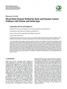
For the 2d-problems (## 58, 59, 64, 110) the initial nonmatching grids are given in Figure 1 and the initial mortar grids on all interfaces are given in Table 1. For 3d-problems (#104, #107) we consider similar (but 3d−) grids. We use α = 0.1.
Figure 1: Initial non-matching grids for Cases 1–3 mortar elements
1 3
2 3
3 1
4 5
Table 1: Initial number of elements in mortar grids for Cases 1–3
2.1 Case 1 The code was first modified to calculate the error over the interiors of all subdomains that have a one-element border around it. Tests were only run using mortar 4 (piecewise constant) because it was obvious that even there exist some improvement of the the rate of convergence of the interior error, it is not essential. The results for this case are in Table 2. The rates were established by running all tests for 5 levels of grid refinement (we halve the element diameters for each refinement) and computing a least squares fit to the error.
2.2 Case 2 The second modification of the code produced a scaled interior error. The calculation ||u − uh ||/||u|| over the interior subdomains was used in an attempt to eliminate any possible influence in the size of the interior subdomains would have on the error calculations. Again the improvement wasn’t essential. The results for this case are in Table 3.
3
test 58 59 64 104 107 110
velocity L2 error Cu αu 0.54367 0.78242 0.04109 0.52812 0.23754 1.15747 0.05610 0.47142 0.01157 1.78657 0.06674 0.57901
vel. L2 Cu 0.12750 0.01805 0.28418 0.02044 0.00073 0.01885
err. Int. αu 0.55476 0.62540 1.40638 0.51880 1.13243 0.57524
velocity L∞ error Cu αu 0.44620 0.26164 0.03793 0.04879 0.05094 0.19525 0.03826 -0.06980 0.01815 1.52227 0.05485 0.06251
vel. L∞ err. Int. Cu αu 0.21674 0.18728 0.01935 0.18330 0.10549 0.61198 0.02191 0.03434 0.00126 0.81571 0.08477 0.43350
Table 2: Velocity errors for Case 1 mortar 4
mor tar
1
2
3
4
test 58 59 64 104 107 110 58 59 64 104 107 110 58 59 64 104 107 110 58 59 64 104 107 110
velocity L2 error Cu αu 2.66274 1.77322 0.22929 1.69787 1.33161 1.78550 0.14553 1.55720 0.01688 1.95120 0.25459 1.46322 2.32761 1.71424 0.26758 1.81129 1.95992 1.96678 0.18661 1.61436 0.02004 2.00490 0.24784 1.45577 0.20265 0.70098 0.03542 0.75957 0.78962 1.65509 0.21352 1.00307 0.01509 1.91113 0.04343 0.75239 0.54367 0.78242 0.04109 0.52812 0.23754 1.15747 0.10682 0.48427 0.01157 1.78657 0.06674 0.57901
vel. L2 Cu 0.10485 0.28510 1.26313 0.03572 4.43731 0.12262 0.09601 0.28552 1.33080 0.05468 5.77645 0.11780 0.01260 0.05237 1.02173 0.09213 3.55414 0.01813 0.02276 0.04319 0.47748 0.03329 2.88170 0.02669
err. Int. αu 1.71342 1.92374 1.96919 1.65734 1.62768 1.81978 1.66598 1.93455 1.99125 1.76282 1.70399 1.80708 0.75098 1.12019 1.90811 1.19911 1.55203 0.94637 0.75181 0.82989 1.61093 0.61608 1.46652 0.77457
velocity L∞ error Cu αu 2.00771 1.24683 0.09980 0.94798 0.46868 0.86836 0.08844 0.88043 0.02860 1.72008 0.17738 0.96047 2.02304 1.24654 0.11920 1.20358 0.51878 1.25044 0.11574 0.96044 0.02962 1.72968 0.18424 0.96912 0.21370 0.21300 0.03058 0.24059 0.13897 0.74854 0.18577 0.38702 0.02489 1.66242 0.03563 0.25080 0.44620 0.26164 0.03793 0.04879 0.05094 0.19525 0.14464 -0.0051 0.01815 1.52227 0.05485 0.06251
Table 3: Velocity errors for Case 2
4
vel. L∞ err. Int. Cu αu 0.04331 1.34017 0.07066 1.31158 0.15226 1.34315 0.00888 0.83621 1.98867 1.17520 0.02718 1.08433 0.03760 1.29471 0.09820 1.44864 0.58127 1.86492 0.03387 1.17876 2.37342 1.22172 0.02429 1.06248 0.00286 0.17287 0.01960 0.51651 0.15094 1.39216 0.01875 0.30153 1.61587 1.12148 0.00494 0.21490 0.00897 0.31533 0.01400 0.21155 0.03592 0.76608 0.00842 -0.2289 0.92326 0.86969 0.00924 0.13240
2.3 Case 3 Thirdly, the code was modified to calculate the errors over fixed interior domains for each level of refinement. In this case it seems that the interior velocity error is superconvergent of O(h 2 ), which means that majority of the error occurs near the interfaces. Therefore we need to apply some local postprocessing to obtain better convergence rate for the velocity error. The results for this case are in Table 4 and Table 5. Plots of the computed solution and the numerical error for the case of mortar 4 are shown in Figure 2 through Figure 7. mor tar
1
2
3
4
test 58 59 64 104 107 110 58 59 64 104 107 110 58 59 64 104 107 110 58 59 64 104 107 110
flux error Cf αf 0.86618 1.14348 0.13611 1.02397 0.42816 0.99543 0.20796 1.34665 0.00634 1.51331 0.27076 1.30103 0.75732 1.06461 0.06147 0.96515 0.07839 1.00963 0.32708 1.41856 0.02873 2.03787 0.19697 1.19006 0.11513 0.12640 0.02008 0.08901 0.00923 0.22353 0.06591 0.19293 0.00238 1.24266 0.02073 0.05298 0.21224 0.11464 0.03114 -0.0819 0.02227 0.10901 0.06653 -0.1480 0.00107 0.81488 0.05203 -0.0242
pressure L2 error Cp αp 0.13977 2.00716 0.15428 1.99830 0.03591 2.00812 0.20782 2.02484 0.00132 2.01518 0.13936 2.00022 0.14012 2.00717 0.15483 1.99924 0.03109 1.95955 0.20910 2.02645 0.00152 2.05609 0.13997 2.00161 0.08315 1.79005 0.13470 1.96377 0.03283 1.98314 0.30498 1.93876 0.00127 2.00185 0.11937 1.94448 0.13560 1.77063 0.09478 1.76410 0.02811 1.78406 0.14887 1.53792 0.00127 1.98400 0.11900 1.78721
λ error Cλ αλ 0.25063 1.92904 0.18123 1.99922 0.07926 1.92863 0.10682 1.93479 0.00314 2.03247 0.12387 1.92116 0.24363 1.91795 0.16323 1.99847 0.08556 1.96633 0.15509 2.02785 0.00422 2.12012 0.14532 1.95482 0.73177 1.06345 0.06971 0.99552 0.02382 0.97858 0.06700 0.74369 0.00108 1.417078 0.08108 0.96348 0.12086 1.23240 0.07444 1.10489 0.01445 1.07005 0.13933 1.01947 0.00231 1.87368 0.08153 1.10277
Table 4: Velocity errors for Case 3 Part I
5
mor tar
1
2
3
4
test 58 59 64 104 107 110 58 59 64 104 107 110 58 59 64 104 107 110 58 59 64 104 107 110
velocity L2 error Cu αu 2.66274 1.77322 0.22929 1.69787 1.33161 1.78550 0.14553 1.55720 0.01688 1.95120 0.25459 1.46322 2.32761 1.71424 0.26758 1.81129 1.95992 1.96678 0.18661 1.61436 0.02004 2.00490 0.24784 1.45577 0.20265 0.70098 0.03542 0.75957 0.78962 1.65509 0.21352 1.00307 0.01509 1.91113 0.04343 0.75239 0.54367 0.78242 0.04109 0.52811 0.23754 1.15745 0.10682 0.48427 0.01157 1.78657 0.06674 0.57901
vel. L2 Cu 1.83728 0.20752 1.10879 0.08091 0.00615 0.17284 2.02425 0.20011 1.13106 0.13642 0.00796 0.17167 3.75547 0.32442 1.03225 0.78365 0.00503 0.25975 8.40882 0.42804 1.14140 0.42934 0.00446 0.54528
err. Int. αu 2.07849 2.01600 1.98649 1.96243 2.06281 1.97959 2.08969 2.00933 1.99507 2.10844 2.13705 1.97908 2.08824 2.03956 1.97148 2.04442 1.99090 2.03322 2.17624 1.99718 1.98235 1.63100 1.94802 2.04151
velocity L∞ error Cu αu 2.00771 1.24683 0.09980 0.94798 0.46867 0.86836 0.08844 0.88043 0.02860 1.72008 0.17738 0.96047 2.02304 1.24654 0.11920 1.20358 0.51878 1.25044 0.11574 0.96044 0.02962 1.72968 0.18424 0.96912 0.21370 0.21300 0.03058 0.24059 0.13897 0.74854 0.18577 0.38702 0.02489 1.66242 0.03563 0.25080 0.44620 0.26164 0.03793 0.04879 0.05094 0.19525 0.14464 -0.0051 0.01815 1.52227 0.05485 0.06251
Table 5: Velocity errors for Case 3 Part II
6
vel. L∞ err. Int. Cu αu 5.25444 1.90940 0.59001 1.97308 3.50649 1.97183 0.20929 1.77685 0.01078 1.74192 0.42815 1.89051 6.64471 1.94481 0.57503 1.96715 3.45547 1.96728 0.82962 2.14136 0.01424 1.81625 0.39475 1.87154 5.03022 1.66747 1.10888 1.98844 3.40828 1.96204 0.75907 1.47399 0.00767 1.61258 0.78292 1.97619 18.1699 1.86383 1.14213 1.87719 3.52201 1.97291 0.36614 0.97479 0.00687 1.59490 1.06262 1.82550
A. Computed pressure and velocity
B. Pressure and velocity error
Figure 2: Solution and error (magnified) for test#58 mortar4
A. Computed pressure and velocity
B. Pressure and velocity error
Figure 3: Solution and error (magnified) for test#59 mortar4
7
A. Computed pressure and velocity
B. Pressure and velocity error
Figure 4: Solution and error (magnified) for test#64 mortar4
A. Computed pressure and velocity
B. Pressure and velocity error
Figure 5: Solution and error (magnified) for test#104 mortar4
8
A. Computed pressure and velocity
B. Pressure and velocity error
Figure 6: Solution and error (magnified) for test#107 mortar4
A. Computed pressure and velocity
B. Pressure and velocity error
Figure 7: Solution and error (magnified) for test#110 mortar4
9
3 Error estimates in the case of discontinuous tensor Because it is hard to find problems with discontinuous tensor and known true solution for which the right-hand side f is a smooth function, we needed to make a bigger modification in the code. Thus, first the code was run for the finest grid and the solution was saved in files. Then the stored solution from this initial run was used to calculate the errors for all coarser grids. Again all examples are on the unit cube; the domain was divided into four equal subdomains. The initial grid in the case of matching grids was chosen to be 128×128. The initial nonmatching and mortar grids are shown in Table 6. 64 × 64 80 × 80
80 × 80 64 × 64
mortar elements
Non-matching grids
1 48
2 48
3 16
4 80
Mortar grids
Table 6: Initial grids for Case 4 In this case different test problems were tested. In problems 70 through 75 the permeability tensors were diagonal with piecewise constant diagonal elements. The prototype for the permeability tensor is
a(x, y) 0 0 0 a(x, y) 0 K= 0 0 a(x, y) where a(x, y) =
n 10
, if x < 1/2, y < 1/2
10n
, if x > 1/2, y > 1/2
1
, otherwise
For test problem#70,n = 1 and then n increments by 1 with each test problem through test#73. For test problem#74 2 , x < 1/2, y < 1/2 10 a(x, y) = 10 , x > 1/2, y > 1/2
For test problem#75
a(x, y) =
, otherwise
10
Test problem#170 is with full tensor
1
, x < 1/2, y < 1/2
102
, x > 1/2, y > 1/2
1
, otherwise
a(x, y) .1a(x, y) 0 K = .1a(x, y) a(x, y) 0 0 0 a(x, y)
where a(x, y) is as in test problem#70. The boundary conditions are Dirichlet on the left and right face and Neumann (no flow) on the rest of the boundary. For test problems#70,#71,#72, #73,#170 p|x=0 = 1 while for test problems#74 and #75 p|x=0 = 10
10
For all tests p|x=1 = 0
mortar 4
mortar 3
mortar 2
mortar 1
matching grids
The results for this case are in Table 7 and Table 8. Plots of the computed solution and the numerical error for test problems#71 and #170 are shown in Figure 8 and Figure 9. As the results show, because of the strong singularity at the cross-point (1/2, 1/2), there is no superconvergence even in the interior. The maximum rate of convergence for the interior velocity error is of O(h). Therefore to control the error we need some local refinement near this cross-point. Conclusion:Analyzing all test results in Section 2 and Section 3 we may conclude that interior velocity error depends on the smoothness of the solution in the whole domain Ω, but in more weak sense, and that interior velocity error is better than the velocity error calculated over the whole domain. test 70 71 72 73 74 75 170 70 71 72 73 74 75 170 70 71 72 73 74 75 170 70 71 72 73 74 75 170 70 71 72 73 74 75 170
flux error Cf αf 2.63071 0.14077 5.74425 0.09065 6.48755 0.07803 6.56845 0.07630 11.6789 0.12253 11.6788 0.12253 3.46109 0.28146 2.87058 0.14170 6.10402 0.09222 6.86057 0.07994 6.94565 0.07842 12.5847 0.12298 12.5850 0.12298 4.14805 0.28343 2.65103 0.11212 5.76999 0.06879 6.74202 0.07343 6.88443 0.07526 11.7169 0.09095 11.6919 0.09022 3.53285 0.20636 2.64355 0.10357 6.01293 0.08727 6.57508 0.07120 5.47429 -0.0072 11.7193 0.09411 11.7236 0.09421 3.52772 0.20854 2.81382 0.13225 6.06643 0.08742 6.83717 0.07650 6.92509 0.07519 12.4547 0.11595 12.4545 0.11595 3.98991 0.26285
pressure L2 error Cp αp 0.15364 1.05311 0.04845 0.67407 0.05149 1.03670 0.06634 1.11448 2.12416 0.91930 2.12416 0.91930 0.15389 1.05316 0.20148 1.06326 0.05755 0.67933 0.06501 1.03706 0.08507 1.11449 2.66909 0.92547 2.66909 0.92547 0.20179 1.06329 0.20343 1.18225 0.05757 0.67919 0.06499 1.03704 0.08507 1.11449 2.68899 0.92641 2.68410 0.92583 0.20374 1.06415 0.20035 1.05759 0.05943 0.70188 0.05660 1.11356 0.01310 0.54227 2.64884 0.92685 2.64983 0.92693 0.20067 1.05763 0.20157 1.07050 0.05798 0.68121 0.06511 1.03735 0.08508 1.11451 2.70630 0.93120 2.70630 0.93120 0.20186 1.07051
Table 7: Errors for Case 4 Part I
11
λ error Cλ αλ 0.77287 1.03731 0.25210 0.70538 0.03005 0.64297 0.00306 0.63601 8.95074 0.90491 8.95073 0.90491 0.77345 1.03728 1.00424 1.04344 0.30058 0.70927 0.03521 0.64615 0.00358 0.63884 11.2241 0.90994 11.2240 0.90994 1.00500 1.04342 0.99408 1.03561 0.27619 0.64336 0.03521 0.64616 0.00358 0.63921 11.1267 0.90294 11.1120 0.90253 0.99484 1.03559 0.30514 0.50878 0.10796 -0.0291 0.09621 -0.1143 0.41838 0.07096 3.72005 0.42120 3.71763 0.42069 0.30547 0.50888 1.03948 1.05073 0.30610 0.71235 0.03578 0.64901 0.00364 0.64196 11.5505 0.91556 11.5504 0.91556 1.04027 1.05071
matching grids mortar 1 mortar 2 mortar 3 mortar 4
test 70 71 72 73 74 75 170 70 71 72 73 74 75 170 70 71 72 73 74 75 170 70 71 72 73 74 75 170 70 71 72 73 74 75 170
velocity L2 error Cu αu 5.02826 0.80760 19.5352 0.60120 23.7806 0.55261 24.2655 0.54673 92.7638 0.73567 92.7634 0.73567 5.03173 0.80762 6.35111 0.80766 23.4454 0.60740 28.1822 0.55933 28.7154 0.55350 115.035 0.73837 115.030 0.73836 6.35561 0.80768 6.23825 0.79586 23.3687 0.60462 28.0979 0.55838 28.6897 0.55336 113.537 0.73029 113.523 0.73029 6.24275 0.79589 6.07333 0.79065 24.7832 0.63538 27.4119 0.56672 24.6847 0.49919 111.059 0.73119 111.091 0.73135 6.07766 0.79067 6.34711 0.80107 23.6418 0.60633 28.4218 0.55910 28.9680 0.55346 115.837 0.73468 111.091 0.73135 6.35174 0.80110
vel. L2 Cu 3.16430 9.33316 11.0525 11.2627 50.8235 50.8245 3.16635 20.5492 13.5818 15.8126 16.0688 77.4494 77.4548 4.98072 4.92724 13.5857 15.8298 16.0938 77.0655 77.0163 4.93047 20.2001 14.4814 15.1191 13.7162 76.1713 76.3615 4.89698 5.03046 13.7003 15.9559 16.2248 78.5609 76.3615 5.03374
err. Int. αu 1.13060 0.73624 0.66849 0.66136 0.96406 0.96407 1.13047 1.64331 0.73726 0.66910 0.66135 0.96422 0.96425 1.13034 1.12636 0.73701 0.66939 0.66192 0.96194 0.96173 1.12626 1.63663 0.76852 0.66777 0.58979 0.96367 0.96482 1.12373 1.13980 0.73942 0.67129 0.66390 0.97004 0.96482 1.13970
velocity L∞ error Cu αu 2.24790 -0.1318 9.49735 -0.2476 11.9794 -0.2722 12.2589 -0.2759 43.5174 -0.1777 43.5213 -0.1777 2.24876 -0.1318 2.86067 -0.1191 11.5272 -0.2309 14.4447 -0.2539 14.7786 -0.2572 54.3464 -0.1640 54.3452 -0.1640 2.86191 -0.1191 2.69003 -0.1528 10.9453 -0.2546 14.0227 -0.2649 14.4348 -0.2653 51.1419 -0.1942 51.1524 -0.1941 2.69127 -0.1528 2.89122 -0.1171 12.7548 -0.1867 14.8135 -0.2258 12.0942 -0.3260 55.0603 -0.1539 55.1061 -0.1537 2.89246 -0.1171 2.83992 -0.1323 11.6003 -0.2349 14.5522 -0.2560 14.8990 -0.2586 54.5911 -0.1724 54.5922 -0.1724 2.84132 -0.1323
Table 8: Errors for Case 4 Part II
12
vel. L∞ err. Int. Cu αu 7.24114 0.98681 22.2446 0.62329 26.6700 0.56086 27.2236 0.83473 123.086 0.83473 123.085 0.83473 7.24688 0.98681 22.0366 1.23625 28.8878 0.60806 33.5560 0.54250 34.1529 0.53564 172.361 0.82124 172.411 0.82136 10.6355 0.97250 10.0805 0.95716 28.4547 0.60378 33.4987 0.54209 34.0587 0.53482 166.450 0.81096 166.580 .81125 10.0881 0.95719 21.2636 1.22538 30.5703 0.63750 32.1567 0.54070 31.2366 0.47901 167.261 0.81792 167.482 0.81866 10.2909 0.96263 10.8196 0.98179 29.2555 0.61080 34.0070 0.54555 34.6187 0.53904 176.555 0.82858 176.507 0.82848 10.8275 0.98181
A. Computed pressure and velocity
B. Pressure and velocity error
Figure 8: Solution and error (magnified) for test#71 matching grids
A. Computed pressure and velocity
B. Pressure and velocity error
Figure 9: Solution and error (magnified) for test#170 matching grids
13
4 Influence of the low order term on the constant in the error estimates Theory indicates that the constant C in the error estimate ||p − ph || ≤ Ch2 depends on Kmax /Kmin . We study the dependence of the constant on the low order term α in (2). We tested three groups of problems. For all of them the permeability tensor K was chosen to be diagonal matrix with diagonal elements 1 2 a(x) = e−β(x− 2 ) where β is a real, nonnegative parameter. The values of β and corresponding values (approximately) of the ratio Kmax /Kmin are given in Table 9. β ratio
0 100
9 101
18.5 102
28 103
Table 9: Values of
37 104
46 105
Kmax Kmin
Test problems#81 and #82 used true analytic solutions. For test#81 p = 1 − x and for test#82 p = x3 y 4 + x2 + sin(xy) cos(y) For test#83 we used again files to save the solution for the finest grid. For this test f ≡ 0, p|x=0 = 1, p|x=1 = 0 and u · ν = 0 on ΓN .
ratio
For all test problems we used matching grids and the boundary conditions were Dirichlet on the left and right face and Neumann on the rest of the boundary. We compared the results when α = 0 (no low order term) and α = 1. The results are in Table 10 through Table 15.. Plots of the computed solution and the numerical error for α = 0 and α = 1 are shown in Figure 10 through Figure 15. They show that this method works very well for both cases even if there are big variations of K and that the constant increases very slowly when the ratio goes up.
100 101 102 103 104 105
α 0 1 0 1 0 1 0 1 0 1 0 1
flux error Cf αf 1.520E-05 -1.0184 2.520E-05 -0.8979 1.18544 1.00582 0.88688 1.01210 1.72450 1.00050 1.13756 1.02740 2.53682 1.00673 1.92024 1.04562 3.10393 1.01237 2.49763 1.04793 6.35081 2.03410 4.45480 2.09359
pressure L2 error Cp αp 5.223E-09 -0.4163 9.024E-09 -0.3304 1.11186 1.99857 1.05436 1.99651 2.55276 1.98550 2.16116 1.97790 4.54492 1.96592 2.87016 1.94721 6.74732 1.94627 3.31429 1.95384 9.10429 1.92649 3.74429 1.95838
Table 10: Errors for Test#81 Part I
14
λ error Cλ αλ 2.623E-08 -0.4938 4.684E-08 -0.3745 1.57440 1.99900 1.49051 1.99636 3.61007 1.98549 3.05399 1.97764 6.42815 1.96596 4.05745 1.94707 9.53957 1.94618 4.68600 1.95375 12.8703 5.29718 1.92635 1.95851
ratio 100 101 102 103 104 105
α 0 1 0 1 0 1 0 1 0 1 0 1
velocity L2 error Cu αu 1.959E-08 -0.8815 1.117E-08 -0.9970 0.91658 2.00282 1.04796 2.00076 1.60093 2.00913 1.87700 2.00235 2.06907 2.00956 2.37246 1.99846 2.51460 2.00756 2.79471 1.99700 2.83901 1.99846 3.11272 1.99131
vel. L2 err. Int. Cu αu 2.822E-08 -0.1845 3.896E-08 -0.1997 0.24832 1.97709 0.29905 1.97719 0.26881 1.93611 0.25119 1.91043 0.66296 2.00152 0.32107 1.99301 1.04688 2.03072 0.67433 2.11495 1.30681 2.03978 0.95971 2.12676
velocity L∞ error Cu αu 1.595E-08 -1.3747 2.907E-08 -1.2267 1.44057 1.94041 1.71072 1.95797 3.00145 1.96145 3.60231 1.96361 3.53206 1.93215 4.50453 1.93396 3.83614 1.89745 5.05376 1.90684 4.02057 1.86281 5.36164 1.87915
vel. L∞ err. Int. Cu αu 4.406E-08 -0.4704 9.665E-08 -0.3208 0.58024 1.85035 0.72373 1.86202 0.53670 1.81068 0.39762 1.65979 1.55599 1.95890 0.42730 1.73236 2.75755 2.00510 1.86876 2.06975 3.41880 2.00177 2.31484 2.04601
Table 11: Errors for Test#81 Part II
ratio 100 101 102 103 104 105
α 0 1 0 1 0 1 0 1 0 1 0 1
flux error Cf αf 0.48058 0.92198 0.39681 0.87120 1.58922 1.00151 1.31857 0.99968 2.16148 0.99954 1.55603 1.00823 3.12151 1.00590 2.36137 1.03718 3.81211 1.01168 3.05579 1.04467 9.61315 2.03300 6.68535 2.09079
pressure L2 error Cp αp 0.29886 1.99667 0.27677 1.99533 2.06764 1.99694 1.94081 1.99468 4.54800 1.98593 3.86108 1.97652 8.23068 1.96967 4.90257 1.94078 11.8719 1.94853 5.39610 1.94485 16.4131 1.76500 6.10213 1.95496
λ error Cλ αλ 0.39792 2.00045 0.37104 1.99594 2.85774 2.00007 2.64292 1.99813 6.26899 1.98799 5.28056 1.97920 12.5596 1.97820 6.93021 1.94673 17.8129 1.97492 7.68368 1.94838 23.0464 1.71409 8.61460 1.95559
Table 12: Errors for Test#82 Part I
ratio 100 101 102 103 104 105
α 0 1 0 1 0 1 0 1 0 1 0 1
velocity L2 error Cu αu 0.51967 1.98672 0.52388 1.97723 1.70894 1.99882 1.87290 1.99771 2.74123 2.00611 3.16910 2.00064 3.46317 2.00788 3.93653 1.99727 4.16972 2.00827 4.60159 1.99738 4.73005 2.00294 5.14499 1.99477
vel. L2 err. Int. Cu αu 0.18760 1.99842 0.19538 1.99463 0.68123 1.99665 0.71191 1.99283 0.69310 1.97321 0.71311 1.96552 1.12040 1.99457 0.69361 1.98080 1.64383 2.02131 1.05977 2.06600 2.02860 2.03314 1.45510 2.09869
velocity L∞ error Cu αu 1.32760 1.79569 1.27471 1.77775 4.27849 1.91655 4.47469 1.90753 9.01643 1.95499 10.2015 1.95629 11.7216 1.95136 13.7282 1.95030 13.4855 1.93658 15.9724 1.93683 14.9040 1.91828 17.6947 1.92183
Table 13: Errors for Test#82 Part II
15
vel. L∞ err. Int. Cu αu 0.90474 1.91797 0.91529 1.91845 2.55625 1.89986 2.84745 1.90317 1.59156 1.72722 2.62397 1.78597 2.96550 1.92528 1.57091 1.68975 5.16595 1.99412 2.13064 1.81785 6.82549 2.00437 4.56553 2.01597
flux error ratio 100 101 102 103 104 105
α 0 1 0 1 0 1 0 1 0 1 0 1
Cf 4.342E-06 3.803E-06 1.69532 1.28574 1.66590 0.56148 0.66009 0.75200 0.19089 0.88100 0.04673 0.74871
αf 0.38460 0.38418 2.08386 2.08814 2.08796 2.22665 2.10511 1.96891 2.13192 1.93894 2.16905 1.88571
pressure L2 error Cp αp 6.309E-08 0.33978 6.318E-08 0.35544 1.02830 2.06002 0.98923 2.06111 2.56514 2.00134 2.41972 2.01461 3.59111 1.92632 3.24561 1.97698 4.01591 1.85285 2.32435 1.92743 4.09979 1.78221 1.42642 1.80294
λ error Cλ αλ 3.564E-07 0.19340 3.321E-07 0.20265 1.45382 2.05990 1.39853 2.06099 3.62735 2.00131 3.42218 2.01463 5.07830 1.92629 4.58996 1.97698 5.67940 1.85285 3.28695 1.92741 5.79796 1.78221 2.01720 1.80293
Table 14: Errors for Test#83 Part I
ratio 100 101 102 103 104 105
α 0 1 0 1 0 1 0 1 0 1 0 1
velocity L2 error Cu αu 6.315E-07 -0.0915 6.366E-07 -0.0597 1.20316 2.08523 1.02448 2.09032 1.17719 2.08771 0.59393 2.13819 0.46627 2.10473 0.50664 1.96340 0.13499 2.13195 0.57140 1.93648 0.03302 2.16883 0.45583 1.87963
vel. L2 err. Int. Cu αu 8.596E-08 0.39917 1.033E-07 0.39344 0.60161 2.08525 0.47528 2.09072 0.58860 2.08771 0.19821 2.22732 0.23314 2.10473 0.28805 1.97335 0.06750 2.13195 0.31943 1.93825 0.01651 2.16883 0.23836 1.86526
velocity L∞ error Cu αu 5.106E-07 -0.7172 4.386E-07 -0.7236 1.08091 2.04545 1.15857 2.02808 1.13300 2.07356 0.71378 1.91463 0.45246 2.09366 0.62015 1.97963 0.13153 2.12240 0.71538 1.95218 0.03205 2.15785 0.61667 1.90274
vel. L∞ err. Int. Cu αu 2.225E-07 0.15937 3.156E-07 0.25133 1.20239 2.08498 0.95384 2.06170 1.17688 2.08757 0.35860 2.08571 0.46596 2.10447 0.61683 1.97954 0.13498 2.13192 0.70779 1.94979 0.03302 2.16882 0.60471 1.89878
Table 15: Errors for Test#83 Part II
A. Computed pressure and velocity
B. Pressure and velocity error
Figure 10: Solution and error (magnified) for test#81 α = 0 β = 46 matching grids 16
A. Computed pressure and velocity
B. Pressure and velocity error
Figure 11: Solution and error (magnified) for test#81 α = 1 β = 46 matching grids
A. Computed pressure and velocity
B. Pressure and velocity error
Figure 12: Solution and error (magnified) for test#82 α = 0 β = 46 matching grids
17
A. Computed pressure and velocity
B. Pressure and velocity error
Figure 13: Solution and error (magnified) for test#82 α = 1 β = 46 matching grids
A. Computed pressure and velocity
B. Pressure and velocity error
Figure 14: Solution and error (magnified) for test#83 α = 0 β = 46 matching grids
18
A. Computed pressure and velocity
B. Pressure and velocity error
Figure 15: Solution and error (magnified) for test#83 α = 1 β = 46 matching grids
References [1] T. A RBOGAST, L. C. C OWSAR , M. F. W HEELER , AND I. YOTOV, Mixed finite element methods on nonmatching multiblock grids, SIAM J. Numer. Anal., 37 (2000), pp. 1295–1315. [2] T. A RBOGAST, M. F. W HEELER , AND I. YOTOV, Mixed finite elements for elliptic problems with tensor coefficients as cell-centered finite differences, SIAM J. Numer. Anal., 34 (1997), pp. 828–852. [3] L C. C OWSAR AND M. F. W HEELER, Parallel domain decomposition method for mixed finite elements for elliptic partial differential equations, in Fourth International Symposium on Domain Decomposition Methods for Partial Differential Equations, SIAM, Philadelphia, 1991. [4] L C. C OWSAR , C A. S AN S OUCIE ,
AND
I YOTOV, Parcel v1.04 User Guide, May 1996.
[5] R. G LOWINSKI AND M. F. W HEELER, Domain decomposition and mixed finite element methods for elliptic problems, in First International Symposium on Domain Decomposition Methods for Partial Differential Equations, SIAM, Philadelphia, 1988, pp. 144–172. [6] I. YOTOV, Mixed finite element methods for flow in porous media, PhD Thesis, Rice University, Houston, Texas. TR96-09, Dept. Comp. Appl. Math., Rice University and TICAM report 96-23, University of Texas at Austin.
19