Proceedings of the ASME 2007 International Design Engineering Technical Conferences & Computers and Information in Engineering Conference IDETC/CIE 2007 September 4-7, 2007, Las Vegas, Nevada, USA
DETC2007-34754
COMPARISON OF THREE-DIMENSIONAL FLEXIBLE THIN PLATE ELEMENTS FOR MULTIBODY DYNAMIC ANALYSIS: FINITE ELEMENT FORMULATION AND ABSOLUTE NODAL COORDINATE FORMULATION
A. L. Schwab Laboratory for Engineering Mechanics Delft University of Technology Mekelweg 2, NL-2628 CD Delft The Netherlands Email:
[email protected]
J. P. Meijaard J. Gerstmayr School of MMME Institute of Technical Mechanics The University of Nottingham Johannes Kepler University of Linz University Park, Nottingham NG7 2RD Altenbergerstr. 69, A-4040 Linz United Kingdom Austria Email:
[email protected] Email:
[email protected]
ABSTRACT Three formulations for a flexible 3-D thin plate element for dynamic analysis within a multibody dynamics environment are compared: a classical Discrete Kirchhoff Triangle (DKT) with large displacements and large rotations, a fully parametrized rectangular element according to the absolute nodal coordinate formulation (ANCF) and a rectangular element according to the ANCF with an elastic midplane approach. The comparison is made by means of a small deformation static test and extensive eigenfrequency analyses on a stylized problem. It is shown that the DKT element can describe arbitrary rigid body motions and that both the DKT element and the thin plate ANCF element show good convergence to analytic solutions by increasing number of elements, and suppress shear locking which is present in the fully parametrized ANCF element.
reduce the number of degrees of freedom. A different way to describe the motion of the elements is by using nodal coordinates that describe the configuration of the element with respect to an inertial reference frame. This approach is more in line with traditional non-linear finite element formulations used in statics. A convenient element formulation was given by Van der Werff and Jonker [4], which was implemented in the program SPACAR [5] and extended further thereafter [6,7]. In this formulation, for each type of element a number of generalized deformations are defined that are invariant under rigid body motions, so arbitrary rigid body motions can exactly be described. More recently, another approach using nodal coordinates, the absolute nodal coordinate formulation (ANCF), was proposed by Shabana [8]. This finite element formulation describes the position of a material point within the element by interpolations based on the Cartesian absolute coordinates of the nodal points and on gradients of these positions with respect to a reference configuration. The use of gradients allows the exact representation of inertia parameters of a rigid body and avoids redundancy of rotational parameters for arbitrary large rotations. The resulting element mass matrix is constant, at the cost of a more complicated description for the stiffness. This allows an efficient formulation of the equations of motion for implicit time integration without repeated factorizations of element matrices [9]. The basic concept of so-called fully parametrized beam
1
Introduction The purpose of this paper is to make a comparison of some results obtained by two different formulations for describing the motion of three-dimensional flexible plates in a multibody dynamics context. A common approach found in the literature is to use a small displacement formulation with respect to a reference frame that describes the overall rigid-body motion of the plate [1] or to use a geometrically exact shell model [2, 3]. Including a limited set of assumed modes for the deformations can 1
c 2007 by ASME Copyright °
[10, 11] and plate [12] elements is using the position and three slope vectors as the nodal coordinates to interpolate the displacement field of the element. The three slope vectors form the components of the deformation gradient at a node which can represent arbitrary deformation states. However, the full parametrization leads to very high stiffness coefficients for the transverse normal deformations and cross-sectional distortion, which can cause ill-conditioned equations of motion, resulting in slow convergence and large simulation times [13]. The first paper to mention convergence problems in the ANCF has been presented by Sopanen and Mikkola [14]. They state that the convergence can be improved if the constitutive model is modified by setting the Poisson ratio to zero, however, they thought that the beam element would not suffer from shear locking. Later on, Gerstmayr and Shabana [15, 16] found coupled shear and thickness locking for the case of zero Poisson ratio, interpreted the locking effect as a result of the incompatible interpolation of bending and thickness deformation, and introduced alternative formulations in order to correct this effect. Independently, Schwab and Meijaard [17] came to the same conclusions and introduced an elastic line model for the absolute nodal coordinate beam element that relaxes the constraints for the cross-section deformation, eliminates shear locking by means of the Hellinger-Reissner principle and corrects shear and torsional stiffness by means of classical shear factors. Recently, Dmitrochenko and Pogorelov [18] developed an ANCF thin plate formulation which neglects the deformation of the cross-section and thus leads to a better computational performance with a reduced number of coordinates. Surprisingly, available contributions concerning the derivation of the fully parametrized ANCF plate element [12] and the thin plate element [13, 18], do not investigate the convergence properties for small plate thickness or locking effects.
2 SPACAR plate element The SPACAR plate element is a classical 3-D triangular thin plate element embedded in a multibody dynamics environment. Its characteristics are large displacements and large rotations but small, but finite, deformations. The element can be compared to a classical Discrete Kirchhoff Triangle (DKT) [21].
ez3
ey3
L3 = 1 r3
ex3 L1 = 0 ez2
L2 = 0 ez1
ey2
ey1 r2
z
r1 L1 = 1
ex1
h
ex2
L2 = 1
L3 = 0
y O
x
Figure 1. Three-dimensional triangular thin plate element with 3 nodes and 6 degrees of freedom in every node together with the triangular coordinates (L1 , L2 , L3 ).
The configuration of the element (see Figure 1) is determined by the position and orientation of the three nodes, by which it can be coupled to and interact with other elements. The positions of the nodes 1, 2, and 3 are given by their coordinates r1 , r2 , and r3 in a global inertial system Oxyz, whereas the orientations in the nodes are determined by orthogonal triads of unit vectors (ex1 , ey1 , ez1 ), (ex2 , ey2 , ez2 ), and (ex3 , ey3 , ez3 ) which are rigidly attached to the material in the direct vicinity of the nodes. The unit vector ez is perpendicular to the midplane of the plate and the unit vectors ex and ey are in-plane. In the absence of shear deformation, ex and ey are tangent to the elastic midplane of the plate. The change in orientation of the triads at the nodes is determined by an orthogonal rotation matrix R. This matrix can be parametrized by a choice of parameters, denoted by ϑ , such as Euler angles, Rodrigues parameters or Euler parameters. In the SPACAR software system [5], Euler parameters are used, but this choice is immaterial to the description of the element. For instance, the rotated unit z-vector in node 2 is given ϑ2 )e0z2 , where e0z2 is the unit vector in the initial unby ez2 = R(ϑ deformed configuration.
All three discussed plate elements are considered to be used in multibody system problems where large rigid body motions and small or large elastic vibrations need to be modelled. However, for the sake of comparison of the element formulation with each other and analytic solutions, small deformation static problems and eigenvalue analyses are used. The accuracy and convergence properties are assessed. All computations for the ANCF elements are performed with the flexible multibody code HOTINT [19, 20] and the eigenvalue problems are solved with MATLAB. The organization of the paper is as follows. After this introduction, a classical Discrete Kirchhoff Triangle with large displacements and large rotations is described and subsequently the ANCF fully parametrized and thin plate elements are described. Then results of a small deformation statics test and an extensive eigenfrequency analysis on stylized problems is presented and discussed. The paper ends with some conclusions. 2
c 2007 by ASME Copyright °
2.1
Elastic Forces The elastic forces are derived from the elastic midplane concept where transverse shear deformation is not taken into account, the so-called thin plate approach. The Kirchhoff-Love plate theory [22] is used. The element has 6 degrees of freedom as a rigid body, while the nodes have 3 × 6 = 18 degrees of freedom. Hence the deformation of the element determined by the position and orientation of the nodes can be described by 12 independent generalized strains. These strains are usually non-linear functions of the position and orientation of the nodes and the initial undeformed geometry. They can be compared to what Argyris [23] called natural modes, and will be invariant under arbitrary rigid body motions and thus truly measure the amount of strain in the element. The edges are identified by indices corresponding to nodes at the opposite vertex and then the edge vectors are given by l1 = r3 −r2 , l2 = r1 −r3 , and l3 = r2 −r1 . The length of the edges in the initial undeformed geometry are `1 , `2 , and `3 . Then the in-plane deformation can be described by the following 3 generalized strains, εi = (lTi li − `2i )/(2`i ),
i = 1, 2, 3,
a total of 10 coefficients is needed, which could be provided by the 3 transverse rigid body motions and 7 independent deformation modes. However, there are only 6 generalized transverse strains (2) and therefore an extra condition is needed to obtain a unique interpolation. This condition is the ability to describe constant curvature and a symmetry requirement [24]. The resulting transverse displacement field w¯ is then given by w¯ =
(3)
Indeed, taking directional derivatives of w¯ in the nodes along the edges results in the small angles corresponding to (2). The generalized stress–strain relations can be derived as follows. If we group the positions and orientations of the nodes in a vector x = (r1 , ϑ 1 , r2 , ϑ 2 , r3 , ϑ 3 ) and denote the vector of generalized deformations by ε , then we can write for the generalized strains (1) and (2) symbolically εi = Di (xk ),
(1)
i = 1, . . . , 9, k = 1, . . . , 18.
(4)
The dual quantities of the generalized strains ε are the generalized stresses σ . The physical meaning of these stresses is found by equating the internal virtual power of the elastic forces σ T δε˙ to the external virtual power fT δ˙x of the nodal forces. Substitution of the virtual generalized strains derived from (4) results in
which are the elongations of the edges to first order. This quadratic expression simplifies the description considerably with respect to expressions using the true change in length. This still leaves 3 in-plane degrees of freedom which we identify as the rotation of the triads in every node about the local z-axis (‘drilling’). Since these 3 are not sufficient to increase the order of the in-plane deformation in a uniform way (4 are needed), and no additional generalized strains are defined, this spurious motion without associated deformation will be constrained at each node. For the transverse bending deformation we define the following 6 generalized strains, ε4 = −eTz2 l1 , ε5 = eTz3 l1 , ε6 = −eTz3 l2 , ε7 = eTz1 l2 , ε8 = −eTz1 l3 , ε9 = eTz2 l3 .
ε4 (L22 L3 + L1 L2 L3 /2) + ε5 (L32 L2 + L1 L2 L3 /2) +ε6 (L32 L1 + L1 L2 L3 /2) + ε7 (L12 L3 + L1 L2 L3 /2) +ε8 (L12 L2 + L1 L2 L3 /2) + ε9 (L22 L1 + L1 L2 L3 /2).
σi δε˙ i = σi Di,k δx˙k = fk δx˙k
∀ δx˙k ,
(5)
where the Einstein summation convention over repeated indices is applied and a subscript after a comma denotes a partial derivative. From this we derive the equilibrium conditions for the element as fk = Di,k σi ,
(6)
Next we tie the generalized stresses σi to the generalized strains εi by the linearly elastic material behaviour. For the (x, ¯ y) ¯ in-plane behaviour we start from the plane stress–strain equations ε¯ x 1 −ν 0 σ¯ x 1 ε¯ y = −ν 1 σ¯ y 0 (7) E τ¯ xy γ¯ xy 0 0 2(1 + ν)
(2)
Here, eTzi l j can be identified as the approximate slope angle at node i of edge j times the length of edge j with respect to the initial plane configuration. The transverse displacement w¯ with respect to the plane through the three nodal points can be constructed. Instead of using the usual (x, ¯ y) ¯ in-plane coordinates, the description is simplified by using natural or triangular coordinates (L1 , L2 , L3 ), where each Li is zero along edge i and takes the values 1 at the opposite node i. Obviously, these coordinates, 0 ≤ Li ≤ 1 inside the triangle, fulfil the relation L1 + L2 + L3 = 1. For a full quadratic transverse displacement field w¯ in (L1 , L2 , L3 )
Here, E is the modulus of elasticity (Young’s modulus) and ν Poisson’s ratio. The generalized in-plane strains (1) can be expressed in terms of the physical strains ε¯ by the transformation εi = (ε¯ x cos2 φi + ε¯ y sin2 φi + γ¯ xy sin φi cos φi )li ,
i = 1, 2, 3, (8)
where φi is the angle of edge i with respect to the in-plane x3
c 2007 by ASME Copyright °
axis, considered positive for a rotation towards the y-axis. The generalized stresses correspond to uniaxial stresses in directions parallel to the sides of the triangle, σ¯ i = σi li /(Ah), where A is the in-plane area of the triangular plate element and h the transverse plate thickness. Transforming the physical strains and applying the dual transformation to the physical stresses results in the generalized stress–strain expressions εi = Fi j σ j with the inplane flexibility matrix Fi j =
1 `i ` j [(1 + ν) cos2i j −ν], EAh
i, j = 1, 2, 3,
the natural coordinate integral expressions Z A
with
Si j = (Fi j )−1 .
i, j = 4, . . . , 9,
where we used the transverse stiffness matrix 1ν 0 3 Eh ν 1 . 0 E¯ = 12(1 − ν2 ) 0 0 (1 − ν)/2
k = 1, . . . , 3,
j = 4, . . . , 9.
k, l = 1, . . . , 3, i, j = 4, . . . , 9.
(16)
i, j = 1, . . . , 9,
k = 1, . . . , 18,
(17)
where the coupling terms between the in-plane and transverse deformation, Smn and Snm for m = 1, . . . , 3 and n = 4, . . . , 9, are equal to zero. Finally, the element stiffness matrix is obtained by taking partial derivatives of the nodal elastic forces (17) with respect to the nodal coordinates x, resulting in a tangent stiffness matrix
(10)
K¯ kl = Di,k Si j D j,l + Di,kl σi ,
l = 1, . . . , 18.
(18)
The second part is the geometric stiffness matrix, which, evaluated in the undeformed and unstressed geometry, is equal to zero, whereas the first part is the linear stiffness matrix
(11)
Kkl = Di,k Si j D j,l .
(19)
The rank of this stiffness matrix is 9 and the three constraints on the rotation of a triad in every node about the z-axis have to be added.
(12)
2.2 Mass Matrix The derivation of the consistent mass matrix for the flexible thin plate element is based on the elastic midplane concept, where rotary inertia of the cross-section will be neglected. The cubic interpolation for the position of a point r = (xr , yr , zr ) on the elastic midplane in terms of triangular coordinates Li is taken as
(13)
T (L13 + 3L12 (L2 + L3 ) + 2L1 L2 L3 )I3 x1 (L12 L2 + L1 L2 L3 /2)I3 t13 2 (L L3 + L1 L2 L3 /2)I3 t12 13 (L + 3L2 (L3 + L1 ) + 2L1 L2 L3 )I3 x2 2 22 t21 = Nq, (20) r= (L2 L3 + L1 L2 L3 /2)I3 (L2 L1 + L1 L2 L3 /2)I3 t23 2 (L3 + 3L2 (L1 + L2 ) + 2L1 L2 L3 )I3 x3 3 3 (L2 L1 + L1 L2 L3 /2)I3 t32 3 2 t31 (L3 L2 + L1 L2 L3 /2)I3
the curvatures κ can be written as linear functions of generalized transverse strains εi as in κi = B i j ε j ,
Bki E¯kl Bl j dA,
fk = Di,k Si j ε j ,
The curvatures are derived in the usual manner from the transverse displacement w¯ (3) by κx = ∂2 w/∂ ¯ x¯2 , κy = ∂2 w/∂ ¯ y¯2 , and 2 κxy = ∂ w/∂ ¯ x∂ ¯ y. ¯ Again, natural coordinates Li will be used and with the help of the well-known transformation from natural coordinates to in-plane coordinates 1 1 1 1 L1 x¯ = x¯1 x¯2 x¯3 L2 , y¯ y¯1 y¯2 y¯3 L3
A
This, together with the in-plane stiffness matrix (10) gives the expressions for the nodal elastic forces
(9)
Z
¯ κdA = 1 εi Si j ε j , κ T Eκ 2 A
(15)
Z
Si j =
For the transverse stiffness we start from elastic bending energy expressed in terms of the curvatures κ = (κx , κy , 2κxy )T which we equate to the transverse bending energy expressed in terms of the generalized strains as in 1 Wb = 2
p!q!r! A, (p + q + r + 2)!
leads to the transverse stiffness matrix
with cosi j = lTi l j /(`i ` j ). By inverting the matrix Fi j we can write the in-plane generalized stresses in terms of the strains as σi = Si j ε j ,
p q
L1 L2 L3r dA = 2
(14)
The matrix Bi j holds constants from the initial geometry of the element and, with w¯ cubic, describes a curvature which is linear in Li over the element. Substitution of these curvatures in the transverse bending energy and integrating over the area, using 4
c 2007 by ASME Copyright °
where we have introduced the tangent vector ti j at node i along edge j. They are defined as t13 = a3 ex1 + b3 ey1 , t21 = a1 ex2 + b1 ey2 , t32 = a2 ex3 + b2 ey3 ,
t12 = −(a2 ex1 + b2 ey1 ) t23 = −(a3 ex2 + b3 ey2 ) t31 = −(a1 ex3 + b1 ey3 ),
r(4) ,z r(4)
elastic midplane z
(1) r(1) ,z r
h
(1)
r unit reference element
where we used the (x, ¯ y) ¯ in-plane dimensions a1 = x¯3 − x¯2 , a2 = x¯1 − x¯3 , a3 = x¯2 − x¯1 b1 = y¯3 − y¯2 , b2 = y¯1 − y¯3 , b3 = y¯2 − y¯1
Figure 2.
1 r˙ r˙ dA = x˙ T M˙x, 2 A
(23)
hi =
(25)
Z
CT NT NCdA = CT WC,
(2)
r
z
r,x(2)
y x
∂Mi j 1 ∂M jk − ∂xk 2 ∂xi
¶ x˙ j x˙k .
(28)
3 ANCF plate elements In the following, the mass and tangent stiffness matrices are derived for two large deformation plate elements based on the absolute nodal coordinate formulation. The first plate formulation concerns a fully parametrized (fp) 4-noded, rectangular, shear deformable plate element, where the position and three slopes are used as nodal degrees of freedom [12], see Figure 2. The second plate element is an improved formulation for 4-noded rectangular thin plates using only position and in-plane slopes as nodal coordinates. The strain energy depends on the deformation of the midplane only, not taking into account transverse shear effects, see Dmitrochenko and Pogorelov [18] and Dufva and Shabana [13]. The two elements have been implemented in the flexible multibody system code HOTINT [20]. Both formulations are derived at the same time, where the differences are marked with subindices fp and tp for the fully parametrized and the thin plate, respectively. For further details the referred papers should be consulted. The position vector of the plate in normalized element coordinates ξ ∈ [−1 . . . 1], η ∈ [−1 . . . 1], ζ ∈ [−1 . . . 1] is interpolated with shape functions S and nodal displacements,
Substitution of the above expressions in the kinetic energy integral leads to the mass matrix
A
,y
r,x(1)
r,x(3)
element in axis-parallel ref. configuration
µ
where the Ai and Bi matrices are the partial derivatives of the tangents ti j with respect to the angular parameters ϑ i and are given by
M = ρh
r
and every bold entry d stands for the matrix d ∗ I3 . This mass matrix is not constant, but depends on on the rotational parameters ϑ i via matrix C. Therefore, the inertia forces take on the form fin = −(M¨x + h), with the convective forces given by
where ρ is the volumetric mass density. Before evaluating the integral we need to express the time derivatives of the tangent vector ˙ti j in terms of time derivatives of the nodal coordinates x˙ as in C1 0 0 I3 0 q˙ = 0 C2 0 x˙ = C˙x, with Ci = 0 Ai , (24) 0 0 C3 0 Bi
ϑ1 , B1 = ∂t12 /∂ϑ ϑ1 , A1 = ∂t13 /∂ϑ ϑ2 , B2 = ∂t23 /∂ϑ ϑ2 , A2 = ∂t21 /∂ϑ ϑ3 , B3 = ∂t31 /∂ϑ ϑ3 . A3 = ∂t32 /∂ϑ
r(2) ,z r(2)
Nodal coordinates in the ANCF plate elements.
Z
T
(3)
(22)
In the initial geometry these tangents are simply plus or minus the corresponding edges. The mass matrix M is obtained from the kinetic energy integral 1 T = ρh 2
r(4)
,y
r,x(4)
,y
x
(21)
r(3) ,z r(3)
,y
(26)
where we introduced the mass coefficient matrix 1936 208 208 712 76 136 712 136 76 31 19 136 13 25 76 13 11 31 76 11 13 136 25 13 1936 208 208 712 76 136 ρhA 31 19 136 13 25 W= , 10080 31 76 11 13 1936 208 208 31 19 sym 31 (27)
rfp = Sfp (ξ, η, ζ)efp
and rtp = Stp (ξ, η)etp .
(29)
The shape functions are not unique for the 4-noded element; however, suitable third order interpolation functions with slope continuity at adjacent element edges are provided in the literature [12, 13]. The shape functions are incomplete up to cubic polynomials for the in-plane element coordinates ξ and η and linear with respect to the transverse coordinate ζ which is only used in the fully parametrized element. The nodal coordinates for a 5
c 2007 by ASME Copyright °
node i according to Figure 2 are given for the fully parametrized, h T (i) (i) efp = rfp
(i) T
rfp,x
(i) T
(i) T
rfp,y
rfp,z
iT
,
for a linear elastic material is given as WIfp =
(30)
and the thin plate element, h T (i) (i) etp = rtp
(i) T
(i) T
rtp,x
rtp,y
iT
T
e(2)
T
e(3)
T
e(4)
,
(31)
iT
.
(32)
£ ε m = Exx |ζ=0
∂x ∂ξξ
and xtp = Stp (ξ, η)e0tp ,
and
(33)
∂r ∂r = J−1 . ∂x ∂ξξ
ρST S|J| dV,
nT ∂2 r , ||n||3 ∂x2
1 WItp = 2
(34)
Eyy |ζ=0
2Exy |ζ=0
¤T
.
(38)
κyy =
nT ∂2 r ||n||3 ∂y2
and κxy =
Z ¡ ¢ εTm D2 εm + z2 κT D2 κ |Jtp | dV. V
(40)
Note that in the thin plate element, the element transformation Jtp only depends on the ξ and η coordinates. The integration over the volume is therefore performed for the ξ and η-coordinate in local element coordinates and for the z-coordinate over the thickness, −h/2 ≤ z ≤ h/2. The matrix of elastic material coefficients for the plane stress condition is given by
Z V
(37)
nT ∂2 r , ||n||3 ∂x∂y (39) where the normal to the deformed plate surface is defined as n = r,x × r,y . In the case of the thin plate element, the work of internal forces depends on the deformation of the element midplane (which leads to very similar in-plane deformation as in the fully parametrized element) and the bending deformation based on the curvatures, κxx =
The mass matrix is computed by integration of the density and the shape functions over the element volume, M=
ε T Dεε|J| dV,
The bending deformation of the plate is based on the curvatures κ = [κxx κyy 2κxy ]T which are defined by
where e0 is the vector of nodal coordinates in the undeformed reference configuration. The element transformation matrix J and the derivative with respect to global coordinates are given by J=
V
In the thin plate element, the work of internal forces is solely based on the deformation of the element midplane, ζ = 0, and thus only 3 components of the strain tensor are used that are evaluated at the midplane,
It should be noted that the formulation can be equally transformed to nodal displacements and displacement gradients, which is more common in finite elements but not considered in the original investigations of the ANCF. The derivative of the nodal coordinate r with respect to a coordinate α is defined by ∂r/∂α = r,α The relation of element coordinates ξ = [ξ η ζ]T and global coordinates x = [x y z]T is provided by the coordinate interpolation according to isoparametric elements xfp = Sfp (ξ, η, ζ)e0fp
Z
for the matrix of material coefficients D see the referred literature.
while the nodal coordinates of an element are denoted as h T e = e(1)
1 2
(35)
which gives a constant matrix. This is a specific feature of the ANCF which is usually not possible in large deformation structural elements.
1 E ν D2 = 1 − ν2 0
The virtual work of internal forces is based on the nonlinear Green strain tensor õ ¶ ! ∂r T ∂r 1 −I , (36) E= 2 ∂x ∂x
ν 0 1 0 0 (1 − ν)/2
(41)
For both elements, the tangent stiffness matrix is computed by means of twice differentiation with respect to the element coordinates e, µ ¶T ∂ ∂ WI . K= (42) ∂e ∂e
taking into account the element transformation Eq. (33) and the identity matrix I. In order to keep the notation simple, the engineering strains ε = [Exx Eyy Ezz 2Eyz 2Exz 2Exy ]T are used.
The first derivative of the work of internal forces is performed analytically and leads to the elastic forces, while the second derivative is computed by means of numerical differentiation in the program code HOTINT.
In the fully parametrized element, the work of internal forces 6
c 2007 by ASME Copyright °
ϕn = 0
3.1
Boundary conditions for the ANCF plate elements In the ANCF element, specific nodal coordinates need to be fixed in order to approximate the boundary conditions of the exact plate. The boundary conditions of the simply supported case with free rotation about the x-axis and free moving along the x-axis is approximated by fixing the nodal coordinates (i)
ry = 0,
(i)
rz = 0,
(i)
ry,x = 0 and
(i)
rz,x = 0,
F M
w=0 ϕn = 0
ϕn = 0 (a)
(43)
at each node i of the edge, compare Figure 2. The condition (i) r j,k = 0 means that the component j ∈ {x, y, z} of the derivative of the nodal position, ∂r/∂k, k ∈ {x, y, z}, is fixed. Alternatively, but not examined in the examples, one could think about fix(i) ing the component rx,y , meaning to enforce inplane y-fibers to be perpendicular to the axis of rotation at the boundary node. For the simply supported case, the same boundary conditions are used for the thin plate element and the shear deformable fully parametrized element. However, one could also constrain the (i) (i) plate normal components rx,z and ry,z , which is not performed in the examples. It turns out that for the present case of thin plates the influence of the alternative choice of constraints is negligible. The boundary conditions with respect to another axis of rotation follow by analogy to the above mentioned boundary conditions. For a boundary condition that represents the clamped case along an edge parallel to the x-axis, all nodal coordinates are fixed except the deformation perpendicular to the x-axis, which (i) (i) is ry,y and, for the fully parametrized plate, rz,z . Constraining (i) components such as ry,y at the boundary would mean to constrain the inplane deformation at the boundary which would result in (i) very slow convergence. The component rz,z could be constrained in principle for the fully parametrized element, but it does neither seem to be a realistic boundary condition nor would it lead to good convergence because of additional Poisson locking at the boundary. For the computation of inplane eigenmodes, the nodal coor(i) (i) (i) (i) dinates rz , rx,z and ry,z are fixed for the thin plate and rz,x and (i) rz,y are additionally fixed for the fully parametrized plate.
(b)
Figure 3. (a): Loading, boundary conditions and unform 4×4 meshing pattern of a square cantilevered plate with triangular elements. (b): Uniform doubly symmetric 4×4 meshing pattern of a square plate with triangular elements as used in dynamics tests.
the analytical exact solutions for the transverse displacement and normal rotation along the loaded edge are, wexact =
Ml 2 Fl 3 + , 2D 3D
and ϕexact =
Ml Fl 2 + , D 2D
(44)
where we used the elastic plate constant D = Eh3 /(12(1 − ν2 )). The test problem is modelled by a square plate with in-plane dimensions of l by l and a constant plate thickness h. For the ANCFfp element a value of h/l = 0.01 is used. The loading, boundary conditions, and uniform 4×4 meshing for the triangular element type are illustrated in figure 3.a. For the rectangular element types the same boundary conditions and uniform meshing grid but now without the diagonals is used. A Poisson ratio of ν = 0.3 has been used, unless otherwise stated. The static results for the three different element types are presented in Tables 1 and 2, where the displacements and rotations are normalized by the exact solutions according to (44). The two thin plate element formulations, SPACAR and ANCFtp, pass the static test. The ANCFtp is exact, whereas the convergence of the SPACAR results with refined mesh is good. Even the solutions for a 1×1 element mesh are already pretty accurate. The fully parametrized ANCF element shows Poisson locking, which was expected since the solution approaches the case for plane strain and the stiffness is too large by a factor of approximately (1 − ν)2 /(1 − 2ν). The second set of tests are eigenfrequency analyses on the free vibration of a thin square plate with three different sets of boundary conditions. The square plate has length l, thickness h and the material is isotropic linearly elastic with modulus of elasticity E, Poisson’s ratio ν and volumetric mass density ρ. The solutions depend on the value of Poisson’s ratio, and for all cases ν = 0.3 is used. The literature on the transverse vibration of plates is very rich. An in-depth survey on this subject was made in the 1970s by Leissa [25]. Some publications which are closely related to the test problem, a thin rectangular plate, will be discussed here. The first publication on this topic is the experimental work by
4
Results and Discussion To investigate the performance of the different element types a number of tests has been performed. The first test is a simple static test of a cantilevered plate under two loading conditions. The first loading case is a distributed moment along the free edge opposite the clamped edge. This should result in a constant bending moment in the plate. The second loading case is a distributed transverse force at this free edge. For an infinitely long plate of width l and constant thickness h (h/l ¿ 1) made out of isotropic homogenous linearly elastic material with modulus of elasticity E and Poisson ratio ν, 7
c 2007 by ASME Copyright °
Table 1. Average normalized transverse displacements w ¯ and rotations ϕ¯ for a square cantilevered plate loaded by a distributed moment at the
cies of rectangular plates. As a basis for comparison, we use ‘analytic’ results obtained by the Rayleigh-Ritz method with polynomial functions of the form xi y j as trial functions, as in [34], with the exponents i and j up to 15. The symmetry about axes parallel to the sides of the plate is used, but not the symmetry about the diagonals. The first case we consider here is the free transverse vibration of a completely free plate. Although somewhat idealized, this case has a number of advantages: there are no kinematic boundary conditions and it demonstrates the possibility of the element to describe the three transverse rigid bodies motions. The first ten dimensionless eigenfrequencies for an increasing number of elements are shown in three tables: Table 3 shows the results obtained with the SPACAR DKT element, Table 4 those with the ANCF thin plate element, Table 5 those with the ANCF fully parametrized element. The nodal lines, or contours of stationary points, for the first 32 vibration modes are drawn in Figure 4, the so-called Chladni figures. The three transverse rigid body motions are found within calculation precision for all three element types and are not mentioned in the tables. Both the SPACAR and the ANCF thin plate results converge rapidly, with increased mesh refinement, to the analytic results. The fully parametrized ANCF element slowly converges to values close to the analytic solutions. This is due to the Poisson locking; also the effect of shear locking can be seen in the high frequencies at a coarse mesh. For comparison, the results of the three elements with a 16×16 mesh are combined in Table 6. The results in literature do not always comply with the results as presented here. For instance Iguchi [29] reports a mode with frequency Ω = 6.62316 which is not found in the SPACAR nor in the ANCF analysis. Iguchi finds this mode in search of all modes which are symmetric with respect to the middle lines and antisymmetric with respect to the diagonals. Hence, the diagonals are always lines of nodes. For the first five of these modes Iguchi reports Ω = (1.98550, 6.62316, 11.86565, 16.36387, 29.75996), whereas the SPACAR analysis on a refined 20×20 mesh gives, by inspection of the Chladni figures for these modes (Figure 4), the following frequencies: Ω = (1.98168, 11.85936, 16.29010, 29.78484). The second case is the free transverse vibration of a completely simply supported (SSSS) square plate. The analytical results are straightforward and take the form of Ω = n2 + m2 where n and m are the number of half-wave modes in the x and y direction. For the finite element model the simply supported boundary conditions at the edges are imposed by setting all transverse displacements w to zero and all rotations normal the edges ϕn to zero. The first ten frequencies from an analysis with all three element types for a 16×16 mesh are shown in Table 7. The SPACAR DKT element and the ANCF thin plate element compare well with the analytical results. The fully parametrized ANCF element shows an offset of about 10%, which is due to the Poisson locking. Note that for (n, m) = (1, 3) and (n, m) = (3, 1)
free edge for a number of mesh refinements and three different element types: SPACAR, ANCF thin plate, and ANCF fully parametrized.
Mesh
1×1 2×2 4×4 8×8 16×16 1×1 2×2 4×4 8×8 16×16
SPACAR
ANCFtp
w¯ 1.021820 1.006890 1.002276 1.000799 1.000313 ϕ¯ 1.021328 1.012147 1.006495 1.003253 1.001605
w¯ 1.000000 1.000000 1.000000 1.000000 1.000000 ϕ¯ 1.000000 1.000000 1.000000 1.000000 1.000000
ANCFfp ν = 0.3 w¯ 0.816836 0.817157 0.818173 0.820056 0.823846 ϕ¯ 0.816634 0.816826 0.817485 0.818583 0.820741
ANCFfp ν = 0.0 w¯ 1.000360 1.000479 1.001113 1.002221 1.004478 ϕ¯ 1.000218 1.000221 1.000580 1.001123 1.002249
Table 2. Average normalized transverse displacements w ¯ and rotations ϕ¯ as in Table 1 but now loaded by a distributed transverse force at the free edge.
Mesh
1×1 2×2 4×4 8×8 16×16 1×1 2×2 4×4 8×8 16×16
SPACAR
ANCFtp
w¯ 1.026332 1.007233 1.002362 1.000844 1.000332 ϕ¯ 1.021820 1.006542 1.001975 1.000733 1.000303
w¯ 1.000000 1.000000 1.000000 1.000000 1.000000 ϕ¯ 1.000000 1.000000 1.000000 1.000000 1.000000
ANCFfp ν = 0.3 w¯ 0.612860 0.766434 0.806117 0.818371 0.826169 ϕ¯ 0.816788 0.817184 0.818214 0.820099 0.823887
ANCFfp ν = 0.0 w¯ 0.750425 0.938193 0.985977 0.999369 1.005687 ϕ¯ 1.000326 1.000479 1.001128 1.002238 1.004495
Chladni [26], who showed the vibration modes by means of the lines of nodes, now called Chladni figures. Then, around 1900, both Rayleigh [27] and Ritz [28] start calculating the modes and frequencies by means of assumed modes, the now called Rayleigh-Ritz method. One could say that in the work of Ritz lays the foundation of the Finite Element Method. After that a great many of people worked on the problem of which we mention here the following. Iguchi [29] shows eigenmodes and eigenfrequencies for a square plate, while Young [30] also includes other boundary conditions such as fully clamped. In a ¨ PhD thesis, Odman [31] calculates modes and frequencies for various boundary conditions and compares his results with those of others. Finally, Bartell et al. [32] and Gorman [33] are among the few that calculate the in-plane vibration modes and frequen8
c 2007 by ASME Copyright °
Table 3.
First ten dimensionless eigenfrequencies
Table 6.
Ω = ω/ω0 of the
No.
1×1 (12) 1.3087 2.1842 2.7075 4.1124 4.9627 8.0368 9.3307 11.3150 13.2777 –
1 2 3 4 5 6 7 8 9 10
2×2 (27) 1.3693 1.9657 2.4022 3.2989 3.5963 6.1316 6.7889 7.0339 8.1738 8.6570
4×4 (75) 1.3672 1.9893 2.4693 3.4782 3.5779 6.2010 6.2709 6.3842 7.1818 7.5753
8×8 (243) 1.3657 1.9873 2.4632 3.5142 3.5413 6.2011 6.2136 6.4265 7.0642 7.7709
16×16 Analytic (867) – 1.3647 1.3646 1.9860 1.9855 2.4602 2.4591 3.5226 3.5261 3.5298 3.5261 6.1937 6.1900 6.1961 6.1900 6.4454 6.4528 7.0294 7.0181 7.8076 7.8191
1×1 (36) 1.3895 2.2747 3.0998 4.1124 4.1124 9.1929 9.3307 9.3307 12.0850 –
1 2 3 4 5 6 7 8 9 10
Table 5.
2×2 (81) 1.3809 1.9819 2.4436 3.4167 3.4167 6.4302 7.0588 7.0588 7.6616 8.9273
4×4 (225) 1.3700 1.9922 2.4741 3.5158 3.5158 6.2594 6.2594 6.3489 7.0543 7.6272
8×8 (729) 1.3664 1.9876 2.4636 3.5251 3.5251 6.2138 6.2138 6.4188 7.0372 7.7839
No. 1 2 3 4 5 6 7 8 9 10
1 2 3 4 5 6 7 8 9 10
SPACAR (867) 1.364689 1.986028 2.460221 3.522614 3.529784 6.193704 6.196105 6.445354 7.029428 7.807619
ANCFtp (2601) 1.365120 1.986060 2.460272 3.526086 3.526086 6.196423 6.196423 6.444354 7.023856 7.811720
ANCFfp (3468) 1.373880 2.026803 2.786670 3.644811 3.644811 6.758548 6.812017 6.812017 7.292538 8.622965
Analytic 1.364614 1.985504 2.459086 3.526068 3.526068 6.190039 6.190039 6.452757 7.018053 7.819129
Table 7. First ten dimensionless eigenfrequencies Ω = ω/ω0 as in Table 6 but now for a completely simply supported (SSSS) plate.
16×16 Analytic (2601) – 1.3651 1.3646 1.9861 1.9855 2.4602 2.4591 3.5261 3.5261 3.5261 3.5261 6.1964 6.1900 6.1964 6.1900 6.4444 6.4528 7.0239 7.0181 7.8117 7.8191
No. 1 2 3 4 5 6 7 8 9 10
SPACAR (867) 1.989598 4.976733 4.976733 7.922142 9.905330 9.932462 12.811470 12.811470 16.905377 16.905377
ANCFtp (2601) 1.995853 4.983621 4.983621 7.935062 9.964255 9.964255 12.856629 12.856629 16.940498 16.940498
ANCFfp (3468) 2.219168 5.571218 5.571218 8.948634 11.224278 11.224278 14.650959 14.650959 19.279694 19.279694
Analytic 2 5 5 8 10 10 13 13 17 17
First ten dimensionless eigenfrequencies Ω = ω/ω0 as in Ta-
ble 3 but now modelled with rectangular ANCF fully parametrized plate elements. A relative plate thickness of h/l = 0.01 was used.
No.
Ω = ω/ω0 of the
in brackets are the number of degrees of freedom.
Table 4. First ten dimensionless eigenfrequencies Ω = ω/ω0 as in Table 3 but now modelled with rectangular ANCF thin plate elements.
No.
First ten dimensionless eigenfrequencies
free transverse vibration a completely free (FFFF) square plate with a 16×16 mesh and three different element types: SPACAR, ANCF thin plate, and ANCF fully parametrized together with the analytic results. For the ANCF fully parametrized a relative plate thickness h/l = 0.01 was used. The peigenfrequencies are nondimensionalized by the frequency ω0 = π2 D/(ρhl 4 ) and a Poisson ratio ν = 0.3 was used. Numbers
free transverse vibration a completely free (FFFF) square plate modelled by the SPACAR triangular elements for a number of mesh refinements. The peigenfrequencies are nondimensionalized by the frequency ω0 = π2 D/(ρhl 4 ) and a Poisson ratio ν = 0.3 was used. Numbers in brackets are the number of degrees of freedom.
1×1 (48) 1.4383 2.2738 3.5946 71.9937 71.9937 85.2672 93.5137 93.5144 93.7379 124.9953
Table 8. First ten dimensionless eigenfrequencies Ω = ω/ω0 as in Table 6 but now for a a completely clamped (CCCC) plate.
2×2 4×4 8×8 16×16 Analytic (108) (300) (972) (3468) – 1.4381 1.4245 1.3870 1.3739 1.3646 2.2737 2.0761 2.0396 2.0268 1.9855 3.5943 2.9252 2.8183 2.7867 2.4591 7.9943 5.5712 3.8033 3.6448 3.5261 7.9943 5.5712 3.8033 3.6448 3.5261 18.0359 7.8876 7.0251 6.7585 6.1900 18.0359 7.8876 7.0251 6.8120 6.1900 54.6686 14.9195 7.4395 6.8120 6.4528 72.2273 16.6870 7.9821 7.2925 7.0181 72.5239 17.6652 9.3389 8.6230 7.8191
No. 1 2 3 4 5 6 7 8 9 10 9
SPACAR (867) 3.624213 7.392791 7.392791 10.816637 13.215627 13.272338 16.412131 16.412131 21.205957 21.205957
ANCFtp (2601) 3.631785 7.397881 7.397881 10.833617 13.262707 13.331566 16.467135 16.467135 21.235469 21.235469
ANCFfp (3468) 4.088801 8.414502 8.414502 12.549341 15.271349 15.319996 19.387085 19.387085 24.775537 24.775537
Analytic 3.646062 7.436351 7.436351 10.964625 13.331920 13.395148 16.718040 16.718040 21.330322 21.330322
c 2007 by ASME Copyright °
Table 9.
1
=1.36462
2
=1.98168
3
=2.45254
4
=3.52292
No. 5
9
=3.52292
=7.01541
13
17
21
25
29
=11.85936
=15.41949
=20.11447
=21.67618
=29.22067
6
=6.19275
10
14
18
22
26
30
=7.81761
=12.39144
=16.29010
=20.72328
=24.51138
=29.78484
7
=6.19275
11
15
19
23
27
31
=10.66210
=13.31277
=16.98728
=21.65793
=24.51138
=30.04295
8
1 2 3 4 5 6 7 8 9 10
=6.44357
12
16
20
24
28
32
First ten dimensionless eigenfrequencies
Ω = ω/ωn of the
in-plane vibration a free (FFFF) square plate modelled by the SPACAR triangular elements for a number of mesh refinements together with the analytic results. pThe eigenfrequencies are nondimensionalized by the frequency ωn = E/(ρl 2 (1 − ν2 )). Numbers in brackets are the number of degrees of freedom.
=10.66210
=13.31277
1×1 (8) 2.5180 2.5548 2.9406 3.5083 4.9705 – – – – –
2×2 (18) 2.6219 2.7702 3.0959 3.0959 3.7230 4.0718 4.8375 4.8375 5.4041 6.3450
4×4 (50) 2.4751 2.6669 2.7938 2.7938 3.5635 3.6141 4.3794 4.3794 5.0060 6.1167
8×8 (162) 2.3709 2.5725 2.5725 2.6540 3.2023 3.4905 3.9905 3.9905 4.6859 5.4577
16×16 Analytic (578) – 2.3347 2.3206 2.4997 2.4716 2.4997 2.4716 2.6388 2.6284 3.0473 2.9874 3.4638 3.4522 3.8068 3.7231 3.8068 3.7231 4.4464 4.3031 5.1293 4.9686
=20.11447
tions for the SPACAR DKT element are straightforward, all degrees of freedom along the four edges are set to zero. Table 8 shows the first ten dimensionless eigenfrequencies as calculated with the three element types for a 16×16 mesh together with the analytical results. Again, these are in good agreement for the SPACAR DKT element and the ANCF thin plate element with the analytic results, and an offset for the fully parametrized ANCF element, due to Poisson locking. The frequency 5 and 6 ¨ are distinct and belong to different modes whereas Odman [31] reports equal frequencies. Young [30] does find a distinct frequency 6 and the mode resembles the SPACAR as well as the ANCF solutions closely.
=21.65793
=28.19405
=30.32299
Finally the in-plane vibration of a free (FFFF) square plate is considered. The results of the analysis with the SPACAR triangular element for increasing mesh refinements are presented in Table 9. There is a fairly good agreement. The SPACAR solution loses digits with increased frequency. This is probably due to low order of the element: the in-plane deformations are constant within one element. The corresponding eigenmodes are shown in Figure 5 and they compare well with the six modes presented by Bardell et al. [32]. The first eigenmode is a shear mode whereas the combination of the second and identical third eigenmode resemble a kind of in-plane bending mode. The results for all three element types for a 16×16 mesh are shown in Table 10. Both the ANCF thin plate element and the ANCF fully parametrized element give very accurate, nearly identical results. This is because of the higher order of interpolation, for one element the in-plane strains are interpolated up to second order opposed to constant for the SPACAR DKT element. This is also expressed in the number of degrees of freedom used.
Figure 4. First 32 transverse vibration modes together with their dimensionless frequencies Ω = ω/ω0 for a free (FFFF) square plate as calculated by the SPACAR triangular element with a mesh of 20×20. These are the so-called Chladni figures where the solid black lines within the square are the lines of nodes (contours of stationary points).
the analytical modes, with frequency 10, show up as distinct frequencies (i.e. 9.905330 and 9.932462) in the SPACAR analysis. The corresponding SPACAR modes have as lines of nodes respectively a diagonal cross and a centred circle. The centred circle can be constructed by a linear combination of the ”13” and ”31” mode, the diagonal cross can not. This is probably due to the meshing pattern. The third case for the free transverse vibration of a square plate is with all edges clamped (CCCC). The boundary condi10
c 2007 by ASME Copyright °
Table 10.
First ten dimensionless eigenfrequencies
Ω = ω/ωn of the
in-plane vibration a free (FFFF) square plate with a 16×16 mesh and three different element types: SPACAR, ANCF thin plate, and ANCF fully parametrized together with the analytic result. For the ANCF fully parametrized a relative plate thickness h/l = 0.01 was used. The p eigenfrequencies are nondimensionalized by the frequency ωn =
Ω1=2.32974
Ω2=2.48995
Ω3=2.48995
E/(ρl 2 (1 − ν2 )) and a Poisson ratio ν = 0.3 was used. Numbers in brackets are the number of degrees of freedom. No. 1 2 3 4 5 6 7 8 9 10
SPACAR (578) 2.334659 2.499734 2.499734 2.638791 3.047349 3.463758 3.806820 3.806820 4.446408 5.129318
ANCFtp (1734) 2.320595 2.471608 2.471625 2.628441 2.987382 3.452238 3.723111 3.723116 4.303086 4.968649
ANCFfp (2023) 2.320599 2.471620 2.471630 2.628445 2.987398 3.452212 3.723124 3.723124 4.303137 4.968699
Analytic 2.320597 2.471618 2.471618 2.628445 2.987385 3.452242 3.723115 3.723115 4.303079 4.968626
Ω4=2.63560
Ω =3.77860 7
Ω =3.02635 5
Ω8=3.77860
Ω6=3.45986
Ω =4.40102 9
Ω10=5.07746
5
Conclusion The comparison between the three types of plate element formulations, the discrete Kirchhoff triangle (DKT) developed for SPACAR, a rectangular element according to the fully parametrized absolute nodal coordinate formulation (ANCFfp) and the thin plate version of the latter (ANCFtp), shows their convergence characteristics and accuracy for small displacement problems. For in-plane problems, all elements show satisfactory results, where the convergence rate of the DKT is the least, which is due to its linear approximation of the displacements. For outof-plane problems, the DKT and ANCFtp elements show good accuracy and convergence, where the ANCFtp element gives a larger rate of convergence, which can be attributed to its ability to describe a full cubic displacement field. The ANCFfp element, however, suffers from locking and shows a very low rate of convergence, or no convergence at all, for thin plates in the general case. The locking can be of the Poisson type, where the contraction in the normal direction is hindered, or of the shear type, where transverse shear and bending are coupled.
Figure 5. First 10 in-plane eigenmodes together with their dimensionless frequencies Ω = ω/ωn for a free (FFFF) square plate as calculated by the SPACAR triangular element with a mesh of 16×16.
[2]
[3]
[4]
[5] Acknowledgements Support of J. Gerstmayr by an APART (Austrian Programme for Advanced Research and Technology) scholarship of the Aus¨ trian Academy of Sciences (OAW) is gratefully acknowledged.
[6]
REFERENCES [1] Neto, M. A., Ambr´osio, J. A. C., and Leal, R. P., ‘Composite materials in flexible multibody systems’, Computer 11
Methods in Applied Mechanics and Engineering 195, 2006, pp. 6860–6873. Simo, J. C. and Fox, D. D., ‘On a stress resultant geometrically exact shell model. Part I: Formulation and optimal parameterization’, Computer Methods in Applied Mechanics and Engineering 72, 1989, pp. 267–304. Bauchau, O. A., Choi, J.-Y., and Bottasso, C. L., ‘On the modeling of shells in multibody dynamics,’ Multibody System Dynamics 8(4), 2002, pp. 459–489. Werff, K. van der, and Jonker, J. B., ‘Dynamics of flexible mechanisms’, in Computer aided analysis and optimization of mechanical system dynamics, Haug, E. J. (ed.), SpringerVerlag, Berlin, 1984, pp. 381–400. Jonker, J. B., and Meijaard, J. P., ‘SPACAR–Computer program for dynamic analysis of flexible spatial mechanisms and manipulators’, in Multibody Systems Handbook, Schiehlen, W. O. (ed.), Springer-Verlag, Berlin, 1990, pp. 123–143. Meijaard, J. P., ‘Some developments in the finite element modelling and solution techniques for flexible multibody dynamical systems’, in Euroconference on Computational Mechanics and Engineering Practice, September 19–21, Szczyrk, Poland, conference Proceedings, Stadnicki, J. (ed.), University of Ł´od´z, branch in Bielsko-Biała, Bielskoc 2007 by ASME Copyright °
Biała, 2001, pp. 48–55. [7] Schwab, A. L., Dynamics of flexible multibody systems, small vibrations superimposed on a general rigid body motion, Ph.D. thesis, Delft University of Technology, Delft, 2002. [8] Shabana, A. A., ‘Definition of the slopes and the finite element absolute nodal coordinate formulation’, Multibody System Dynamics 1, 1997, pp. 339–348. [9] Gerstmayr, J. and Sch¨oberl, J., ‘A 3D finite element method for flexible multibody systems’, Multibody System Dynamics 15, 2006, pp. 309–324. [10] Shabana, A. A., and Yakoub, R. Y., ’Three dimensional absolute nodal coordinate formulation for beam elements: theory’, ASME Journal of Mechanical Design 123, 2001, pp. 606–613. [11] Yakoub, R.Y., and Shabana, A.A., ’ Three dimensional absolute nodal coordinate formulation for beam elements: implementation and applications’, ASME Journal of Mechanical Design 123, 2001, pp. 614–621. [12] Mikkola, A. M., and Shabana, A. A., ‘A non-incremental finite element procedure for the analysis of large deformation of plates and shells in mechanical system applications’, Multibody System Dynamics 9, 2003, pp. 283–309. [13] Dufva, K., and Shabana, A. A., ‘Analysis of thin plate structures using the absolute nodal coordinate formulation’, Proc. IMechE part K: Journal of Multi-body Dynamics 219, 2005, pp. 345–355. [14] Sopanen, J. T., ans Mikkola, A. M., ‘Description of Elastic Forces in Absolute Nodal Coordinate Formulation’, Nonlinear Dynamics 34, 2003, pp. 53–74. [15] Gerstmayr, J., and Shabana, A. A., ‘Efficient integration of the elastic forces and thin three-dimensional beam elements in the absolute nodal coordinate formulation’, in Multibody Dynamics 2005 - ECCOMAS Thematic Conference, Madrid, Spain, conference proceedings, Goicolea, Cuadrado, Garca Orden (eds.), 2005 (CDROM). [16] Gerstmayr, J., and Shabana, A. A., ’Analysis of thin beams and cables using the absolute nodal coordinate formulation’, Journal of Nonlinear Dynamics 45, 2006, pp. 109– 130. [17] Schwab, A. L., and Meijaard, J. P., ‘Comparison of threedimensional flexible beam elements for dynamic analysis: finite element method and absolute nodal coordinate formulation’, in Proceedings of IDETC/CIE 2005 ASME International Design Engineering Technical Conferences, Long Beach, CA, Paper Number DETC2005-85104, ASME, New York, 2005 (CDROM). [18] Dmitrochenko, O. N., and Pogorelov, D. Yu., ‘Generalization of plate finite elements for absolute nodal coordinate formulation’, Multibody System Dynamics 10, 2003, pp. 17–43. [19] Gerstmayr, J., and Stangl, M., ‘High-order implicit Runge-
[20] [21]
[22] [23]
[24] [25] [26] [27] [28]
[29]
[30]
[31] [32]
[33]
[34]
12
Kutta methods for discontinuous mechatronical systems,’ In Proceedings of XXXII Summer School APM, St. Petersburg, Russia, 2004. http://tmech.mechatronik.uni-linz.ac.at/ staff/gerstmayr/hotint.html Batoz, J. L., Bathe, K. J., and Ho, L. W., ‘A study of three-node triangular plate bending elements’, International Journal for Numerical Methods in Engineering 15, 1980, pp. 1771–1812. Timoshenko, S. and Woinowsky-Krieger, S., Theory of Plates and Shells, 2nd ed., McGraw–Hill, New York, 1959. Argyris, J. H., ‘Continua and discontunia, an aperc¸u of recent developments of the matrix displacement methods’, in Matrix Methods in Structural Mechanics, J. S. Przemienniecki, et al. (eds.), Wright-Patterson Air Force Base, Dayton, Ohio, 1966, pp. 11–189. Zienkiewicz, O. C., The Finite Element Method, McGrawHill, London, 3rd ed.[Ch. 10.6], 1977. Leissa, A. W., Vibration of Plates, NASA SP-160, Washington, DC, 1969. Chladni, E. F. F., Die Akustik, Breitkopf und H¨artel, Leipzig, 1802. Rayleigh, J. W. S., The Theory of Sound, Vol. I, 2nd ed., 1894. Ritz, W., ’Theorie der Transversalschwingungen einer Quadratischen Platte mit Freien R¨andern’, Annalen der Physik (4) 28, 1909, pp. 737–786. Iguchi, S., ‘Die Eigenschwingungen und Klangfiguren der vierseitig freien rechteckigen Platte’, Ingenieur-Archiv, 21, 1953, pp. 303–322. Young, D., ‘Vibration of rectangular plates by the Ritz method’, Journal of Applied Mechanics 17(4), 1950, pp. 448–453. ¨ Odman, S. T. A., Studies of boundary value problems, Ph.D. thesis, G¨oteborg, Sweden, 1955. Bardell, N. S., Langley, R. S., and Dunsdon, J. M., ‘On the free in-plane vibration of isotropic rectangular plates’, Journal of Sound and Vibration 191, 1996, pp. 459–467. Gorman, D. J., ‘Free in-plane vibration analysis of rectangular plates by the method of superposition’, Journal of Sound and Vibration 272, 2004, pp. 831–851. Kobayashi, Y., Yamada, G., and Honma, S., ‘In-plane vibration of point-supported rectangular plates’, Journal of Sound and Vibration 126, 1988, pp. 545–549.
c 2007 by ASME Copyright °