Finite Element Method of High-Order Accuracy for Solving Two

RUDN Journal of MIPh Вестник РУДН. Серия МИФ

2018 Vol. 26 No. 3 226–243 http://journals.rudn.ru/miph

UDC 519.632.4 DOI: 10.22363/2312-9735-2018-26-3-226-243

Finite Element Method of High-Order Accuracy for Solving Two Dimensional Elliptic Boundary-Value Problems of Two and Three Identical Atoms in a Line A. A. Gusev Laboratory of Information Technologies Joint Institute for Nuclear Research 6, Joliot-Curie str., Dubna, Moscow region, Russia, 141980 We considered models of three identical atoms in a line with molecular pair interactions and diatomic molecule scattered by an atom or tunneling through potential barriers. The models are formulated as 2D elliptic boundary-value problems (BVPs) in the Jacobi and polar coordinates. The BVP in Jacobi coordinates solved by finite element method of high-order accuracy for discrete spectrums of models under consideration. To solve the scattering problems the BVP in polar coordinates are reduced by means of Kantorovich method to a system of second-order ordinary differential equations with respect to the radial variable using the expansion of the desired solutions in the set of angular basis functions that depend on the radial variable as a parameter. The efficiency of the elaborated method, algorithms and programs is demonstrated by benchmark calculations of the resonance scattering, metastable and bound states of the considered models and also by a comparison of results for bound states of the three atomic system in the framework of direct solving the BVP by FEM and Kantorovich reduction. Key words and phrases: Elliptic Boundary-Value Problems, scattering problem, metastable and bound states, Kantorovich method

1.

Introduction

With the development of modern computing power, there are more possibilities for setting and numerically solving multidimensional boundary-value problems with high accuracy. For this, new numerical methods of high accuracy order are being developed. When reducing the boundary value problem to an algebraic one in the finite element method (FEM) of order 𝑝, one of the problems is the calculation of integrals on a finite element (we consider only simplicial finite elements) containing the products of two basis functions of Lagrange or Hermite interpolation polynomials of order 𝑝 by the coefficients for the unknown functions [1–3]. The FEM schemes and algorithms for solving the d-dimensional BVP are presented in [4–6]. The algorithms for constructing 2-dimensional fully symmetric Gaussian quadratures are presented in [7] while d-dimensional ones will be published elsewhere. The aim of this paper is to demonstrate the efficiency of the elaborated algorithms and program complexes KANTBP 4M, KANTBP 3, ODPEVP [8–10] by benchmark calculations of the resonance scattering below the dissociation threshold, metastable and bound states of the considered models and also by a comparison of results for bound states of the three atomic system in the framework of direct solving BVP by 2D FEM [3,7] and Kantorovich method (KM). We elaborated also algorithms for calculating the asymptotic parametric angular functions, the effective potentials and the fundamental solutions of the SODEs in the form of expansions by inverse powers of radial variable [11] and apply them to the construction of the asymptotic states of the triatomic scattering problem, because in three-atomic systems at large values of the hyperradial variable the effective potentials of SODEs have Received 27th May, 2018. The author thank Profs. O. Chuluunbaatar, V. L. Derbov, V. P. Gerdt, S. I. Vinitsky and Dr. L. L. Hai for collaboration. The work was supported by the RFBR (grants No. 16-01-00080 and 18-51-18005).

Gusev A. A. Finite Element Method of High-Order Accuracy for Solving . . .

227

the form of expansions in inverse powers of hyperradius even for short-range potentials of pair interactions. The paper is organized as follows. In Section 2 we formulate the 2D BVP for the dimer and trimer models. In Section 3 the 2D BVP in polar coordinates is reduced to the SODEs. In Sections 4, 5 and 6 we demonstrate the efficiency of the elaborated technique by test calculations of the resonance scattering of a diatomic molecule on an atom, the metastable and bound states of three atomic system, and the resonance tunneling of a diatomic molecule through a Gaussian barrier and the metastable states, respectively. In Conclusion the results and perspectives are discussed.

2.

Setting of the Problem

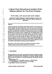
Consider a model of three identical particles (trimer) on a straight line with the masses 𝑀𝑖 = 𝑀 and the coordinates 𝑥 ¯𝑖 ∈ R1 , 𝑖 = 1, 2, 3, of one-dimensional Euclidian space 1 R coupled via the pair short-range potential 𝑉˜ (|¯ 𝑥𝑖 − 𝑥 ¯𝑗 |), 𝑖, 𝑗 = 1, 2, 3. Performing the change of variables corresponding to the cyclic permutation (𝛼, 𝛽, 𝛾) = (1, 2, 3) of the permutation group 𝑆3 [12]: √ 2 𝑥 ¯𝛼 + 𝑥 ¯𝛽 − 2¯ 𝑥𝛾 √ , 𝑥0 = √ (¯ 𝑥1 + 𝑥 ¯2 + 𝑥 ¯3 ), 𝑥𝛾 ≡ 𝑥(𝛼𝛽) = 𝑥 ¯𝛽 − 𝑥 ¯𝛼 , 𝑦𝛾 ≡ 𝑦(𝛼𝛽)𝛾 = 3 3 (︀ )︀𝑇 we get three pairs 𝑥(𝛼𝛽) , 𝑦(𝛼𝛽)𝛾 of the scaled Jacobi variables. In the center-of-mass reference frame of the configuration space x ¯ = (¯ 𝑥1 , 𝑥 ¯2 , 𝑥 ¯3 ) ∈ ℛ3 , i.e., on the hyperplane 3 Ω = {¯ x = (¯ 𝑥1 , 𝑥 ¯2 , 𝑥 ¯3 ) |¯ 𝑥1 + 𝑥 ¯2 + 𝑥 ¯3 = 0} ⊂ ℛ these Jacobi maps (𝑥, 𝑦)𝑇 ∈ Ω𝑥𝑦 ∼ ℛ2 are connected by the relations: (︂ )︂ (︂ )︂ (︂ )︂ 𝑥(𝛼𝛽) 𝑥𝛼 𝑥𝛾 ≡ = T𝑥𝑦 (𝜙𝛾𝛼 ) , 𝑦(𝛼𝛽)𝛾 𝑦𝛾 𝑦𝛼 (︂ )︂ (1) cos 𝜙𝛾𝛼 sin 𝜙𝛾𝛼 T𝑥𝑦 (𝜙𝛾𝛼 ) = , − sin 𝜙𝛾𝛼 cos 𝜙𝛾𝛼 where the angles 𝜙𝛾𝛼 = 𝜙𝛼𝛽 = 𝜙𝛽𝛾 = −𝜙𝛼𝛾 = −𝜙𝛽𝛼 = −𝜙𝛾𝛽 √ = (2𝜋)/3, i.e. cos 𝜙𝛾𝛼 = cos 𝜙𝛼𝛽 = cos 𝜙𝛽𝛾 = −1/2, sin 𝜙𝛾𝛼 = sin 𝜙𝛼𝛽 = sin 𝜙𝛽𝛾 = 3/2, are such that 𝜙𝛾𝛼 + 𝜙𝛼𝛽 + 𝜙𝛽𝛾 = 2𝜋, 𝜙𝛼𝛾 + 𝜙𝛽𝛼 + 𝜙𝛾𝛽 = −2𝜋. With the variable parameter 𝜙 in T𝑥𝑦 (𝜙) they and simply change the sign of pairs of Jacobi coordinates in Eq. (1), (︂ )︂ (︂ )︂ −𝑥(𝛼𝛽) 𝑥(𝛽𝛾) = T𝑥𝑦 (𝜙𝛾𝛼 ± 𝜋) . (2) −𝑦(𝛼𝛽)𝛾 𝑦(𝛽𝛾)𝛼 In Fig. 1 (a) the hyperplane (𝑥, 𝑦)𝑇 ∈ Ω𝑥𝑦 is separated by three axes 𝑦(12)3 , 𝑦(31)2 and 𝑦(23)1 into six sectors that together with three orthogonal axes 𝑥12 , 𝑥31 , 𝑥23 describe six channels of the scattering problem for three identical particles. Our choice is determined by the parameterization of the pairs (𝑦, 𝑥)𝑇 = (𝜌 cos 𝜙, 𝜌 sin 𝜙)𝑇 , where the angle 𝜙 ∈ [0, 2𝜋) is counted counterclockwise from the axis 𝑦(12)3 , for which 𝜙 = 0. As a result, we arrive at the Schr¨odinger equation for the wave function Ψ(𝑦, 𝑥) corresponding to the total energy 𝐸 of the triatomic system in Jacobi coordinates (𝑥, 𝑦)𝑇 = (𝑥𝛾 , 𝑦𝛾 )𝑇 ∈ Ω𝑥𝑦 : )︂ (︂ 𝜕2 𝑀 𝜕2 ˜ Ψ(𝑦, 𝑥) = 0. − 2 − 2 + 2 (𝑉˜ (𝑥, 𝑦) − 𝐸) (3) 𝜕𝑦 𝜕𝑥 ~

228

RUDN Journal of MIPh. Vol. 26, No 3, 2018. Pp. 226–243

✭❛✮

✭❜✮

Figure 1. (a) The profiles of 2D potential functions of Be3 in Jacobi coordinates (1) in the center-of-mass plane and the relative arrangement of particles in accordance with the region of the center-of-mass plane. The numbers of sectors are given in boxes. (b) The profiles of 2D potential functions of Be2 with barrier and the relative arrangement of particles and barrier. Here coordinates and potential functions are given in ˚ A and ˚ A−2 , respectively

In the case of a diatomic molecule (dimer) with identical nuclei coupled via the pair potential, 𝑉˜ (|¯ 𝑥1 − 𝑥 ¯2 |), moving in the external potential field 𝑉˜ 𝑏 (|¯ 𝑥𝑖 − 𝑥 ¯3 |), 𝑖 = 2, 1, of the third atom having the infinite mass, the same equation (3) is valid for the variables 𝑥 ≡ 𝑥3 = 𝑥 ¯2 − 𝑥 ¯1 ,

𝑦 ≡ 𝑦3 = 𝑥 ¯1 + 𝑥 ¯2 ,

with respect to the origin of the coordinate frame placed at the infinite-mass atom, 𝑥 ¯3 = 0. Here the potential function for the trimer with the pair potentials (below this case is referred to as Task 2, for example, see Fig. 1 (a)), ⃒)︃ ⃒)︃ (︃⃒ (︃⃒ ⃒ 𝑥 − √3𝑦 ⃒ ⃒ 𝑥 + √3𝑦 ⃒ ⃒ ⃒ ⃒ ⃒ 𝑉˜ (𝑥, 𝑦) = 𝑉˜ (|𝑥|) + 𝑉˜ ⃒ (4) ⃒ + 𝑉˜ ⃒ ⃒ , ⃒ ⃒ ⃒ ⃒ 2 2 or the potential function for a dimer in the field of a barrier potential (below this case is referred to as Task 3, see Fig. 1 (b)) ⃒)︂ ⃒)︂ (︂⃒ (︂⃒ ⃒𝑥 − 𝑦 ⃒ ⃒𝑥 + 𝑦 ⃒ 𝑏 𝑏 ⃒ + 𝑉˜ ⃒ ⃒ 𝑉˜ (𝑥, 𝑦) = 𝑉˜ (|𝑥|) + 𝑉˜ ⃒⃒ (5) ⃒ 2 ⃒ , 2 ⃒ is an even function with respect to the straight line 𝑥 = 0 (i.e., 𝑥 ¯1 = 𝑥 ¯2 ), which allows one to consider the solutions of the problem in the half-plane 𝑥 > 0. The use of the Dirichlet or Neumann boundary condition at 𝑥 = 0 allows one to obtain the solutions, symmetric and antisymmetric with respect to the permutation of two particles. If the pair potential possesses a high peak at the pair collision point, then the solution of the problem in the vicinity of 𝑥 = 0 is exponentially small and can be considered in the half-plane 𝑥 > 𝑥min . In this case the Neumann or Dirichlet boundary condition imposed at 𝑥min yields only a minor contribution to the solution. The equation, describing the diatomic molecular subsystem (dimer) (below this case is referred to as Task 1 ), has the form )︂ (︂ 𝑀 d2 − 2 + 2 (𝑉˜ (|𝑥|) − 𝜀˜) 𝜑(𝑥) = 0. (6) d𝑥 ~

Gusev A. A. Finite Element Method of High-Order Accuracy for Solving . . .

229

We assume the energy spectrum of the dimer to consist of the discrete part with a finite number 𝑛0 > 1 of bound states with the eigenfunctions 𝜑𝑗 (𝑥), 𝑗 = 1, 𝑛0 and the eigenvalues 𝜀˜𝑗 = −|˜ 𝜀𝑗 |< 0, and the continuous part with the eigenvalues 𝜀˜ > 0 and the corresponding eigenfunctions 𝜑𝜀˜(𝑥). In certain cases the eigenfunctions of the continuous spectrum are approximated by the eigenfunctions of pseudostates of the discrete spectrum 𝜀˜𝑗 > 0, 𝑗 = 1 + 𝑛0 , . . . calculated in the sufficiently large but finite interval 𝑥 ∈ [𝑥min , 𝑥max ]. The approach proposed below is illustrated by the example of Be2 with the reduced mass 𝑀/2 = 4.506 Da of the nuclei [13] and the molecular interaction approximated by the Morse potential 𝑉 (𝑥) =

𝑀˜ 𝑉 (𝑥), ~2

˜ 𝑉˜ (𝑥) = 𝐷{exp[−2(𝑥 −𝑥 ˆ𝑒𝑞 )𝛼] − 2 exp[−(𝑥 − 𝑥 ˆ𝑒𝑞 )𝛼]}.

(7)

˚−1 is the potential well width, 𝑥 Here 𝛼 = 2.96812 A ˆ𝑒𝑞 = 2.47 ˚ A is the aver2 ˜ ˜ age distance between the nuclei, and 𝐷 = 1280 K, 𝐷 = (𝑀/~ )𝐷 = 236.51 ˚ A−2 −2 −2 (1 K=0.184766 ˚ A , 1 ˚ A =5.412262 K) is the potential well depth. This potential supports only five bound states corresponding (︀ )︀ to the covalent bounding of the Be2 dimer [14] having the energies 𝜀𝑖 = 𝑀/~2 𝜀˜𝑖 , 𝑖 = 1, . . . , 𝑛0 = 5. The parameter values are determined from the condition (˜ 𝜀2 − 𝜀˜1 ) / (2𝜋~𝑐) = 277.124 cm−1 , −1 1 K/(2𝜋~ c)=0.69503476 cm . To solve the discrete spectrum problem we applied the seventh-order FEM using the Hermitian interpolation polynomials with double nodes [8]: ˚−2 , 𝑖 = 1, . . . , 𝑛0 = 5. As an exam𝜀𝑖 = {−193.066, −119.392, −63.338, −24.904, −4.089}A (︀ )︀ ple, following [13], we use below the Gaussian barrier potentials 𝑉 𝑏 (𝑥𝑖 ) = 𝐷 exp −𝑥2𝑖 /𝜎 with 𝐷 = 236.51 ˚ A−2 and 𝜎 = 0.0523 ˚ A2 . The values of parameters of the repulsive Gaussian barrier potential were estimated following the experimental observation of the quantum diffusion of hydrogen atoms on the copper surface [15].

3.

Boundary-Value Problems

Using the change of variables 𝑥 = 𝜌 sin 𝜙, 𝑦 = 𝜌 cos 𝜙, we rewrite Eq. (3) in polar coordinates (𝜌, 𝜙), Ω𝜌,𝜙 = (𝜌 ∈ (0, ∞), 𝜙 ∈ (0, 2𝜋)) (︂ )︂ 1 𝜕 𝜕 1 d2 − 𝜌 + 2 Λ(𝜙, 𝜌) − 𝐸 Ψ(𝜙, 𝜌) = 0, Λ(𝜙, 𝜌) = − 2 + 𝜌2 𝑉 (𝜙, 𝜌), (8) 𝜌 𝜕𝜌 𝜕𝜌 𝜌 d𝜙 where for a trimer with pair potentials 𝑉 (𝜙, 𝜌) = 𝑉 (𝜌| sin 𝜙|) + 𝑉 (𝜌| sin(𝜙 − 2𝜋/3)|) + 𝑉 (𝜌| sin(𝜙 − 4𝜋/3)|),

(9)

and for a dimer with pair potential in the external field of barrier potential: 𝑉 (𝜙, 𝜌) = 𝑉 (𝜌| sin 𝜙|) + 𝑉 𝑏 (𝜌| sin(𝜙 − 𝜋/4)|) + 𝑉 𝑏 (𝜌| sin(𝜙 + 𝜋/4)|). (10) (︀ )︀ where 𝑉 𝑏 (𝜌| sin(𝜙 ± 𝜋/4)|) = 𝐷 exp −𝜌2 sin2 (𝜙 ± 𝜋/4)/𝜎 . The solution of Eq. (8) is sought in the form of the Kantorovich expansion [16] Ψ𝑖𝑜 (𝜙, 𝜌) =

𝑗∑︁ max

𝜑𝑗 (𝜙; 𝜌)𝜒𝑗𝑖𝑜 (𝜌).

(11)

𝑗=1

Here 𝜒𝑗𝑖𝑜 (𝜌) are unknown matrix functions, 𝑗 = 1, . . . , 𝑗max = 2𝑁 . The angular basis functions 𝜑𝑗 (𝜙; 𝜌) ∈ ℱ𝜌 ∼ 𝐿2 (Ω) in the interval Ω = 𝜙 ∈ [0, 2𝜋), which is divided into 𝑠max

230

RUDN Journal of MIPh. Vol. 26, No 3, 2018. Pp. 226–243

⋃︀𝑠max subintervals Ω𝑠 = 𝜙 ∈ (2𝜋(𝑠 − 1)/𝑠max , 2𝜋𝑠/𝑠max ): Ω𝜌;𝜙 = 𝑠=1 Ω𝑠 , are determined at each value of the parameter 𝜌 ∈ (0, +∞) as the eigenfunctions corresponding to the real discrete eigenvalues 𝜀1 (𝜌) < 𝜀2 (𝜌) < . . . < 𝜀𝑗 (𝜌) < . . . of the Sturm–Liouville problem for the equation (︀ )︀ Λ(𝜙, 𝜌) − 𝜀𝑗 (𝜌) 𝜑𝑗 (𝜙; 𝜌) = 0. (12) (𝑝)

The functions 𝜑𝑗 (𝜙; 𝜌) ≡ 𝜑𝑗 (𝜙; 𝜌) have the parity (−1)𝑝 , 𝑝 = 0, 1 with respect to the (𝑝)

(𝑝)

inversion of Jacobi coordinates (2), i.e., 𝜑𝑗 (𝜙; 𝜌) = (−1)𝑝 𝜑𝑗 (𝜙 ± 𝜋; 𝜌); here and below 𝑝 = 0. These functions satisfy the orthogonality and completeness conditions ⟨𝜑𝑖 |𝜑𝑗 ⟩ = ∑︁ 𝑖

𝑠∑︁ max 𝑠=1

2𝜋𝑠/𝑠 ∫︁ max

d𝜙𝜑𝑖 (𝜙; 𝜌)𝜑𝑗 (𝜙; 𝜌) = 𝛿𝑖𝑗 ,

(13)

2𝜋(𝑠−1)/𝑠max

|𝜑𝑖 ⟩⟨𝜑𝑖 | =

∑︁ 𝑖

𝜑𝑖 (𝜙; 𝜌)𝜑𝑖 (𝜙0 ; 𝜌) = 𝛿(𝜙 − 𝜙0 ).

(14)

For the three problems under consideration the potential function 𝑉 (𝜙, 𝜌) depending on the parameter 𝜌 can be defined as follows. Task 1. The case of one pair potential in the intervals 𝜙 ∈ (0, 2𝜙𝛼 ) (𝜙𝛼 = 𝜋/6, 𝜋/4 or 𝜋/2) 𝑉 (𝜙, 𝜌) = 𝑉 (𝜌 sin 𝜙). Task 2. The case of three pair potentials, Eq. (9), in the interval 𝜙 ∈ (0, 2𝜙𝛼 = 𝜋/3); the potential has the symmetry of the 𝐷3ℎ dihedral point group [12]. Task 3. The case of one pair potential and two penetrable or almost impenetrable barriers, Eq. (10), in the interval 𝜙 ∈ (0, 𝜙𝛼 = 𝜋/2) or in the intervals 𝜙 ∈ (0, 𝜙𝛼 = 𝜋/4−𝜖) and 𝜙 ∈ (𝜙𝛼 = 𝜋/4 − 𝜖, 𝜋/2), 0 < 𝜖 ≪ 𝜋/4. The solutions symmetric with respect to the permutation of two particles satisfy the Neumann boundary condition at 𝜙 = 0 and 𝜙 = 2𝜙𝛼 , while the antisymmetric ones satisfy the Dirichlet boundary condition at these points, i.e., at the aforementioned points 𝑥 = 𝑥𝛼𝛽 = 0. If the pair potential possesses a high peak in the vicinity of the pair collision point, then the solution of the problem (8) will be considered in the half-plane Ω𝜙,𝜌 = (𝜌 ∈ (𝜌min , ∞), 𝜙 ∈ [𝜙min (𝜌), 2𝜙𝛼 − 𝜙min (𝜌)]) with the Neumann or Dirichlet boundary condition.

The potential function 𝑉 (𝜙, 𝜌) of the boundary-value problem (12) is symmetric under the reflection 𝐼ˆ𝛼 : 𝜙 → (4𝑠 − 2)𝜙𝛼 − 𝜙 with respect to the lines 𝜙 = (2𝑠 − 1)𝜙𝛼 in each sector of the cycle, numbered by 𝑠 = 1, . . . , 𝑠max : 𝐼ˆ𝛼 𝑉 (𝜙, 𝜌) = 𝑉 (𝜙, 𝜌). Therefore, the set of eigenfunctions 𝜑𝑗 (𝜙; 𝜌) is separated into two subsets, namely, the even and odd 𝜑𝜎=±1 (𝜙; 𝜌) ones: 𝐼ˆ𝛼 𝜑𝜎𝑗 (𝜙; 𝜌) = 𝜑𝜎𝑗 ((4𝑠 − 2)𝜙𝛼 − 𝜙; 𝜌) = ±𝜑𝜎=±1 (𝜙; 𝜌). 𝑗 𝑗 𝑔 𝑔 This fact allows separate calculation of gerade 𝜑𝑗 (𝜙; 𝜌) = 𝜑𝑗 ((4𝑠 − 2)𝜙𝛼 − 𝜙; 𝜌) or ungerade 𝜑𝑢𝑗 (𝜙; 𝜌) = −𝜑𝑢𝑗 ((4𝑠 − 2)𝜙𝛼 − 𝜙; 𝜌) eigenfunctions in the reduced interval 𝜙 ∈ [𝜙min (𝜌), 𝜙𝛼 ], subjecting them to Neumann or Dirichlet boundary condition at the boundary point 𝜙 = 𝜙𝛼 of the interval, respectively. Below the parametric angular basis functions 𝜑𝜎=±1 (𝜙; 𝜌) with the numbers 𝑗 = 1, . . . , 𝑛0 are referred to as cluster states 𝑗 with 𝜀𝑗 (𝜌) < 0, and those with 𝑗 > 𝑛0 + 1 as pseudostates with 𝜀𝑗 (𝜌) > 0, corresponding to the discrete and continuous spectrum of BVP for Eq. (6) at large values of the parameter 𝜌, respectively. To reveal the above structurization property, we introduce the linear

Gusev A. A. Finite Element Method of High-Order Accuracy for Solving . . .

231

←,→ combinations of these functions 𝜑𝛾,𝛽 (𝜙; 𝜌) for the dimer: 𝑗 (𝜙; 𝜌) for the trimer and 𝜑𝑗 (︀ 𝜎=−1 )︀ √ 𝜑𝛾,𝛽 (𝜙; 𝜌) + 𝜑𝜎=1 (𝜙; 𝜌) / 2, 𝑗 𝑗 (𝜙; 𝜌) = ±𝜑𝑗 (15) (︀ )︀ √ 𝜑←,→ (𝜙; 𝜌) = ±𝜑𝜎=−1 (𝜙; 𝜌) + 𝜑𝜎=1 (𝜙; 𝜌) / 2. 𝑗 𝑗 𝑗

The action of the parity operator 𝐼ˆ𝛼 on these functions 𝐼ˆ𝛼 𝜑𝛾𝑗 (𝜙; 𝜌) = 𝜑𝛽𝑗 (𝜙; 𝜌), → 𝐼ˆ𝛼 𝜑← 𝑗 (𝜙; 𝜌) = 𝜑𝑗 (𝜙; 𝜌),

𝐼ˆ𝛼 𝜑𝛽𝑗 (𝜙; 𝜌) = 𝜑𝛾𝑗 (𝜙; 𝜌), ← 𝐼ˆ𝛼 𝜑→ 𝑗 (𝜙; 𝜌) = 𝜑𝑗 (𝜙; 𝜌),

(16)

consists in the permutation of states |𝛾⟩ ↔ |𝛽⟩ or | ←⟩ ↔ | →⟩ with respect to the lines 𝜙 = (2𝑠 − 1)𝜙𝛼 . Indeed, the parametric cluster functions at 𝑗 = 1, . . . , 𝑛0 and at large 𝜌 have maximal in the vicinity of 𝜙 = (2𝑠 − 2)𝜙𝛼 and 𝜙 = 2𝑠𝜙𝛼 , respectively, that correspond to the eigenfunctions of cluster states of the BVP for Eq. (6). In the particular case of sector 1, the dimer functions 𝜑←,→ (𝜙; 𝜌) have maximal in the vicinity of 𝜙 = 0 𝑗 and 𝜙 = 𝜋, i.e. for 𝑦 > 0, 𝑣 =←, or for 𝑦 < 0, 𝑣 =→ at large 𝜌, respectively while the trimer functions 𝜑𝛾,𝛽 𝑗 (𝜙; 𝜌) have maximal in the vicinity of 𝜙 = 0 and 𝜙 = 𝜋/3, i.e. for 𝑥12 /𝑦(12)3 > 0, 𝑣 = 𝛾, or for 𝑥31 /𝑦(31)2 < 0 𝑣 = 𝛽 at large 𝜌, respectively. Using the above pairs of the basis functions (15), we rewrite the expansion (11) in the 𝜎-representation Ψ𝑖𝑜 (𝜙, 𝜌) =

𝑁 ∑︁ ∑︁

𝜑𝜎𝑗 (𝜙; 𝜌)𝜒𝜎𝑗𝑖𝑜 (𝜌),

(17)

𝑗=1 𝜎

where 𝜎 = 𝑢, 𝑔 or 𝜎 = 𝛾, 𝛽 for the unknown functions 𝜒𝛾𝑗𝑖𝑜 (𝜌) and 𝜒𝛽𝑗𝑖𝑜 (𝜌) in the (𝛾𝛽)representation, related to the functions 𝜒𝑔𝑗𝑖𝑜 (𝜌) and 𝜒𝑢𝑗𝑖𝑜 (𝜌) in the (𝑔𝑢)-representation as (︃ 𝛾 )︃ (︂ 𝑢 )︂ (︂ )︂ 𝜒𝑗𝑖𝑜 (𝜌) 𝜒𝑗𝑖𝑜 (𝜌) 1 1 1 𝜒𝑗𝑖𝑜 (𝜌) = =𝐴 , 𝐴= √ . (18) 𝜒𝑔𝑗𝑖𝑜 (𝜌) 𝜒𝛽𝑗𝑖𝑜 (𝜌) 2 −1 1 The averaging of Eq. (8) with the basis functions in 𝜎-representation (17) yields the system of coupled ODEs with determined by the hyperspherical parameterization of the two-dimensional configuration space [︂ ]︂ 𝑗∑︁ max 1 d d 𝜀𝑖 (𝜌) − 𝜌 + 2 − 𝐸 𝜒𝑖𝑖𝑜 (𝜌) + 𝑊𝑖𝑗 (𝜌)𝜒𝑗𝑖𝑜 (𝜌) = 0, 𝜌 d𝜌 d𝜌 𝜌 𝑗=1 𝑊𝑖𝑗 (𝜌) = 𝐻𝑗𝑖 (𝜌) +

1 d d 𝜌𝑄𝑗𝑖 (𝜌) + 𝑄𝑗𝑖 (𝜌) . 𝜌 d𝜌 d𝜌

(19)

(20)

Here the potential curves (terms) 𝜀𝑗 (𝜌) are eigenvalues of the BVP (12) and the effective potentials (EPs) 𝑄𝑖𝑗 (𝜌) = −𝑄𝑗𝑖 (𝜌), 𝐻𝑖𝑗 (𝜌) = 𝐻𝑗𝑖 (𝜌) are expressed as integrals calculated in the reduced intervals 𝜙 ∈ [0, 2𝜙𝛼 ] using the above 𝑔, 𝑢 symmetry: 𝑄𝑖𝑗 (𝜌) = −⟨𝜑𝑖 |𝜕𝜌 𝜑𝑗 ⟩,

𝐻𝑖𝑗 (𝜌) = ⟨𝜕𝜌 𝜑𝑖 |𝜕𝜌 𝜑𝑗 ⟩.

(21)

ˆ 𝑖𝑗 (𝜌) = 𝑊𝑖𝑗 (𝜌) + 𝑉 𝑏 (𝜌) are sums of 𝑊𝑖𝑗 (𝜌), For Task 3 the effective potentials 𝑊 𝑖𝑗 calculated using the potential curves and the parametric basis functions of Task 1, and

232

RUDN Journal of MIPh. Vol. 26, No 3, 2018. Pp. 226–243

the matrix elements 𝑉𝑖𝑗𝑏 (𝜌) of the barrier potentials 𝑉𝑖𝑗𝑏 (𝜌) = ⟨𝜑𝑖 |𝑉 𝑏 (𝜌| sin(𝜙 − 𝜋/4)|) + 𝑉 𝑏 (𝜌| sin(𝜙 + 𝜋/4)|)|𝜑𝑗 ⟩.

(22)

As an example, we calculated with the required accuracy the parametric basis functions of BVP (12) and the effective potentials (21) for the models of Be2 dimer and Be3 trimer in collinear configuration using the FEM implemented in the program ODPEVP [10]. The results of calculation on the grid Ω𝜙 [1.8/𝜌, 𝜙𝛼 ] = {1.8/𝜌(24)3/𝜌(10)4/𝜌(5)5/𝜌(10)𝜙𝛼 } for 𝜙𝛼 = 𝜋/2 for Be2 dimer and 𝜙𝛼 = 𝜋/6 for Be3 trimer. Using the obtained result in the uncoupled (𝑔𝑢)-representation and the transformation matrix 𝐴 from Eq. (18), we can rewrite the system of ODEs in the coupled (𝛼𝛽)-representation with the effective potentials. (︂ )︂ (︂ )︂ 𝑈𝑖𝛾𝑗𝛾 (𝜌) 𝑈𝑖𝛾𝑗𝛽 (𝜌) 𝑈𝑖𝑢𝑗𝑢 (𝜌) 0 𝑈𝑖𝑗 (𝜌) = =𝐴 𝐴−1 . (23) 𝑈𝑖𝛽𝑗𝛾 (𝜌) 𝑈𝑖𝛽𝑗𝛽 (𝜌) 0 𝑈𝑖𝑔𝑗𝑔 (𝜌) In Section 4 one can see that the (𝛾𝛽)-representation provides the required compatibility of the solutions of Eqs. (19) with the asymptotic boundary conditions of the scattering problem on the full axis and its half-axis.

4.

Asymptotic Expressions of Scattering, Metastable and Bound States

The general solution 𝐹𝑗 of the system of ODEs in the open channels 𝑖𝑜 = 1, . . . , 𝑁𝑜 is + determined by a linear combination of the fundamental solutions 𝜒− 𝑗𝑖′𝑜 (𝑝𝑖𝑜 𝜌) and 𝜒𝑗𝑖′𝑜 (𝑝𝑖𝑜 𝜌) calculated using Eqs. (19)–(21) following from [11] with the leading terms of the Hankel (2) (1) functions of the first and the second kind [17] 𝐻1/2 (𝑝𝑖𝑜 𝜌) and 𝐻1/2 (𝑝𝑖𝑜 𝜌) below the dissociation threshold at 𝐸 < 0 in the form of incoming and outgoing waves 𝐹𝑗𝑎𝑠 (𝜌)

=

𝑁𝑜 [︁ ∑︁

]︁ − + + 𝜒− (𝑝 𝜌)𝑎 + 𝜒 (𝑝 𝜌)𝑎 ′ ′ ′ ′ 𝑖 𝑖 𝑜 𝑜 𝑗𝑖𝑜 𝑖𝑜 𝑗𝑖𝑜 𝑖𝑜 ,

𝑖′𝑜 =1

at 𝑝𝑖𝑜 = 𝑆𝑖𝜎𝑜 𝑖′𝑜 (𝐸)

√︀ 𝐸 − 𝜀𝜎𝑖𝑜 > 0 in the open channels 𝑁𝑜 = max 𝑗 6 𝑁 . The scattering matrix 𝐸>𝜀𝑗

𝑜 diag{𝑝𝑖𝑜 }𝑁 𝑖𝑜 =1 ,

𝑆𝑖𝜎𝑜 𝑖′𝑜 (𝑝),

or where 𝑝 = is a diagonal matrix. In open channels it is defined as the matrix transforming the amplitudes of the incoming waves 𝑎− 𝑖′𝑜 into + those of the outgoing waves 𝑎𝑖′𝑜 [18] 𝑎+ 𝑖′𝑜 =

𝑁𝑜 ∑︁

𝑆𝑖𝜎𝑜′ 𝑖𝑜 (𝑝)𝑎− 𝑖𝑜 .

(24)

𝑖′𝑜 =1 𝑎𝑠 The components of the radial asymptotic solutions 𝐹𝑗𝑖 (𝜌) of the scattering problem 𝑜 in the open channels 𝑖𝑜 = 1, . . . , 𝑁𝑜 have the form

𝑎𝑠 𝐹𝑗𝑖 (𝜌) 𝑜

=

𝑁𝑜 [︁ ∑︁ 𝑖′𝑜 =1

]︁ + 𝜎 ′ + 𝜒 ′ (𝑝𝑖 𝜌)𝑆 ′ 𝜒− (𝑝 𝜌)𝛿 (𝑝) , ′ 𝑖 𝑗𝑖 𝑖𝑜 𝑖𝑜 𝑜 𝑜 𝑗𝑖𝑜 𝑗𝑖𝑜 𝑜

(25)

Gusev A. A. Finite Element Method of High-Order Accuracy for Solving . . .

233

while in the closed channel 𝑖𝑜 = 𝑁𝑜 + 1, . . . , 𝑁 the asymptotic solutions 𝐹𝑗𝑖𝑜 (𝜌) are determined by the fundamental solutions 𝜒+ 𝑗𝑖′𝑜 (𝚤𝑝𝑖 𝜌) with the leading term of Kelvin functions [17] 𝐾1/2 (𝑞𝑖𝑜 𝜌) for the decaying waves + 𝑎𝑠 𝐹𝑗𝑖 (𝜌) = 𝑎+ 𝑖′𝑜 𝜒𝑗𝑖′𝑜 (𝚤𝑝𝑖𝑜 𝜌). 𝑜

(26)

𝑁 𝑁 These asymptotic solutions 𝐹 (𝜌) = {𝐹 𝑖𝑜 (𝜌)}𝑁 𝑖𝑜 =1 = {{𝐹𝑗𝑖𝑜 (𝜌)}𝑗=1 }𝑖𝑜 =1 are used to have the conventional asymptotic boundary conditions for the components of the numerical solution 𝐹𝑗𝑖𝑜 (𝜌) of the system of ODEs (19) at large 𝜌 = 𝜌max

d d 𝑎𝑠 𝐹𝑗𝑖𝑜 (𝜌) = 𝐹 (𝜌). d𝜌 d𝜌 𝑗𝑖𝑜

𝑎𝑠 𝐹𝑗𝑖𝑜 (𝜌) = 𝐹𝑗𝑖 (𝜌), 𝑜

(27)

The scattering problem (3)–(6) with the asymptotic boundary conditions (25) and (26) is reduced to a boundary-value problem for the set of close-coupled equations (19) with the boundary conditions at 𝜌 = 𝜌min and 𝜌 = 𝜌max : ⃒ d𝐹 (𝜌) ⃒⃒ 𝐹 (𝜌min ) = 0, = ℛ(𝜌max )𝐹 (𝜌max ), (28) d𝜌 ⃒𝜌=𝜌max where ℛ(𝜌max ) is a 𝑁 × 𝑁 symmetric matrix function of 𝐸, 𝐹 (𝜌) = {𝜒𝑖𝑜 (𝜌)}𝑁 𝑖𝑜 =1 = 𝑁 {{𝜒𝑗𝑖𝑜 (𝜌)}𝑁 } is the required 𝑁 × 𝑁 numerical matrix solution. 𝑗=1 𝑖𝑜 =1

𝑁𝑜 These matrices and the 𝑁𝑜 × 𝑁𝑜 matrices S±1 = {𝑆𝑖𝑔,𝑢 ′ 𝑖 (𝐸)}𝑖′ ,𝑖 =1 sought for in the 𝑜 𝑜 𝑜 𝑜 open channels 𝑁𝑜 = max 𝑗 6 𝑁 are calculated directly from (27) using the program 𝐸>𝜀𝑗

KANTBP 4M [8]. For metastable states the even and odd eigenfunctions obey the boundary conditions of the third kind (28), where the matrices ℛ(𝜌max ) = diag(ℛ(𝜌max )) depend on the complex energy eigenvalue 𝐸 ≡ 𝐸𝑚 = Re 𝐸𝑚 + 𝚤 Im 𝐸𝑚 , Im 𝐸𝑚 < 0 sought for, and are expressed as [19] {︂ }︂ √︁ √︁ 𝚤𝑝𝑚 , Re 𝐸𝑚 > 𝜀𝜎𝑗 ℛ𝑖𝑜 𝑖𝑜 (𝜌max ) = , 𝑝𝑚 = 𝐸𝑚 − 𝜀𝜎𝑖𝑜 , 𝑞𝑚 = 𝚤 𝜀𝜎𝑖𝑜 − 𝐸𝑚 , (29) 𝜎 𝚤𝑞𝑚 , Re 𝐸𝑚 < 𝜀𝑗 since the asymptotic solutions of this problem contain only outgoing waves in the open channels 𝑖𝑜 = 1, . . . , 𝑁𝑜 and closed ones 𝑖𝑜 = 𝑁𝑜 +1, . . . , 𝑁 . In this case the eigenfunctions obey the orthogonality and normalization conditions ⎡𝜌 ⎤ ∫︁max (F𝑚 |F𝑚′ ) = (𝚤𝑝𝑚 + 𝚤𝑝𝑚′ ) ⎣ F𝑇𝑚 (𝜌)F𝑚′ (𝜌)d𝜌 − 𝛿𝑚𝑚′ ⎦ + 𝐶𝑚𝑚′ = 0, (30) 𝜌min

𝐶𝑚𝑚′ = −F𝑇𝑚 (𝜌max )F𝑚′ (𝜌max ). For bound states the even (𝑔) and odd (𝑢) eigenfunctions obey the boundary conditions (28), with the matrices ℛ(𝜌max ) = diag(ℛ(𝜌max )) = 0. In this case the eigenfunctions obey the orthogonality and normalization conditions ⟨F𝑚 |F𝑚′ ⟩ =

𝜌∫︁max

F𝑇𝑚 (𝜌)F𝑚′ (𝜌)d𝜌 = 𝛿𝑚𝑚′ .

𝜌min

(31)

234

RUDN Journal of MIPh. Vol. 26, No 3, 2018. Pp. 226–243

Taking the property (15) and (16) of the quasiangular parametric basis functions and the effective potentials (23) into account, we express the S-matrix in the (𝛾𝛽) representation on the full axis ℛ1 via the matrix 𝑆 𝜎 (24), (25) calculated on the half-axis ℛ1+ . The matrix S is a unitary and symmetric scattering matrix (︂ )︂ S𝛾𝛾 S𝛾𝛽 S= , S† S = SS† = I, (32) S𝛽𝛾 S𝛽𝛽 consisting of the matrices S𝛾𝛾 , S𝛽𝛽 and S𝛾𝛽 = S𝑇𝛾𝛽 of the dimension 𝑁𝑜 × 𝑁𝑜 determined by the relations S𝛾𝛾 = S𝛽𝛽 = (S+1 + S−1 )/2, S𝛾𝛽 = S𝑇𝛽𝛾 = (S+1 − S−1 )/2, where S+1 ≡ S𝑔 and S−1 ≡ S𝑢 are the matrices from (25). Here I is the unit matrix with the dimension 2𝑁𝑜 × 2𝑁𝑜 , S𝛾𝛾 and S𝛽𝛽 corresponds to the elastic scattering processes (in the considered case of 1D scattering it means reflection) of the dimer (𝛼𝛽)(or (𝛾𝛼)) on the atom 𝛾 (or 𝛽): 𝛾 + (𝛼𝛽) → 𝛾 + (𝛼𝛽), or (𝛾𝛼) + 𝛽 → (𝛾𝛼) + 𝛽, and S𝛽𝛾 and the matrices S𝛾𝛽 correspond to the inelastic rearrangement scattering processes (in the case of 1D scattering it means transmission) 𝛾 + (𝛼𝛽) → (𝛾𝛼) + 𝛽 or (𝛾𝛼) + 𝛽 → 𝛾 + (𝛼𝛽), for which the conventional relations between inelastic and elastic scattering below breakup threshold at 𝐸 < 0 follow from (32) that provide conservation of the Wronskian, |S𝛽𝛾 |2 = I − |S𝛾𝛾 |2 and S𝛽𝛾 = S𝑇𝛾𝛽 , where I is the unit 𝑁𝑜 × 𝑁𝑜 matrix. For the scattering of the dimer (𝛾𝛽) by the potential barriers, considered on the full axis, the matrix S is the 2𝑁𝑜 × 2𝑁𝑜 scattering matrix (32) read as similar to [19] (︂ )︂ R← T→ S= , S† S = SS† = I, (33) T← R→ where I is the unit matrix with the dimension 2𝑁𝑜 ×2𝑁𝑜 consisting of the amplitudes of the reflected and transmitted waves R𝑣 = R𝑣 (𝐸) and T𝑣 = T𝑣 (𝐸), where 𝑣 =←, → indicates the direction of the incident wave propagation with respect to the 𝑦-axis, i.e., 𝑣 =← and 𝑣 =→ for 𝑦 > 0 and 𝑦 < 0, respectively, and the 𝑁𝑜 × 𝑁𝑜 matrices R𝑣 = R𝑣 (𝐸) and T𝑣 = T𝑣 (𝐸) are expressed as R← = R→ = (S+1 + S−1 )/2, T← = T𝑇→ = (S+1 − S−1 )/2. For the scattering of the dimer (𝛼𝛽) on potential barriers similar relations determine the reflection R← = S𝛾𝛾 and R→ = S𝛽𝛽 , and transmission T← = S𝛽𝛾 and T→ = S𝛾𝛽 amplitudes. For the reflection coefficient |R𝑣 |2 = R†𝑣 R𝑣 and the transmission coefficient |T𝑣 |2 = T†𝑣 T𝑣 the conventional relation below breakup threshold at 𝐸 < 0 following from (32) and constant Wronskian, |T𝑣 |2 = I−|R𝑣 |2 is valid, where I is the unit 𝑁𝑜 ×𝑁𝑜 matrix.

5.

Bound, Metastable and Scattering States of the trimer

For the considered models, the eigenvalues and the hyperradial components of 2D eigenfunctions of the BVP for the set of ODEs (19) with Dirichlet boundary conditions were calculated with the predetermined accuracy using the FEM implemented in the KANTBP 4M program [8]. The set of even (g) and odd (u) bound states of the trimer Be3 (Task 2 ) were calculated on the grid Ωℎ = {𝜌min = 4.24(1)4.33(10)6.13(1)6.33(23)𝜌max = 11.39}, where in parentheses the number of fifth-order Hermitian elements [20] is indicated, for the number of equations 𝑁 = 15 in the system (19). The comparison of sets of total and binding energies of g and u bound states of the trimer Be3 calculated by KM and 2D FEM is presented in Table 1 and the corresponding eigenfunctions (11) are shown in Fig. 2. One can see that results obtained by KM and 2D FEM [3, 7] are in agreement with an accuracy of the order 0.1˚ A−2 .

Gusev A. A. Finite Element Method of High-Order Accuracy for Solving . . .

235

Table 1 The total 𝐸𝑖 (*) and binding energies −𝐸𝑖𝑏 (*)=𝐸𝑖 (*)−𝐸 trsh of g and u bound states of the trimer 𝐵𝑒3 relative to the exact threshold 𝐸 trsh = − 193.06 (in ˚ A−2 ): 𝐸𝑖 (𝐾) and 𝑏 −𝐸𝑖 (𝐾) calculated by KM in polar coordinates using 𝑁 =12 basis functions (g or u); 𝐸𝑖 (𝐹 ) and −𝐸𝑖𝑏 (𝐹 ) calculated by the 2D FEM using fifth order interpolation Lagrange polynomials on triangular finite elements in sector 1 of Jacobi coordinates

𝑖

1g

2g

3u

4g

5u

6g

−𝐸𝑖 (𝐾) −𝐸𝑖𝑏 (𝐾) −𝐸𝑖 (𝐹 ) −𝐸𝑖𝑏 (𝐹 )

389.08 196.02 389.09 196.03

335.43 142.37 335.45 142.39

300.58 107.52 300.60 107.54

287.02 93.96 287.05 93.99

260.47 67.41 260.50 67.44

245.84 52.78 245.88 52.82

𝑖

7u

8g

9u

10g

11u

12g

−𝐸𝑖 (𝐾) −𝐸𝑖𝑏 (𝐾) −𝐸𝑖 (𝐹 ) −𝐸𝑖𝑏 (𝐹 )

227.66 34.60 227.70 34.64

225.39 32.33 225.42 32.36

215.37 22.31 215.41 22.35

204.85 11.79 204.89 11.83

198.21 5.15 198.24 5.18

193.86 0.80 193.91 0.85

Figure 2. The density plots of the eigenfunctions Ψ𝑔,𝑢 𝜈 (𝜙, 𝜌) displayed in sector 1 of (𝑦, 𝑥)-plane (in ˚ A) of the gerade (𝑔) and ungerade (𝑢) bound states with energies 𝐸𝜈𝑔,𝑢 of the Be3 trimer presented in Table 1. The negative, positive and near-zero values of the eigenfunctions are displayed by black, white and gray, respectively

236

RUDN Journal of MIPh. Vol. 26, No 3, 2018. Pp. 226–243

These solutions, i.e. the real eigenvalues and the corresponding eigenfunctions, were used as an initial approximation in the continuous analogue of Newton’s method [21] with additional condition (F𝑚 |F𝑚′ ) = 0 to calculate the metastable states of the trimer Be3 on the same finite-element grid. The corresponding problem of the dimer scattering on an atom was solved on the same grid and 𝑁 = 15. 𝑀 The calculated complex energies of the metastable states 𝐸𝑚 ≡ 𝐸𝑚 = Re 𝐸𝑚 + 𝚤 Im 𝐸𝑚 for the trimer are presented in Table 2. Table 2 The sets of the first resonance energy values 𝐸 at which the minimum of the transmission coefficient |𝑆𝑎𝑏 |2𝑖𝑖 is achieved, the number 𝑖 of the threshold 𝜀𝑖 , the real and imaginary part of the complex energy eigenvalues 𝐸𝜈 = Re 𝐸𝜈𝑀 + 𝚤 Im 𝐸𝜈𝑀 in ˚ A−2 of the even 𝑔 and odd 𝑢 metastable states of Be3 numbered by the index 𝜈 calculated with 𝑁 = 15 equations (19)

𝐸

𝑖

−193.066

1

−119.392

2

−63.338

3

−24.904

4

−4.089

5

−189.676 −164.654 −156.882 −140.545 −132.485 −124.256 −120.638 −113.248 −89.319 −77.271 −70.309 −63.385 −42.858 −29.396 −24.899 −6.799 0

1 1 1 1 1 1 1 2 2 2 2 2 3 3 3 4

|𝑆𝑎𝑏 |2𝑖𝑖 −7

1 · 10 4 · 10−6 3 · 10−6 1 · 10−4 1 · 10−6 1 · 10−3 1 · 10−6 0.10 9 · 10−4 0.77 0.35 0.41 0.06 0.13 0.19 0.40

Re 𝐸𝜈𝑀

Im 𝐸𝜈𝑀

𝜈type thr −2

−188.94 −164.72 −157.04 −140.57 −132.47 −124.16 −120.75

−4 · 10 −1 · 10−2 −2 · 10−2 −5 · 10−3 −4 · 10−3 −6 · 10−3 −8 · 10−2

−113.24 −89.16 −76.51 −70.30 −65.14

−2

−2 · 10 −3 · 10−2 −4 · 10−6 −2 · 10−3 −3 · 10−4

−42.87 −29.19 −25.82

−3

−6 · 10 −4 · 10−2 −1 · 10−3

−7.12

−3

−1 · 10

1g 1u 2g 2u 3g 3u 4g thr 5g 6g 4u 7g 5u thr 8g 9g 6u thr 10g thr thr

These metastable states are responsible for resonance energies, corresponding to the minimal probability of inelastic scattering of the dimer by the atom, i.e., to the resonance quantum reflection from the potential well (Feshbach resonances, see Figs. 1 (a) and 3 (a). As an example, in Fig. 4 we display the eigenfunctions of the scattering problem for gerade and ungerade states corresponding to the minimum of the transmission coefficient |𝑆𝛾𝛽 |2 = |𝑆𝛽𝛾 |2 = ·10−7 at 𝐸 = −189.676, as well as the metastable state 1g from Table 2. The isolines of the absolute values |Ψ𝛾,𝛽 (𝑦, 𝑥)| of the linear combinations Ψ𝛾,𝛽 (𝑦, 𝑥) = √ (Ψ𝑔 (𝑦, 𝑥) ± Ψ𝑢 (𝑦, 𝑥))/ 2 demonstrates the effect of resonance reflection from the effective

Gusev A. A. Finite Element Method of High-Order Accuracy for Solving . . .

✭❛✮

237

✭❜✮

Figure 3. The effective diagonal potentials 𝑊𝑗𝑗 (𝜌) = 𝜀𝑗 (𝜌)𝜌−2 + 𝐻𝑗𝑗 (𝜌) for the Be3 trimer (a) and effective diagonal potentials 𝑊𝑗𝑗 (𝜌) = 𝜀𝑗 (𝜌)𝜌−2 + 𝐻𝑗𝑗 (𝜌) + 𝑉𝑗𝑗𝑏 (𝜌) for the tunneling problem of the dimer Be2 through the Gaussian barrier (b)

❋✐❣✉$❡ ✽ ❢$♦♠ ❆✳❆✳ ●✉-❡✈ the ❡/ ❛❧✳✱ isolines ✏❆❞✐❛❜❛/✐❝ ❘❡♣$❡-❡♥/❛/✐♦♥ ❢♦$ ✳✳✳✑ values |Ψ𝑔,𝑢 (𝜙, 𝜌)| of Figure 4. Upper panel: of the absolute corresponding gerade (left-hand panel) and ungerade (right-hand panel) solutions in sector 1 of (𝑦, 𝑥)-plane (in ˚ A) for the scattering of Be atom with the energy −𝐸 = 189.676 ˚ A−2 (relative to the three-body threshold) on the dimer Be2 , ❋✐❣✉(❡ ✷ ❢(♦♠ ❆✳❆✳ ❡3 metastable ❛❧✳✱ ✏❆❞✐❛❜❛3✐❝state ❘❡♣(❡1❡♥3❛3✐♦♥ ❢♦( 2. ✳✳✳✑Lower panel: isolines of corresponding to●✉1❡✈ the 1g from Table 𝛾,𝛽 the absolute values |Ψ (𝜙, 𝜌)| of the linear √ combinations Ψ𝛾,𝛽 (𝜙, 𝜌) = (±Ψ𝑢 (𝜙, 𝜌) + Ψ𝑔 (𝜙, 𝜌))/ 2

238

RUDN Journal of MIPh. Vol. 26, No 3, 2018. Pp. 226–243

potential well. It can be seen from the figures that the shape of the wave functions of the gerade scattering states (Fig. 4 (a)) and metastable states (Fig. 5) are similar and they are localized in the vicinity of the potential well (Fig. 3 (a)). At the same time, for the same energy value 𝐸 = −189.6 ˚ A−2 , the wave function of ungerade scattering states (Fig. 4 b) is a typical nonresonant wave function.

Figure 5. The components 𝜒𝑗 and isolines of the absolute values |Ψ(𝜙, 𝜌)| of the solution Ψ(𝜙, 𝜌) for the trimer Be3 in 1g metastable state with the real part of energy eigenvalues Re 𝐸 = −188.94 ˚ A−2 , localized near the minimal of the trimer potential

6.

Metastable and Scattering States of the Dimer Tunneling

The metastable states of the dimer Be2 tunneling through Gaussian barriers of Task 3 were calculated for BVP calculated with 𝑁 = 15 equations in the system (19) with matrix elements of potential barrier on the finite element grid Ω𝜌 = {𝜌min =1.81(12)4.21(15)𝜌max = 7.51} with the fifth-order Hermitian elements (𝑝 = 5). The corresponding problem of a dimer tunneling through the barriers was solved on the same grid. The corresponding algebraic eigenvalue problem for metastable states was solved using the above mentioned continuous analogue of Newton’s method. As the initial approximation the real eigenvalues and the corresponding orthonormalized eigenfunctions (31) were used. They were found as a result of solving the bound state problem with ℛ(𝑦 𝑡 ) = 0 on the grid Ω𝜌 = {𝜌min =1.81(12)𝜌max = 4.21}. The complex values of energy 𝑀 of the metastable states 𝐸𝑚 ≡ 𝐸𝑚 = Re 𝐸𝑚 + 𝚤 Im 𝐸𝑚 for the dimer Be2 tunneling through the Gaussian barriers, are presented in Fig. 6. These metastable states are responsible for the resonance values of energy, corresponding to the maximal transmission coefficient, i.e., the quantum transparency of the potential barriers (see Figs. 1 (b) and 3 (b)), i.e., the shape resonances. The position of peaks presented in Fig. 6. is seen to be in quantitative agreement with the real part Re(𝐸), and the geometric halfwidth of the |𝑇 |211 (𝐸) peaks agrees by the order of magnitude with the imaginary part Γ = −2 Im(𝐸) of the complex energy eigenvalues 𝐸 = Re(𝐸) + 𝚤 Im(𝐸) of the metastable states. The obtained complex energy values corresponding to the resonance values of energy in the first open channel are in good agreement with the ones calculated analytically in the model of a rigid diatomic molecule with Morse potential tunneling trough the Gaussian barrier at the same values of parameters [13]. From Fig. 6 one can see that as the energy of the initial excited state increases, the transmission peaks demonstrate a shift towards higher energies, the set of peak positions keeping approximately the same as for the transitions from the ground state and the peaks just replace each✾ other. For●✉-❡✈ example, left epure shows that❢♦$the ❋✐❣✉$❡ ❢$♦♠ ❆✳❆✳ ❡/ ❛❧✳✱the ✏❆❞✐❛❜❛/✐❝ ❘❡♣$❡-❡♥/❛/✐♦♥ ✳✳✳✑positions of the 13th and 14th peaks for transitions from the first state coincide with the positions of the 1st and

Gusev A. A. Finite Element Method of High-Order Accuracy for Solving . . .

239

2nd peaks for the transitions from the second state, while the right epure shows that the positions of the 25th and 26th peaks for transitions from the first state coincide with the positions of the 13th and 14th peaks for transitions from the second state and with the positions of the 1st and 2nd peaks for the transitions from the third state.

∑︀ 𝑜 * Figure 6. The total probability |T|2𝑖𝑖 (𝐸) = 𝑁 𝑗=1 𝑇𝑖𝑗 𝑇𝑗𝑖 (lines) of penetration of the dimer for the initial states 𝑖 through the repulsive Gaussian potential barriers versus the total energy 𝐸 = Re 𝐸 counted from the main threshold 𝐸 = 0. The values of the threshold energies 𝐸 = 𝜀𝑖 , 𝑖 = 1, . . . , 5 corresponding to the energies of ground and excited initial states are shown by arrows. The real Re 𝐸 and imaginary (−1) Im 𝐸 part (with negative sign) of the metastable states energy (circles)

7.

Conclusion

The model for three atomic beryllium system in a straight line was formulated as a 2D boundary-value problem for the Schr¨odinger equation in Jacobi and polar coordinates. Using the Kantorovich expansions this problem has been reduced to the boundary-value problem for a set of second-order ordinary differential equations. The efficiency of the elaborated method, algorithms and programs has been demonstrated by benchmark of❛❧✳✱the resonance scattering, metastable and bound ❋✐❣✉$❡ ✶✵calculations ❢$♦♠ ❆✳❆✳ ●✉.❡✈ ❡0 ✏❆❞✐❛❜❛0✐❝ ❘❡♣$❡.❡♥0❛0✐♦♥ ❢♦$ ✳✳✳✑ states of the considered models and also by a comparison of results for bound states of the three atomic system in the framework of direct solving BVP by FEM and Kantorovich reduction. The effects of resonant quantum transmission of diatomic molecule through the potential barrier and reflection from the effective potential well of a three atomic system (see Figs. 3 (b) and 3 (a)), arising in the scattering process were revealed, that are generated by metastable states of the composite system (cluster + barrier or well) with complex energy eigenvalues below the dissociation threshold of dimer, corresponding to the shape and Feshbach resonances, respectively. The elaborated method, algorithms and programs [8–10] for solving the three-atomic scattering problem as well as diatomic molecule tunneling through potential barrier can be applied to the further analysis of quantum transparency and reflection effects [13], quantum diffusion [22] and the resonance scattering in triatomic systems using modern theoretical and experimental results [23, 24].

240

RUDN Journal of MIPh. Vol. 26, No 3, 2018. Pp. 226–243

References 1. P. Ciarlet, The Finite Element Method for Elliptic Problems, North-holland Publ. Comp, Amsterdam, 1978. doi:10.1137/1.9780898719208. 2. V. G. Korneev, Schemes of the Finite Element Method for High Orders of Accuracy, Leningrad State University, Leningrad, 1977, in Russian. 3. A. A. Gusev, V. P. Gerdt, O. Chuluunbaatar, G. Chuluunbaatar, S. I. Vinitsky, V. L. Derbov, A. G´o´zd´z, Symbolic-Numerical Algorithm for Generating Interpolation Multivariate Hermite Polynomials of High-Accuracy Finite Element Method, Lecture Notes in Computer Science 10490 (2017) 134–150. doi:10.1007/978-3-319-66320-3 11. 4. A. A. Gusev, S. I. Vinitsky, O. Chuluunbaatar, G. Chuluunbaatar, V. P. Gerdt, V. L. Derbov, A. G´o´zd´z, P. M. Krassovitskiy, High-Accuracy Finite Element Method: Benchmark Calculations, European Physics Journal – Web of Conferences 173 (2018) 03009. 5. A. A. Gusev, S. I. Vinitsky, O. Chuluunbaatar, G. Chuluunbaatar, V. P. Gerdt, V. L. Derbov, A. G´o´zd´z, P. M. Krassovitskiy, Interpolation Hermite Polynomials For Finite Element Method, European Physics Journal – Web of Conferences 173 (2018) 03010. 6. A. A. Gusev, S. I. Vinitsky, O. Chuluunbaatar, G. Chuluunbaatar, V. P. Gerdt, V. L. Derbov, A. G´o´zd´z, P. M. Krassovitskiy, Algorithm for calculating interpolation hermite polynomials for high-accuracy finite element method, in: Computer Algebra: International Conference Materials, Plekhanov Russian University of Economics, 2017, pp. 89–95. 7. A. A. Gusev, V. P. Gerdt, O. Chuluunbaatar, G. Chuluunbaatar, S. I. Vinitsky, V. L. Derbov, A. G´o´zd´z, Symbolic-Numerical Algorithms for Solving the Parametric SelfAdjoint 2D Elliptic Boundary-Value Problem Using High-Accuracy Finite Element Method, Lecture Notes in Computer Science 10490 (2017) 151–166. doi:10.1007/9783-319-66320-3 12. 8. A. A. Gusev, L. L. Hai, O. Chuluunbaatar, S. I. Vinitsky, Program KANTBP 4M for Solving Boundary-Value Problems for Systems of Ordinary Differential Equations of the Second Order. URL http://wwwinfo.jinr.ru/programs/jinrlib/kantbp4m 9. A. A. Gusev, O. Chuluunbaatar, S. I. Vinitsky, A. G. Abrashkevich, KANTBP 3.0: New version of a Program for Computing Energy Levels, Reflection and Transmission Matrices, and Corresponding Wave Functions in the Coupled-Channel Adiabatic Approach, Computer Physics Communications 185 (2014) 3341–3343. doi:10.1016/j.cpc.2014.08.002. 10. O. Chuluunbaatar, A. A. Gusev, S. I. Vinitsky, A. G. Abrashkevich, ODPEVP: A Program for Computing Eigenvalues and Eigenfunctions and Their First Derivatives with Respect to the Parameter of the Parametric Self-Adjoined Sturm– Liouville Problem, Computer Physics Communications 180 (2009) 1358–1375. doi:10.1016/j.cpc.2009.04.017. 11. A. A. Gusev, O. Chuluunbaatar, S. I. Vinitsky, V. L. Derbov, Algorithms for Solving the Boundary-Value Problems for Atomic Trimers in Collinear Configuration using the Kantorovich Method, Bulletin of Peoples’ Friendship University of Russia. Series: Mathematics. Information Sciences. Physics (4) (2016) 56–76. 12. J. F. Cornwell, Group Theory in Physics, Academic Press, New York, 1984. 13. P. M. Krassovitskiy, F. M. Pen’kov, Contribution of Resonance Tunneling of Molecule to Physical Observables, Journal of Physics B: Atomic, Molecular and Optical Physics 47 (22) (2014) 225210. doi:10.1088/0953-4075/47/22/225210. 14. J. Wang, G. Wang, J. Zhao, Density Functional Study of Beryllium Clusters, with Gradient Correction, Journal of Physics: Condensed Matter 13 (33) (2001) L753–L758. doi:10.1088/0953-8984/13/33/101. 15. L. J. Lauhon, W. Ho, Direct Observation of the Quantum Tunneling of Single Hydrogen Atoms with a Scanning Tunneling Microscope, Physical Review Letters 85 (2000) 4566–4569. doi:10.1103/PhysRevLett.85.4566.

Gusev A. A. Finite Element Method of High-Order Accuracy for Solving . . .

241

16. L. V. Kantorovich, V. I. Krylov, Approximate Methods of Higher Analysis, Wiley, New York, 1964. 17. M. Abramovits, I. A. Stegun, Handbook of Mathematical Functions, Dover, New York, 1972. 18. R. G. Newton, Analytic Properties of Radial Wave Functions, Journal of Mathematical Physics 1 (1960) 319–348. doi:10.1063/1.1703680. 19. A. A. Gusev, S. I. Vinitsky, O. Chuluunbaatar, V. L. Derbov, A. G´ o´zd´z, P. M. Krassovitskiy, Metastable States of a Composite System Tunneling through Repulsive Barriers, Theoretical and Mathematical Physics 186 (2016) 21–40. doi:10.1134/S0040577916010037. 20. A. A. Gusev, O. Chuluunbaatar, S. I. Vinitsky, V. L. Derbov, A. G´o´zd´z, L. L. Hai, V. A. Rostovtsev, Symbolic-Numerical Solution of Boundary-Value Problems with Self-Adjoint Second-Order Differential Equation using the Finite Element Method with Interpolation Hermite Polynomials, Lecture Notes in Computer Science 8660 (2014) 138–154. doi:10.1007/978-3-319-10515-4 11. 21. I. V. Puzynin, T. L. Boyadjiev, S. I. Vinitsky, E. V. Zemlyanaya, T. P. Puzynina, O. Chuluunbaatar, Methods of Computational Physics for Investigation of Models of Complex Physical Systems, Physics of Particles and Nuclei 38 (2007) 70–116. doi:10.1134/S1063779607010030. 22. E. Pijper, A. Fasolino, Quantum Surface Diffusion of Vibrationally Excited Molecular Dimers, Journal of Chemical Physics 126 (2007) 014708. doi:10.1063/1.2424699. 23. A. V. Mitin, Unusual Chemical Bonding in the Beryllium Dimer and its Twelve Vibrational Levels, Chemical Physics Letters 682 (2017) 30–33. doi:10.1016/j.cplett.2017.05.071. 24. J. M. Merritt, V. E. Bondybey, M. C. Heaven, Beryllium Dimer–Caught in the Act of Bonding, Science 324 (2009) 1548–1551. doi:10.1126/science.1174326. УДК 519.632.4 DOI: 10.22363/2312-9735-2018-26-3-226-243

Метод конечных элементов высокого порядка точности для решения двухмерных эллиптических краевых задач двух и трёх тождественных атомов на прямой А. А. Гусев Лаборатория информационных технологий Объединённый институт ядерных исследований ул. Жолио-Кюри, д. 6, г. Дубна, Московской обл., 141980, Россия Рассмотрены модели трёх одинаковых атомов на прямой с парным молекулярным взаимодействием и рассеяние двухатомной молекулы на атоме или её туннелирования через потенциальные барьеры. Модели сформулированы в виде двумерных эллиптических краевых задач (КЗ) в координатах Якоби и полярных координатах. КЗ в координатах Якоби решаются методом конечных элементов высокого порядка точности для дискретного спектра рассматриваемых моделей. Для решения задач рассеяния КЗ в полярных координатах с помощью метода Канторовича сводится к системе обыкновенных дифференциальных уравнений второго порядка по радиальной переменной с использованием разложения искомых решений по набору угловых базисных функций, параметрически зависящих от радиальной переменной. Эффективность разработанного метода, алгоритмов и программ демонстрируется путём эталонных расчётов резонансного рассеяния, метастабильных и связанных состояний рассматриваемых моделей, а также путём сравнения результатов для связанных состояний трёх атомных систем в рамках прямого решения КЗ методом конечных элементов и редукции Канторовича. Ключевые слова: эллиптические краевые задачи, задача рассеяния, метастабильные и связанные состояния, метода Канторовича

242

RUDN Journal of MIPh. Vol. 26, No 3, 2018. Pp. 226–243

Литература 1. Ciarlet P. The Finite Element Method for Elliptic Problems. — Amsterdam: Northholland Publ. Comp, 1978. — DOI: 10.1137/1.9780898719208. 2. Корнеев В. Г. Схемы метода конечных элементов высоких порядков точности. — Ленинград: Издательство Ленинградского университета, 1977. 3. Symbolic-Numerical Algorithm for Generating Interpolation Multivariate Hermite Polynomials of High-Accuracy Finite Element Method / A. A. Gusev, V. P. Gerdt, O. Chuluunbaatar et al. // Lecture Notes in Computer Science. — 2017. — Vol. 10490. — Pp. 134–150. — DOI: 10.1007/978-3-319-66320-3 11. 4. High-Accuracy Finite Element Method: Benchmark Calculations / A. A. Gusev, S. I. Vinitsky, O. Chuluunbaatar et al. // European Physics Journal – Web of Conferences. — 2018. — Vol. 173. — P. 03009. 5. Interpolation Hermite Polynomials For Finite Element Method / A. A. Gusev, S. I. Vinitsky, O. Chuluunbaatar et al. // European Physics Journal – Web of Conferences. — 2018. — Vol. 173. — P. 03010. 6. Algorithm for Calculating Interpolation Hermite Polynomials for High-Accuracy Finite Element Method / A. A. Gusev, S. I. Vinitsky, O. Chuluunbaatar et al. // Computer Algebra: International Conference Materials / Plekhanov Russian University of Economics. — 2017. — Pp. 89–95. 7. Symbolic-Numerical Algorithms for Solving the Parametric Self-Adjoint 2D Elliptic Boundary-Value Problem Using High-Accuracy Finite Element Method / A. A. Gusev, V. P. Gerdt, O. Chuluunbaatar et al. // Lecture Notes in Computer Science. — 2017. — Vol. 10490. — Pp. 151–166. — DOI: 10.1007/978-3-319-66320-3 12. 8. Gusev A. A., Hai L. L., Chuluunbaatar O., Vinitsky S. I. Program KANTBP 4M for Solving Boundary-Value Problems for Systems of Ordinary Differential Equations of the Second Order. — http://wwwinfo.jinr.ru/programs/jinrlib/kantbp4m. 9. KANTBP 3.0: New version of a Program for Computing Energy Levels, Reflection and Transmission Matrices, and Corresponding Wave Functions in the CoupledChannel Adiabatic Approach / A. A. Gusev, O. Chuluunbaatar, S. I. Vinitsky, A. G. Abrashkevich // Computer Physics Communications. — 2014. — Vol. 185, issue 12. — Pp. 3341–3343. — DOI: 10.1016/j.cpc.2014.08.002. 10. ODPEVP: A Program for Computing Eigenvalues and Eigenfunctions and Their First Derivatives with Respect to the Parameter of the Parametric Self-Adjoined Sturm–Liouville Problem / O. Chuluunbaatar, A. A. Gusev, S. I. Vinitsky, A. G. Abrashkevich // Computer Physics Communications. — 2009. — Vol. 180, issue 8. — Pp. 1358–1375. — DOI: 10.1016/j.cpc.2009.04.017. 11. Алгоритмы решения краевых задач для атомных тримеров в коллинеарной конфигурации методом Канторовича / А. А. Гусев, О. Чулуунбаатар, С. И. Виницкий, В. Л. Дербов // Вестник РУДН: Серия Математика. Информатика. Физика. — 2016. — № 4. — С. 56–76. 12. Cornwell J. F. Group Theory in Physics. — New York: Academic Press, 1984. 13. Krassovitskiy P. M., Pen’kov F. M. Contribution of Resonance Tunneling of Molecule to Physical Observables // Journal of Physics B: Atomic, Molecular and Optical Physics. — 2014. — Vol. 47, No 22. — P. 225210. — DOI: 10.1088/09534075/47/22/225210. 14. Wang J., Wang G., Zhao J. Density Functional Study of Beryllium Clusters, with Gradient Correction // Journal of Physics: Condensed Matter. — 2001. — Vol. 13, No 33. — Pp. L753–L758. — DOI: 10.1088/0953-8984/13/33/101. 15. Lauhon L. J., Ho W. Direct Observation of the Quantum Tunneling of Single Hydrogen Atoms with a Scanning Tunneling Microscope // Physical Review Letters. — 2000. — Vol. 85. — Pp. 4566–4569. — DOI: 10.1103/PhysRevLett.85.4566. 16. Kantorovich L. V., Krylov V. I. Approximate Methods of Higher Analysis. — New York: Wiley, 1964.

Gusev A. A. Finite Element Method of High-Order Accuracy for Solving . . .

243

17. Абрамовиц М., Стиган И. Справочник по специальным функциям. — М.: Наука, 1979. 18. Newton R. G. Analytic Properties of Radial Wave Functions // Journal of Mathematical Physics. — 1960. — Vol. 1, issue 5. — Pp. 319–348. — DOI: 10.1063/1.1703680. 19. Метастабильные состояния составной системы при туннелировании через отталкивающие барьеры / А. А. Гусев, С. И. Виницкий, О. Чулуунбаатар и др. // Теоретическая математическая физика. — 2016. — Т. 186. — С. 27–50. — DOI: 10.4213/tmf8981. 20. Symbolic-Numerical Solution of Boundary-Value Problems with Self-Adjoint SecondOrder Differential Equation using the Finite Element Method with Interpolation Hermite Polynomials / A. A. Gusev, O. Chuluunbaatar, S. I. Vinitsky et al. // Lecture Notes in Computer Science. — 2014. — Vol. 8660. — Pp. 138–154. — DOI: 10.1007/978-3-319-10515-4 11. 21. О методах вычислительной физики для исследования моделей сложных физических процессов / И. В. Пузынин, Т. Л. Бояджиев, С. И. Виницкий и др. // Физика элементарных частиц и атомного ядра. — 2007. — Т. 38. — С. 144–232. 22. Pijper E., Fasolino A. Quantum Surface Diffusion of Vibrationally Excited Molecular Dimers // Journal of Chemical Physics. — 2007. — Vol. 126, issue 1. — P. 014708. — DOI: 10.1063/1.2424699. 23. Mitin A. V. Unusual Chemical Bonding in the Beryllium Dimer and its Twelve Vibrational Levels // Chemical Physics Letters. — 2017. — Vol. 682. — Pp. 30–33. — DOI: 10.1016/j.cplett.2017.05.071. 24. Merritt J. M., Bondybey V. E., Heaven M. C. Beryllium Dimer–Caught in the Act of Bonding // Science. — 2009. — Vol. 324. — Pp. 1548–1551. — DOI: 10.1126/science.1174326. © Gusev A. A., 2018 Для цитирования: Gusev A. A. Finite Element Method of High-Order Accuracy for Solving Two Dimensional Elliptic Boundary-Value Problems of Two and Three Identical Atoms in a Line // RUDN Journal of Mathematics, Information Sciences and Physics. — 2018. — Vol. 26, No 3. — Pp. 226–243. — DOI: 10.22363/2312-9735-2018-26-3-226-243. For citation: Gusev A. A. Finite Element Method of High-Order Accuracy for Solving Two Dimensional Elliptic Boundary-Value Problems of Two and Three Identical Atoms in a Line, RUDN Journal of Mathematics, Information Sciences and Physics 26 (3) (2018) 226–243. DOI: 10.22363/2312-9735-2018-26-3-226-243. Сведения об авторах: Гусев Александр Александрович — кандидат физико-математических наук, старший научный сотрудник Лаборатории информационных технологий Объединённого института ядерных исследований (e-mail: [email protected], тел.: +7(49621)63536) Information about the authors: Gusev A. A. — Candidate of Physical and Mathematical Sciences, senior researcher of Laboratory of Information Technologies Joint Institute for Nuclear Research (e-mail: [email protected], phone: +7(49621)63536)