Finite element procedure and simulations for a multiphase phase field

1

Finite element procedure and simulations for a multiphase phase field approach to martensitic phase transformations at large strains and with interfacial stresses Anup Basak1 and Valery I. Levitas1,2,3∗ 1 2

Department of Aerospace Engineering, Iowa State University, Ames, IA 50011, USA.

Departments of Mechanical Engineering, and Material Science and Engineering, Iowa State University, Ames, IA 50011, USA. 3 Division

of Materials Science and Engineering, Ames Laboratory, Ames, IA 50011, USA.

A detailed finite element procedure for a new phase field approach [A. Basak, V.I. Levitas, J. Mech. Phys. Solids 113 (2018) 162-196] to temperature- and stress induced multivariant martensitic transformations at large strains and with interfacial stresses is developed. A system with austenite and N martensitic variants is considered. N +1 order parameters related to the transformation strains are used, one of which describes the austenite↔martensite transformation; the other N order parameters describe N martensitic variants. Evolution of the order parameters is governed by coupled Ginzburg-Landau and mechanics equations. Assuming a non-monolithic strategy for solving the governing equations by using Newton’s iterative method, a weak formulation with emphasis on the derivation of the tangent modulus has been presented. Notably, the fourth order tangent modulus for the equilibrium equations has a contribution not only from the elastic stresses but also from the structural interfacial stresses, which appears here for the first time. A second order backward difference scheme is used to discretize the time derivative in the Ginzburg-Landau equations. An adaptive time stepping is considered. A finite element code has been developed within an open source package deal.II for a system with austenite and two martensitic variants and used to solve three problems: (i) simple shear deformation of a rectangular parallelepiped with evolution of austenite and single martensitic variant; (ii) twinning in martensite and the effect of sample size on the twinned microstructures; (iii) a rectangular block under nanoindentation. The results for the first two problems describe the well-known analytical solutions. Two kinematic models (KMs) for the transformation deformation gradient tensor are used and the corresponding results are compared: KM-I represents a linear transformation rule in the Bain tensors and KM-II is an exponential-logarithmic type of transformation rule in the Bain tensors. The algorithm can naturally be extended for the study of phase transformations in multiphase solids, solidification, diffusive phase transitions, interaction between phase transformations and plasticity and/or fracture, etc. Keywords: Martensitic transformations; Multiphase phase field approach; Finite element method; Twin-

2 ning; Large strains; Interfacial stresses.

1

Introduction

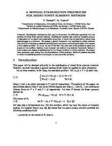
The phase field (PF) approach to phase transformations (PTs) dates back to Landau, who introduced the order parameters related to the symmetry of the phases, and also to Ginzburg, who introduced a gradient-based interfacial energy (see e.g. [1] for a review). This approach is popularly known as the Ginzburg-Landau theory, which is also similar to the Allen-Cahn approach [2]. The PF approaches of the Ginzburg-Landau type have been extensively used to study a wide range of physical problems such as solid↔melt transitions (see [3–10] and the references therein), grain growth (see [11–16] and the references therein), evolution of domain structures (see e.g. [12, 17, 18]), martensitic transformations (MTs) [19–34], and interaction between MTs and plasticity [35–37]. Our focus in this paper will be mainly on MT, which is a diffusion-less, displacive process with dominating shear deformation. Such transformation yields the shape memory effect, ferroelectricity, and magnetoelasticity in various alloys [38, 39]. Complex microstructures are formed within the materials undergoing MTs, which usually include laminated structures consisting of martensitic (M) plates of alternative variants called twinned martensite, as well as twins within twins, wedge, etc. [38, 40], which usually consist of austenite (A) and all possible martensitic variants Mi (i = 1, 2, . . . , N , and N is the number of variants). One should also note that all of the A-M and variant-variant interfaces possess finite energy and are subjected to biaxial stresses, which act in a plane tangential to the interface [41]; the schematic is shown in Fig. 1 when the elastic stresses are neglected. Such stresses play a very important role in the nucleation and propagation of the interfaces [42, 43]. According to the Shuttleworth equation, the total ¯ = σ ¯ st + σ ¯ e = γ(I − n ⊗ n) + ∂γ/∂¯ interfacial stress tensor σ ε (a tangential tensor) is composed of ¯ e = ∂γ/∂¯ ¯, and a structural an elastic part σ ε that depends on the strain tensor within the interface, ε ¯ st = γ(I − n ⊗ n), where n is the unit normal to the interface, γ is the interfacial energy, I part, σ is the identity tensor, and ⊗ denotes the dyadic product. Within the phase field models where the interfaces are finite-width regions, the elastic part of the interfacial stresses arises naturally due to the elastic strains. To introduce the other part, i.e. the structural stress tensor, Levitas and coworkers [20, 21, 29, 44] multiplied the double-well barrier energy and the gradient energy in the Helmholtz’s free energy by the determinant of the total deformation gradient tensor, and considered the gradient of the order parameters in the deformed configuration. When the structural stresses are considered, the tangent modulus for the mechanical equilibrium equations would obviously have contributions from both the elastic

3

γ

γ

γ γ Figure 1: Schematic of an arbitrary finite-width interface subjected to biaxial interfacial structural stresses, where γ is the magnitude of the stress acting in the tangent plane of the interface. The elastic interfacial stresses are not shown here. response and the structural stresses in both finite strain and small strain models [21, 45]. The structural stresses obviously depend on nontraditional mechanics parameters (gradient of the order parameters in the deformed configuration). We are not aware of any algorithmic treatment for the models with structural interfacial stresses as it is done in the current paper. Note that it is very important to have the correct expressions for the tangent modulus for both mechanics and PF problems, at least for a good convergence within the Newton’s iterations. All the PF approaches introduce order parameters which describe the phases. The interfaces are of finite width and have well-defined structures. The volume fraction (e.g. [4, 24, 26, 46]) or transformation strain-based order parameters (e.g. [30, 32]) are usually used. In this paper, the transformation strainrelated order parameters, which describe the change in symmetries (the PT process) in a continuous way, are considered. A system of Ginzburg-Landau equations governs the evolution of the order parameters, which are highly-nonlinear parabolic partial differential equations (PDEs). When the PT phenomenon is stress- and temperature-induced, the mechanical equilibrium equations also play a non-trivial role and are coupled to the system of Ginzburg-Landau equations. The finite element method (FEM) has been used in this paper to solve the coupled PF and equilibrium equations. FEM is preferred over the finite difference method (see e.g. [3, 7, 47], where this approach was used), as FEM can efficiently handle any arbitrary domain shape, whereas the other method cannot. Pioneering work in the simulations of PF equations for MTs was done by Khachaturyan and coworkers [32, 33], who used the Fourier Transform method to numerically solve the coupled PDEs. Other groups of researchers used similar approaches; see e.g. Roytburd and coworkers [18], Chen and coworkers [12, 34], Lei et al. [22], Vidyasagar et al. [48], Kundin et al. [37] etc. The spectral methods are much faster, but they can only handle problems with periodic boundary conditions. Hence, the Fourier method cannot be used for models which consider the surface effects; see e.g. [44], where FEM was used.

4 In solving the PF equations for MTs, FEM has been used by a limited number of groups, e.g. Levitas and coworkers [20, 21, 44, 49–51], Clayton and Knap [27, 28], Stupkiewicz and coworkers [25, 26], Hildebrand and Miehe [24], She at al. [52], Paranjape et al. [35]. Finite strain theories were considered in [24–28, 50, 51], but the rest of the works dealt with small strain theories. A detailed FE formalism for stress- and temperature-induced MTs at finite strains and with interfacial stresses is still missing. Even a coherent FE procedure for the models considering small strain and/or neglecting the interfacial stresses is not yet available, to the best of our knowledge. Our goal in this paper is to present a rigorous FE formalism for the coupled PF equations and the mechanics equations related to the model developed in [45] for multivariant MTs induced by stresses and temperature at finite strains and with interfacial stresses. To illustrate the formalism, we solve some problems showing complex microstructure evolutions and compare the numerical results for two problems with the known analytical solutions. Formulations for a system with A and N martensitic variants have been presented. The weak forms for the equilibrium equation and the Ginzburg-Landau equations, where a non-monolithic approach is used, are established using the variational method. The time derivative in the PF equations is discretized mainly by using a backward difference scheme of order two (BDF2). The mechanics problem and the PF equations have been solved using the Newton’s iterative methods, for which the weak forms are linearized and the corresponding tangent moduli for the mechanics and PF problems are obtained. The tangent modulus related to the mechanics problem is a fourth order tensor that is decomposed into two parts, which are related to the elastic and structural stresses, respectively. An adaptive time stepping has been used to integrate the PF equations. Based on the FE formulation, we have developed an FE code in an open source deal.II and solved the following three problems: (i) Evolution of microstructure in a system with A and single M variant in a rectangular parallelepiped. (ii) Twinning in a system with A and two variants M1 and M2 under the generalized plane strain condition. The effect of sample size on the twinned microstructure is also studied. (iii) Nanoindentation of a rectangular sample under plane stress condition. Two different kinematic models (KMs) for the transformation deformation gradient tensor F t are considered: in KM-I, F t is taken as a linear combination of the Bain strains, which are multiplied by the interpolations functions [29, 31], and in KM-II, we take F t as the exponential of a linear combination of the natural logarithm of the Bain tensors multiplied by the interpolation functions [25, 26]. For each problem, the results for both KM-I and KM-II are presented and compared. We have also compared the elastic stresses within the twin boundaries for these two KMs. We report that the elastic stress component in the longitudinal direction of the twin boundaries is much larger for KM-II

5 than KM-I, which is in agreement with our recent analytical and numerical study on interfacial stresses in [53]. The performance of our adaptive time stepping scheme is also analyzed. The content of the paper is as follows: the system of governing equations is listed in Section 2; the weak forms of the governing PDEs and their linearizations are presented in Section 3; FE discretization details and the computational algorithm are given in Section 4; various material parameters are derived and listed in Section 5; Section 6 presents the numerical examples; finally, the conclusions of the study are drawn in Section 7. Notation. We denote the inner product and multiplication between two second order tensors as A : B = Aab Bba and (A·B)ab = Aac Bcb , respectively, where the repeated indices denote Einstein’s summation, and Aab and Bab are the components of the tensors in a right-handed orthonormal Cartesian basis {e1 , e2 , e3 }. √ The Euclidean norm of A is denoted as |A| = A : AT ; I denotes the second order identity tensor; δab denotes the Kronecker delta; A−1 , AT , det A, tr A, sym(A), and skew(A) denote the inversion, transposition, determinant, trace, symmetric part, and skew part of A, respectively. The symbols ∇0 and ∇ represent the gradient operators in the reference (undeformed) Ω0 and current (deformed) Ω configurations, respectively; ∇20 := ∇0 · ∇0 and ∇2 := ∇ · ∇ are the Laplacian operators in Ω0 and Ω, respectively. The symbol := stands for equality by definition.

2

System of coupled mechanics and phase field equations

Recently, Basak and Levitas [45] developed a novel multiphase phase field model for studying stress and temperature-induced MTs for a system with austenite and N martensitic variants considering N + 1 order parameters η0 , η1 , . . . , ηi , ηj , . . . , ηN . The order parameter η0 describes A ↔ M transformations such that η0 = 0 in A and η0 = 1 in M. The order parameter ηi (for i = 1, . . . , N ) describes the variant Mi such that ηi = 1 in Mi and ηi = 0 in Mj for all j 6= i. Also, η1 , . . . , ηN satisfy the constraint (see [45] for details) N X

ηi = 1.

(2.1)

i=1

In this section we enlist the system of coupled elasticity and phase field equations for an N -variant system; see [45] for their derivation. The reference, stress-relaxed intermediate, and current configurations are denoted by Ω0 , Ωt , and Ω, respectively. The external boundaries in Ω0 and Ω are denoted by S0 and S, respectively. We designate the traction boundary (Neumann boundary) in Ω0 by S0T and the displacement boundary (Dirichlet boundary) by S0u , such that S0 = S0u ∪ S0T . Similarly, for the PF equations S0 = S0ηk ∪ S0Tk for all k = 0, 1, . . . , N , where S0ηk is the Dirichlet boundary where ηk is

6 specified, and S0Tk is the Neumann boundary corresponding to the order parameter ηk .

2.1

Kinematics

We denote the position vector of a particle in Ω by r(r 0 , t), where r = r 0 + u(r 0 , t), r 0 is the position vector in Ω0 , u is the displacement vector, and t denotes time. We assume that both u, and hence, r are sufficiently smooth functions of r 0 and t. The total deformation gradient F is decomposed into [29] F := ∇0 r = F e · F t = V e · R · U t ,

(2.2)

where the subscripts e and t denote elastic and transformational parts, respectively; F e = V e · Re and F t = Rt · U t are, respectively, the elastic and transformational parts of F ; U t is the right transformation stretch tensor (symmetric); V e is the left elastic stretch tensor (symmetric); Rt and Re are the rotation tensors; and R = Re · Rt is the lattice rotation tensor. We also define J = det F := dV /dV0 , Jt = det F t := dVt /dV0 , and Je = det F e := dV /dVt , where dV0 , dVt , and dV are infinitesimal volume elements in Ω0 , Ωt , and Ω, respectively. Hence by Eq. (2.2), J = Jt Je . The Lagrangian total and elastic strains are defined as E := 0.5(C − I),

and E e := 0.5(C e − I),

(2.3)

respectively, where C = F T · F and C e = F Te · F e are the right Cauchy-Green total strain and elastic strain tensors, respectively. Also, the Eulerian total and elastic strain tensors are b = 0.5(B − I) and be = 0.5(B e −I), respectively, where B = F ·F T = V 2 and B e = F e ·F Te = V 2e are the left Cauchy-Green √ total strain and elastic strain tensors, respectively. Note that V = B is the left total stretch tensor. Kinematic models for F t . Two KMs for the transformation deformation gradient tensor F t have been assumed. In KM-I we express F t as (see [45] for details) for KM-I:

F t = Ut = I +

N X

εti ϕ(aε , η0 )φi (ηi );

(2.4)

i=1

where εti = U ti − I and U ti are the Bain strain tensor and Bain stretch tensor, respectively, for Mi . The interpolation functions ϕ(aε , η0 ) and φi (ηi ) are taken as [45] ϕ(aε , η0 ) = aε η02 + (4 − 2aε )η03 + (aε − 3)η04 ,

and φi (ηi ) = ηi2 (3 − 2ηi ),

(2.5)

respectively, and 0 ≤ aε ≤ 6 is a constant parameter. The interpolation function ϕ(aε , η0 ) satisfies the ∂ϕ(aε , 0) ∂ϕ(aε , 1) conditions ϕ(aε , 0) = 0, ϕ(aε , 1) = 1, and = = 0; and φi satisfies φi (0) = 0, φi (1) = 1, ∂η0 ∂η0 ∂φi (ηi = 0) ∂φi (ηi = 1) and = = 0 for all i = 1, 2, . . . , N . This KM (Eq. (2.4)) was introduced and used ∂ηi ∂ηi

7 in [20, 21, 29, 31, 45, 50, 51]. It should be noted that although the specific volumes of the variants are the same, each variant↔variant transformation path, i.e. Mi ↔ Mj for all i 6= j, is not isochoric in KM-I [45]. In the other model KM-II, we take F t as (see [45] for details) " # N X for KM-II: F t = U t = exp ϕ(aε , η0 ) φi (ηi ) ln U ti .

(2.6)

i=1

The definitions and properties of the exponential and logarithm of a second order tensor can be found in, e.g., [54, 55]. It was proved in [45] that each Mi ↔ Mj transformation (for all i 6= j) given by Eq. (2.6) is isochoric for the entire transformation path. Note that in KM-I and KM-II, F t are symmetric and taken to be identical to the symmetric tensor U t and Rt is assumed to be Rt = I. There are cases where the transformation deformation gradient can be nonsymmetric, such as the simple shear-based kinematic model considered in [45, 53]. Thus to derive a general FE formulation which is applicable for both symmetric and nonsymmetric F t , we would continue to designate the transformation rules (2.4) and (2.6) for KM-I and KM-II as F t .

2.2

Free energy

We consider the Helmholtz free energy per unit mass of the body in the following form [29, 45]: ψ(F , θ, η0 , ηi , ∇η0 , ∇ηi ) =

Jt ψe (F e , θ, η0 , ηi )+J ψ˘θ (θ, η0 , ηi )+ ψ˜θ (θ, η0 , ηi )+ψp (η0 , ηi )+Jψ ∇ (η0 , ∇η0 , ∇ηi ) ρ0 (2.7)

for all i = 1, 2, . . . , N , where ψ e is the elastic strain energy per unit volume of Ωt , ψ˘θ is the barrier energy related to A ↔ M and all the Mi ↔ Mj transformations, ψ˜θ is the thermal energy, ψ ∇ is the interfacial energy, and ψ p penalizes various junctions between A and the variants. It should be noted that in Eq. (2.7) the barrier energy and the gradient energy are multiplied by J and the gradients of η0 and ηi are expressed in the deformed configuration. This yields the desired form of the structural stresses (here given by Eqs. (2.17) and (2.18)) as discussed in Section 1; see [29] for further details. The material properties at each material point are determined using [45] M (η0 , ηi , θ, F ) = M0 (1 − ϕ(a, η0 )) + ϕ(a, η0 )

N X

Mi φi (ηi ),

(2.8)

i=1

where M0 and Mi are the properties of the phases A and Mi , respectively, ϕ(a, η0 ) is an interpolation function and has the same functional form of ϕ(aε , η0 ) given by Eq. (2.5)1 when aε is replaced by the constant parameter a. Note that ϕ(a, η0 ) also satisfies the conditions similar to those of ϕ(aε , η0 ) discussed above. Evidently, the interpolation Eq. (2.8) yields the property of the corresponding phase (A or Mi )

8 when the appropriate values of the order parameters are assigned. The explicit form of all of the energies is [45] ψe =

1 ˆ e (η0 , ηi ) : E e , Ee : C 2

ˆ e (η0 , ηi ) = (1 − ϕ(a, η0 ))C ˆ (e)0 + ϕ(a, η0 ) where C

˜ ψ˘θ = [A0M (θ) + (aθ − 3)∆ψ θ (θ)] η02 (1 − η0 )2 + Aϕ(a b , η0 ) ψ˜θ = ψ0θ (θ) + η02 (3 − 2η0 ) ∆ψ θ (θ) ψp =

N −1 X

N X

i=1 j=i+1

[1 − ϕ(aK , η0 )]

N X

N X

K0ijk η02 ηi2 ηj2 ηk2 +

i=1 j=i+1 k=j+1

ˆ (e)i ; φi (ηi )C

(2.9)

i=1

ηi2 ηj2 ;

(2.10)

i=1 j=i+1

where ∆ψ θ = −∆s0M (θ − θe );

Kij (ηi + ηj − 1)2 ηi2 ηj2 + [1 − ϕ(aK , η0 )] N −2 N −1 X X

N −1 X

N X

N −1 X

N X

(2.11)

K0ij η02 ηi2 ηj2 +

i=1 j=i+1

N −3 N −2 X X

N −1 X

N −2 N −1 X X

N X

Kijk ηi2 ηj2 ηk2 +

i=1 j=i+1 k=j+1 N X

Kijkl ηi2 ηj2 ηk2 ηl2 ,

where

i=1 j=i+1 k=j+1 l=k+1

Kii = K0ii = Kiji = Kiik = K0iji = K0iik = Kijil = Kiikl = Kijjl = Kijki = Kijkk = 0; ψ∇ =

N −1 X N X
1 β0M |∇η0 |2 + ϕ(η ˜ 0 , aβ , ac ) βij |∇ηi |2 − 2∇ηi · ∇ηj + |∇ηj |2 , 2ρ0 8ρ0

(2.12)

where βii = 0,

(2.13)

i=1 j=i+1

ϕ(a ˜ β , ac , η0 ) = ac +

aβ η02

− 2[aβ − 2(1 − ac )]η03 + [aβ − 3(1 − ac )]η04 .

(2.14)

ˆ e (η0 , ηi ) is the fourth-order elastic All of the symbols used in Eqs. (2.9) to (2.14) are now defined. C ˆ (e)0 and C ˆ (e)i are the elastic modulus tensors of A0M and Mi , modulus tensor for a material point; C respectively; A0M > 0 is the barrier height between A and M; A˜ > 0 is the barrier height between Mi and θ − ψ θ is the thermal energy difference between Mj for all i 6= j; ψ0θ is the thermal energy of A; ∆ψ θ = ψM 0

M and A; ∆s0M = sM − s0 is the change in entropy due to A to M transformation (s0 and sM denoting the entropy of A and M, respectively); θ > 0 is the absolute temperature; θe is the thermodynamic equilibrium temperature between A and M; Kij ≥ 0 is a controlling parameter for penalizing the deviation of the transformation path (i.e. Mj ↔ Mi path) from the straight line ηj + ηi = 1 for all ηk = 0 and k 6= j, i; K0ij ≥ 0, Kijk ≥ 0, K0ijk ≥ 0, and Kijkl ≥ 0 are the constant coefficients for penalizing the junctions between A-Mi -Mj , Mi -Mj -Mk , A-Mi -Mj -Mk , and Mi -Mj -Mk -Ml , respectively; β0M > 0 and βij > 0 are the energy coefficients for A-M and Mi -Mj interfaces, respectively; ρ0 is the density of the solid in Ω0 ; and ab , aK , aβ , ac are the material parameters.

2.3

Mechanical equilibrium equations and stresses

Neglecting the body forces and inertia we write the mechanical equilibrium equations as [29, 45] ∇0 · P = 0

in Ω0 ,

or ∇ · σ = 0 in Ω,

(2.15)

9 where P is the total first Piola-Kirchhoff stress tensor and σ is the total Cauchy stress tensor. These tensors are decomposed into their elastic and structural parts [45] P = P e + P st and σ = σ e + σ st . Here, the subscripts e and st denote elastic and structural parts, respectively. In general, the elastic first Piola-Kirchhoff and Cauchy stresses are given by [29, 45] ˆ e = ∂ψe (E e ) . where S ∂E e

(2.16)

For isotropic elastic response, P e and σ e can alternatively be expressed as P e = Jt V 2e ·

∂ψe (be ) · F −T ∂be

ˆ e · F −T ; P e = Jt F e · S t

and σ e = Je−1 V 2e ·

ˆe · FT, σ e = Je−1 F e · S e

∂ψe (be ) , respectively. The first Piola-Kirchhoff structural stress tensor is [45] ∂be

P st = Jρ0 (ψ˘θ + ψ ∇ )F −T − Jβ0M ∇η0 ⊗ ∇η0 · F −T − J ϕ˜

N X N X βij i=1 j=1

4

∇ηi ⊗ (∇ηi − ∇ηj ) · F −T .

(2.17)

Noticing that [45] βij = βji and βii = 0 (for all i 6= j), the structural part of σ is expressed as σ st = ρ0 (ψ˘θ +ψ ∇ )I −β0M ∇η0 ⊗∇η0 − ϕ˜

N −1 X

N X βij [∇ηi ⊗∇ηi +∇ηj ⊗∇ηj −2sym(∇ηi ⊗∇ηj )]. (2.18) 4

i=1 j=i+1

When A-M and Mi -Mj interfaces are considered, Eq. (2.18) simplifies as σ st = σ(st)0M (I − k0M ⊗ k0M ), σ(st)0M

and σ st = σ(st)ij (I − kij ⊗ kij ),

= β0M |∇η0 |2 = 2ρ0 ψ˘θ , σ(st)ij = βij |∇ηi |2 = 2ρ0 ψ˘θ , k0M =

respectively, where

∇ηi ∇η0 , and kij = (, 2.19) |∇η0 | |∇ηi |

i.e. for each interface, Eq. (2.18) yields biaxial tension where the resultant force is equal to the interface energy γ (see [29] for the proof), similar to that in the sharp interface theory [41].

2.4

Ginzburg-Landau equations

The Ginzburg-Landau equations for all N + 1 order parameters are (see [45] for the derivation) η˙ 0 = L0M X0 ,

and η˙ i =

N X j=1,6=i

Lij (Xi − Xj )

for i = 1, 2, . . . , N,

(2.20)

10 where L0M and Lij are the kinetic coefficients for A-M and Mi -Mj interfaces, respectively, and X0 and Xi are the conjugate forces for the evolution of the order parameters η0 and ηi , respectively: X0 =

N −1 X N X
∂ϕ(ab , η0 ) ∂F t ∂ψe 2 θ ˜ P Te · F − Jt ψe I : F −1 · − J − − ρ (6η − 6η )∆ψ − Jρ A ηi2 ηj2 t 0 0 0 0 t ∂η0 ∂η0 F e ∂η0 i=1 j=i+1

N X ˜ β , ac , η0 ) J ∂ ϕ(a βij |∇ηi − ∇ηj |2 − 8 ∂η0 i=1 j=i+1    N X ∂ϕ(aK , η0 ) 2 2 2 2 η0 + K0ijk ηi ηj ηk 2(1 − ϕ(aK , η0 ))η0 − ∂η0

Jρ0 [A0M (θ) + (aθ − 3)∆ψ θ (θ)](2η0 − 6η02 + 4η03 ) − 

N −1 X

ρ0 

N X

K0ij ηi2 ηj2 +

i=1 j=i+1

∇0 · Jβ0M F

−1

N −2 N −1 X X

N −1 X

i=1 j=i+1 k=j+1




· ∇η0 ;

(2.21)

N N X X ∂ψe ∂F t 2 ˜ · F − Jt ψe I : = · − Jt − 2Jρ A ϕ(a , η ) − 2ρ η η Kij (ηi + ηj − 1) × 0 0 i j b 0 ∂ηi ∂ηi F e j=1 j=1,6=i   N N −1 N N −1 X N X X X X 2 2 2 2 2  (2ηi + ηj − 1)ηj ηi − 2ρ0 K0ij ηj + K0ijk ηj ηk η0 ηi (1 − ϕ(aK , η0 )) − 2ρ0 Kijk × P Te

Xi




F −1 t

j=1

ηi ηj2 ηk2 − 2ρ0

N −2 N −1 X X

N X

j=1 k=j+1 l=k+1

j=1 k=j+1

j=1 k=j+1

 ˜ β , ac , η0 )J Kijkl ηi ηj2 ηk2 ηl2 + ∇0 · ϕ(a

N X βij j=1

4

 F −1 · (∇ηi − ∇ηj )

for all i = 1, 2, 3, . . . , N. Note that X0 and Xi , which are given by Eqs. (2.21) and (2.22), respectively, are the functions of all of the N + 1 order parameters η0 , η1 , η2 , . . . , ηN . Because the N order parameters η1 , . . . , ηN are related through the constraint (2.1), out of the N Ginzburg-Landau equations in Eq. (2.20)2 , only N − 1 are independent. This can be verified simply by taking the time derivative in Eq. (2.1). Thus, it is sufficient to solve N − 1 Ginzburg-Landau equations for the order parameters related to the variants, and the other order parameter can be determined by using Eq. (2.1). The modified N independent Ginzburg-Landau equations are listed in the Appendix A.

2.5

Boundary conditions

Mechanics problem. On the traction boundary S0T , the traction is specified (denoted by psp ), and on the displacement boundary S0u , the displacements are specified (denoted by usp ): P · n0 = psp on S0T , and u = usp on S0u . The mixed boundary conditions where, on a single surface, some components of displacements are specified and some components of the traction are specified, are used in some cases. Phase field problem. For the order parameters, we consider the homogeneous Neumann boundary conditions on S0Tk and specify the order parameter ηk on the respective Dirichlet boundary S0ηk [29, 45]:

(2.22)

11 ∇ηk ·n = 0 on S0Tk , and ηk = ηksp on S0ηk for all k = 0, 1, 2, . . . , N . The homogeneous Neumann boundary conditions in a sample are the consequence of the assumption that the external surface energy does not change during phase transformation [29]. The exact boundary conditions for each problem at hand will be specified in Section 6, where they will be discussed in detail.

3

Weak forms of the governing equations and their linearizations

Assuming the total Lagrangian approach (see e.g. Chapter 8 of [56]), we now derive the weak forms for the equilibrium equation given by Eq. (2.15)1 or (2.15)2 and N independent Ginzburg-Landau equations listed in Appendix A. A non-monolithic strategy has been considered, and the equilibrium equations and all of the phase field equations are solved in a decoupled manner. While solving for the displacements, the order parameters are assumed to remain constant, and while solving for the order parameters during a time step, the total deformation gradient tensor is kept constant. We denote the weighting function (also called the test function or virtual displacements) for the displacements by δu, which is sufficiently smooth and satisfies δu = 0 on the displacement boundary S0u . The sufficiently smooth test function for each of the order parameters is denoted by δηk such that δηk = 0 on the corresponding order parameter boundary S0ηk for all k = 0, 1, 2, . . . , N . Only the main results are discussed in this section. The detailed derivation is shown in Appendix B.

3.1

Equilibrium equations: weak form and linearization

The weak form of the mechanical equilibrium equation Eq. (2.15) is (see for example, [57, 58]) Z R(u, δu) = − (∇0 · P ) · δu dV0 = 0,

(3.1)

Ω0

which is also known as the principle of virtual work (see e.g. Chapter 3 of [57]). For a given material and the displacement and traction boundary conditions, our objective is to solve for the displacements satisfying the weak form given by Eq. (3.1), which can be rewritten as (see Appendix B for derivation) Z Z Z Z sp R(u, δu) = S : δE dV0 − p · δu dA0 = τ : δε dV0 − psp · δu dA0 = 0, (3.2) Ω0

S0T

Ω0

S0T

where S is the second Piola-Kirchhoff stress, τ = Jσ is the Kirchhoff stress, psp is the specified traction on S0T , and δE and δε are the variations of E and ε given by δE = F T · δε · F and δε := 0.5(∇δu + ∇δuT ); see Chapter 10 of [58]. We will use the Newton’s iteration method to find the solution, and thus must linearize Eq. (3.2) in the direction of an increment of the displacement vector denoted by ∆u. Two approaches are generally

12 used in this process [57, 59]: (i) in one approach, the weak form, i.e. Eq. (3.2), is discretized and then linearized with respect to the nodal displacements; (ii) in the other approach, at first the weak form is linearized and the resulting equation is then discretized. We will adopt the latter approach here. Note that this latter approach may not work in some cases where nonstandard discretizations are used; see e.g. [59]. Assuming that the external loads are ‘dead’, i.e. psp is independent of u, we linearize R (assumed to be a differentiable functional of u) in Eq. (3.1) to obtain (see Appendix B for the derivation) Z Z ∆R · ∆u = JC : ∆ε : δε dV0 + ∇∆u · τ : ∇δuT dV0 , where Ω0

(3.3)

Ω0

C = Ce + Cst

(3.4)

is the fourth order total modulus tensor in the deformed configuration composed of the elastic part Ce and the structural part Cst which are given by Ce = Cst =

1 1 ˆ e : (F e  F e )T , and (F  F ) : C e : (F  F )T = (F e  F e ) : C J Je 1 [τ st ⊗ I + I ⊗ τ st − 2(τ st  I + I  τ st ) : S + ρ0 J(ψ˘θ + ψ ∇ )(2S − I ⊗ I)], J

(3.5)

respectively. In Eq. (3.3), ∆(·) denotes the increment of the function within the argument. Note that in ˆ e is the fourth order elastic modulus tensor with respect to Ωt : Eq. (3.5)1 , C 2 ˆ ˆ e := ∂ S e = ∂ ψe . C ∂E e ∂E e ∂E e

(3.6)

In Eq. (3.5)2 , τ st denotes the structural part of τ ; see Appendix B for the definitions of the products between the second order tensors denoted by ⊗ and , fourth order symmetrizer S, and transpose of a fourth order tensor. The fourth order elasticity and structural tensors can be expressed in the indicial notations as C(e)abcd =

1 1 FaA FbB FcC FdD C(e)ABCD = F(e) aAˆ F(e) bBˆ F(e) cCˆ F(e) dDˆ Cˆ(e)AˆBˆ Cˆ Dˆ , J Je

and

JC(st)abcd = τ(st)ab δcd + δab τ(st)cd − (τ(st)ac δbd + τ(st)ad δbc + δac τ(st)bd + δad τ(st)bc ) + ρ0 J(ψ˘θ + ψ ∇ )(δac δbd + δad δbc − δab δcd ),

(3.7)

respectively, where, following Zienkiewicz and Taylor [58], we use the indices in capital letters (i.e. A, B, C, D etc.) for Ω0 , and the indices in lower case (i.e. a, b, c, d etc.) for Ω. The indices with ˆ B, ˆ C, ˆ D ˆ etc.) are used for Ωt . ‘hat’ (i.e. A, ˆ e , and Ce and the structural tensor Cst possess both minor and Notably, all of the elasticity tensors C e , C major symmetries: e.g. C(e)ABCD = C(e)BACD = C(e)ABDC (minor symmetry), and C(e)ABCD = C(e)CDAB

13 (major symmetry); see e.g. Chapter 6 of [56] for the definitions. Consequently, C also possess those symmetries. For solids, Cˆe is known either from experiments or from atomistic calculations, and hence it is considered as a material property (see Eq. (2.9)). Obviously, for any material point, C e and Ce depend not only on Cˆe , but also on the present state of deformation. The relation between Ce and C e in Eq. (3.5)1 is well-known in nonlinear elasticity (see e.g. Chapter 6 of [56]), but to the best of our knowledge, ˆ e in Eq. (3.5)1 appear here for the first time. Obviously, if the relations between these tensors and C the interfacial stresses are neglected, i.e. the barrier and gradient energies in the Helmholtz free energy given by Eq. (2.7) are not multiplied by J and the gradient of the order parameters are taken in Ω0 , σ st identically vanishes and so does Cst . The last integral in Eq. (3.3) contributes to the total tangent stiffness matrix, which is also called the geometric stiffness (see Section 4 below, as well as e.g. [57, 58]). Note that the contribution of this integral has arisen due to the geometric nonlinearity, and it is thus neglected in the small strain FE formulations [60]. Note that the integrands of the weak form R (given by Eq. (3.2)2 ) and its linearization ∆R ·∆u (given by Eq. (3.3)) are all expressed in terms of the stresses, strains, and tangent modulus in the deformed configuration Ω, whereas the integrations are performed in the reference body Ω0 . This approach has an advantage over the one in which the integrands are expressed in Ω in that the computation of the standard B f e matrix (in FEM) is much simpler. In fact, the B f e matrix in this case turns out to be identical to the matrix used in the small strain calculations (see [57] and Chapter 10 of [58] for details).

3.2

Ginzburg-Landau equations: time discretization, weak form, and linearization

We now derive the weak forms of N independent Ginzburg-landau equations listed in Eq. (A.1), which were obtained using the original N + 1 equations given by Eq. (2.20). We discretize the time derivative of the order parameters using a backward difference scheme over a time period t ∈ [t0 , tf ] and then write the weak forms, where t0 and tf denote the initial and final time instances, respectively. An A-stable backward difference scheme of order two (BDF2) is used to discretize the time derivatives (see [61] for details of the scheme). Such a scheme requires solutions from the two consecutive previous time steps. Thus, for the first time step, we use BDF1 scheme (first order backward difference scheme), which requires the solution from the previous time step only (which will be provided by the initial conditions). Then, from the second step onwards, the BDF2 scheme is used. For the BDF1 or BDF2 scheme, η˙ k is

14 discretized as [61] η˙ k =

c1 ηkn + c2 ηkn−1 + c3 ηkn−2 ∆tn

for k = 0, 1, . . . , N,

(3.8)

where for BDF1, c1 = 1, c2 = −1, and c3 = 0, and for BDF2, c1 = 1.5, c2 = −2, and c3 = 0.5. In Eq. (3.8), the superscript n = 0, 1, 2, . . . denotes the index for time such that the time instance after nth time iteration is tn+1 = tn +∆tn , and ∆tn denotes the accepted time step size leading to the converged solutions for the order parameters in our adaptive time stepping scheme. Discretizing the N independent equations from Eq. (A.1) by using Eq. (3.8), the finite difference forms of the kinetic equations are obtained and are then multiplied by the weighted function δηkn , integrated over the entire domain to obtain the weak forms corresponding to N independent Ginzburg-Landau equations, which can be expressed in the following general form (see Appendix B.2 for derivation) Rk = c1

Z

ηkn δηkn dV0

+ ∆t

n

Ω0

Ω0

Z c2 Ω0

Z

ηkn−1 δηkn dV0

Z + c3 Ω0

Lβk J n χnk

(F

n−1

·F

ηkn−2 δηkn dV0 = 0

n−T

·

∇0 ηkn )

·

∇0 δηkn dV0

+ ∆t

n

Z

fkn δηkn dV0 +

Ω0

for k = 0, 1, . . . , N − 1.

(3.9)

To obtain Eq. (3.9), we have used the Gauss divergence theorem and the Nanson’s formula n dS = JF −T · n0 dS0 [56], applied the homogeneous Neumann boundary condition on the entire boundary (see Section 2.5), and assumed that all of the kinetic coefficients are spatially constants. In Eq. (3.9), P n ˜ β , ac , η0 ) for all k = 1, 2, . . . , N − 1. The Lβ0 = L0M β0M , χn0 = 1, Lβk = N m=1,6=k Lkm βkm , and χk = ϕ(a expressions for f0n and fin (for all i = 1, . . . , N − 1) are listed in Appendix B.2 and given by Eqs. (B.28) and (B.40), respectively. We use the Taylor expansion of the weak forms about ηkn , i.e. Rk (ηkn + ∆k ηkn , δηkn ) = Rk (ηkn , δηkn ) + ∆k Rk + o(∆k ηkn ) = 0

for k = 0, 1, . . . , N − 1,

(3.10)

to obtain the tangent matrix, where the increment of a function (or functional) with respect to ηk is denoted by ∆k , and Z Z ∂Rk n n n n ∆k Rk = ∆ η = c ∆ η δη dV + ∆t Lβk χnk J n βk (F n−1 · F n−T · ∇0 ∆k ηkn ) · ∇0 δηkn dV0 + 1 0 k k k k k ∂ηkn F Ω0 Ω0 Z n ∂f n n k for k = 0, 1, . . . , N − 1. (3.11) ∆tn n ∆k ηk δηk dV0 ∂η Ω0 k F The complete expressions for (∂f0n /∂η0n )F and (∂fkn /∂ηkn )F are given by Eqs. (B.41) and (B.42), respectively. Note that the derivatives of the weak forms have been calculated while keeping F fixed within our non-monolithic formulation, as we assume that the state of deformation within the body remains fixed

15 while the order parameters are evolving.

4

Finite element implementation

We discretize the reference configuration Ω0 (i.e. the initial body) into nel number of isoparametric el el Ωel elements, i.e. Ω0 ≈ ∪nel=1 0 , and consider the following interpolations in element Ω0 (also see [57]):

r el 0 =

ng X

Nι (ξ)˜ r 0ι ,

r el =

ng X

el

∆u =

Nι (ξ)∆˜ uι ,

ηkel

=

ng X

Nι (u)˜ uι ,

ng X

Nι (ξ)˜ ηk ι ,

δηkel

=

˜ ι, Nι (ξ)δ u

ι=1 ng X

Nι (ξ)δ η˜k ι ,

∆k ηkel

=

ng X

Nι (ξ)∆k η˜k ι ,

ι=1

ι=1

ι=1

ι=1

ng X

δuel =

ι=1

ι=1

ι=1 ng

X

uel =

Nι (ξ)˜ rι ,

for all k = 0, 1, . . . , N − 1,

(4.1)

where Nι (ι = 1, 2, . . . , ng ) are the shape functions corresponding to the element Ωel 0 ; ng is the number of grid points in each element; the quantities with tilde correspond to the nodal values, i.e., for example, ˜ ι denotes the displacement vector at ιth node; ξ denotes the coordinates of the isoparametric reference u element (see e.g. Chapter 4 of [57]); and the superscript el denotes the index for the finite elements. The deformation gradient tensor in Ωel 0 can hence be expressed as (see e.g. Chapter 4 of [57]) F

el

el

=j ·J

el −1

ng

,

where J

el

∂r 0 el X = = r˜0ι ⊗ ∇ξ Nι , ∂ξ ι=1

ng

∂r el X j = = r˜ι ⊗ ∇ξ Nι , ∂ξ el

(4.2)

ι=1

and ∇ξ denotes the gradient operator in the coordinate of the isoparametric element. Denoting the local coordinate system of the reference element in our isoparametric mapping by ξ = {ξ1 , ξ2 , ξ3 }T , we can write ∇ξ Nι = [Nι,ξ1 , Nι,ξ2 , Nι,ξ3 ]T , where the subscripts followed by a comma designate the derivative with respect to the corresponding isoparametric coordinate. The spatial gradients of the displacement and the order parameters, as well as the gradients of their weighting functions and increments take the form (see e.g. Chapter 4 of [57]): el

∇u

=

ι=1 ng

∇ηkel =

4.1

ng X

X ι=1

˜ι ⊗ j u η˜k ι j el

el −T

−T

· ∇ξ Nι ,

· ∇ ξ Nι ,

el

∇δu = ∇δηkel =

ng X ι=1

ng X ι=1

˜ι ⊗ j δu

δ η˜k ι j el

el −T

−T

· ∇ξ Nι ,

· ∇ξ Nι ,

el

∇∆u =

∇∆k ηkel =

ng X ι=1

ng X ι=1

∆˜ uι ⊗ j el

∆k η˜k ι j el

−T

−T

· ∇ ξ Nι ;

· ∇ξ Nι(4.3) .

Discretization of the equilibrium equation

We now use Eq. (3.2) in Eq. (B.3), discretize the resulting equations using Eqs. (4.1)-(4.3) while neglecting the higher order terms in ∆u from Eq. (B.3), apply the standard assembly operation, and

16 then use the arbitrariness of the global weighting vector (nodal) to finally obtain the system of algebraic equations given by Eq. (4.4) in Box-I (also see [57, 59]). Note that ∆up is the nu × 1 incremental displacement matrix at the pth iteration; K and r u are the nu × nu symmetric global tangent matrix and nu × 1 residual vector defined by Eqs. (4.5)1 and (4.5)2 , respectively, (also see [57, 58]), where Gικ I = (∇Nι · τ el · ∇Nκ ) I is the geometric stiffness part of the total tangent matrix, and nu is the total number of displacement degrees of freedom. In Eqs. (4.5)1,2 , ∇Nι and B fι e are the standard matrices given by Eqs. (4.5)5 and (4.5)6 , respectively, where the subscripts followed by a comma designate the derivative with respect to the corresponding spatial coordinate in the deformed configuration. In Eq. (4.4), the dot implies the multiplication between the square matrix K and the column matrix ∆up . The el geometric stiffness term does not appear in a small strain formulation; see e.g. [60]. Cel e and Cst are the

6 × 6 elemental stiffness matrices whose elements are obtained using Eqs. (3.7)1 and (3.7)2 , respectively, and τ el is a 6×1 elemental stress matrix whose elements are obtained using the standard τ tensor; see e.g. Chapter 4 of [57]. The displacements after the pth iteration are determined by using Eq. (4.6) (see Section 4.3 for a complete iterative procedure). We will solve Eq. (4.4) iteratively to update the displacements at every time step while keeping the order parameters constant. A step-by-step procedure to solve the mechanics problem is outlined in Section 4.3.

4.2

Discretization of the phase field equations

Similarly, we use Eq. (3.9) in Eq. (3.10), discretize the resulting equation by using Eqs. (4.1)6,7,8 , and perform the standard assembly operation to obtain the linear system of equations given by Eq. (4.7) in Box-I corresponding to each of the N independent phase field equations (see Eq. (A.1)). Note that η n,q is the ni × 1 global matrix for the order parameter ηin after the q th Newton’s iteration, the global i matrix ∆η n,q of size ni × 1 corresponds to the increment ∆ηin,q of the order parameters, Qi is a ni × ni i symmetric global matrix given by Eq. (4.8)1 , and ni is the total number of degrees of freedom for the order parameter ηi . All of the order parameters are then updated using Eq. (4.9). In Eq. (4.8), M i , H i , and Gi are ni × ni symmetric global matrices, and f i and r i are ni × 1 global column matrices. The matrix H i is also known as the Laplace matrix. We will solve Eq. (4.7) iteratively and update the order parameters at every time step using Eq. (4.9) while keeping the state of deformation of the body fixed. A step-by-step procedure to solve the phase field problem is given in Section 4.3. The order parameter ηN at each node is determined using Eq. (2.1).

17

Box-I. List of finite element equations • System of algebraic equations for obtaining the nodal displacements K · ∆up = −r u , p−1

K(u

) =

r u (up−1 ) = Cel =

nel X n Z n X [

T

· τ el dV0 ;

Gικ I = (∇Nι · τ el · ∇Nκ ) I;

∇Nι

(4.4)

(Gικ I + B fι e · Cel · B fκe ) dV0 ;

el el=1 ι=1 κ=1 Ω nel X n Z [ T B fι e el el=1 ι=1 Ω el Cel e + Cst ;

  Nι,1 = Nι,2  ; Nι,3

where

and B fι e

  Nι,1 0 0  0 Nι,2 0     0  0 N ι,3 . = Nι,2 Nι,1 0     0 Nι,3 Nι,2  Nι,3 0 Nι,1

(4.5)

The displacements after the pth iteration are updated using up = up−1 + ∆up .

(4.6)

• System of algebraic equations for obtaining the nodal order parameters Qi · ∆i η n,q = −r i i

for i = 0, 1, . . . , N − 1,

where

(4.7)

Qi (ηkn,p−1 ) = c1 M i + ∆tn H i + ∆tn Gi ; ng ng Z nel X [ X Mi = Nι Nκ dV0 ; H i (ηkn,p−1 ) = Gi (ηkn,p−1 ) = r i (ηkn,p−1 ) = f i (ηkn,p−1 ) =

el el=1 ι=1 κ=1 Ω0 ng ng Z nel X [ X

Ωel 0

el=1 ι=1 κ=1 ng ng Z nel X [ X

χn,p−1 Lβi J n ∇Nι · ∇Nκ dV0 ; i ∂fin (ηin,p−1 ) Nι Nκ dV0 ; ∂ηin

el el=1 ι=1 κ=1 Ω0 F (c1 M i + ∆tn H i ) · η n,p−1 + c 2M i i Z n nel X g [ fin (ηkn,p−1 )Nι dV0 ; el el=1 ι=1 Ω0

· η in−1 + c3 M i · η n−2 + ∆tn f i ; i (4.8)

for all k = 0, 1, . . . , N − 1. The order parameters are updated using η n,q = η n,q−1 + ∆η n,q i i i .

(4.9)

18

4.3

Computational algorithm

We now present the overall computational algorithm for solving the coupled mechanics and phase field equations (the line followed by # indicates comments). We define the symbols used in the algorithm below: tn - time instance after the (n − 1)th iteration (note that t0 = 0); tf - final time; u − tolerance for the convergence of equilibrium equation; η - tolerance for the convergence of all of the Ginzburg-Landau equations; Nstepsmax - maximum number of iterations for the phase field equations; time - tolerance for η the adaptive time stepping; ∆tmax - maximum time step allowed; ∆tmin - minimum time step allowed.

1. Input: initialize n = 0 with F 0 = I in the given reference configuration, and initial distributions of ηi for i = 0, 1, . . . , N ; material properties and other parameters listed in the beginning of this Section 4.3. 2. WHILE (tn ≤ tf ) { (a) #(Newton’s iteration for displacements; p being the index for iteration) Take p = 0 and un,0 = un DO{ • Set p → p + 1 • Update F (un,p−1 ) = I + ∇0 un,p−1 (see Eq. (2.2)1 ) and F t (ηjn ) (where j = 0, 1, . . . , N − 1) using Eq. (2.4) or (2.6) based on KM at hand • Compute F e using Eq. (2.2)2 and σ using σ = σ e + σ st , (2.16)2 , and (2.18) • Compute K(un,p−1 ) and r u (un,p−1 ) using Eqs. (4.5)1 and (4.5)2 • Solve the linear system of Eq (4.4), i.e. K(un,p−1 ) · ∆un,p = −r u (un,p−1 ) to obtain ∆un,p • Update displacement field using Eq. (4.6), i.e. un,p = un,p−1 + ∆un,p • Calculate the Euclidean norms |r u (un,p )| and |r u (un,1 )| }WHILE (|r u (un,p )| ≤ u × |r u (un,1 )|) Set n → n + 1

19 (b) #(Newton’s iteration for ηi for all i = 0, 1, . . . , N − 1; q being the index for iteration) Take q = 0, and η n,0 = η n−1 i i Compute F n using Eq. (2.2)1 , i.e. F n = I + ∇0 un−1 DO { i. Set q → q + 1 ii. IF (q = Nstepsmax ){ η Reject solutions of step vi; EXIT this DO loop (i.e. step (b)) and GOTO step (c) } iii. Compute F t (ηin,q−1 ) using Eq. (2.4) or (2.6), F e using Eq. (2.2)2 , and σ using σ = σ e + σ st , (2.16)2 and (2.18) iv. Compute the vectors and matrices Qni (ηkn,q−1 ), M i (ηkn,q−1 ), H i (ηkn,q−1 ), Gi (ηkn,q−1 ), r i (ηkn,q−1 ), and f i (ηkn,q−1 ) for k = 0, 1, . . . , N − 1 v. Solve Eq. (4.7) to obtain ∆i η n,q i vi. Update η n,q = η n,q−1 + ∆i η n,q i i i vii. Calculate the Euclidean norms |r i (ηkn,q )| for all k = 0, 1, . . . , N − 1 }WHILE (|r 0 (ηkn,q )| ≤ η × |r 0 (ηkn,1 )| && . . . && |r N −1 (ηkn,q )| ≤ η × |r N −1 (ηkn,1 )|) (c) # time step selection IF (q = Nstepmax ){ η Reject solutions η ni for all i = 0, 1, . . . , N − 1 of step (b) Reduce time step to ∆tn = 0.5∆tn and repeat step (b) } ELSE { • Compute the quantity X max = max(L0M X 0M ,

PN

among all grid points; see Eqs. (A.2) and (B.29) time • Compute the next time step as ∆tn = max X n max • IF (∆t > ∆t ){ ∆tn = ∆tmax } IF (∆tn < ∆tmin ) { ∆tn = ∆tmin } }

m=1 Lkm X km )

for all k = 1, . . . , N − 1

20 (d) Set tn = tn−1 + ∆tn and continue the loop in step (2) }

5

Material parameters identification

When we assume that the material is stress-free, the interfaces are planar, the order parameters spatially vary only with r01 , and the material parameters A0M , β0M , A˜ and β12 are constants, the Ginzburg-Landau equations in (A.1) for A-M (with η1 = 1) and M1 -M2 (with η0 = 1) are simplified and yield the following solutions [45]: η0 = [1 + exp(−ζ0M )]−1 , η1 = [1 + exp(−ζ12 )]−1 ,

where ζ12

6

(r01 − rc − c0M t), δ0M 6 = (r01 − rc − c12 t), δ12

where ζ0M =

and (5.1)

respectively. In the respective cases of Eq. (5.1)1,2 , δ designates the width of the interface which is defined as the distance between the points with η = 0.05 and η = 0.95 [4], c denotes the interface propagation speed, and γ denotes the interfacial energy: s 18β0M , c0M = L0M δ0M ∆ψ θ (θ), δ0M = ρ0 [(aθ − 3)∆ψ θ (θ) + A0M (θ)] s β12 18β12 δ12 = , c12 = 0, γ12 = , ˜ δ12 ρ0 A

γ0M =

β0M , δ0M (5.2)

where rc is the coordinate of the point where η0 = 0.5 and η1 = 0.5 for the respective interfaces. The subscripts ‘0M ’ and ‘12’are used to indicate the A-M and M1 -M2 interfaces, respectively. We assume the isotropic St. Venant-Kirchhoff elastic response of the solid, and hence [56] Cˆ(e)AˆBˆ Cˆ Dˆ = λ δAˆBˆ δCˆ Dˆ + µ (δAˆCˆ δBˆ Dˆ + δAˆDˆ δBˆ Cˆ ), where λ and µ are the Lam´e constants. Notably, the St. VenantKirchhoff energy is non-quasiconvex [62, 63] (not even being rank-one convex), and spurious microstructures might appear as a consequence. However, the elastic strains are small in the problems considered here; hence, the quadratic energy given by Eq. (2.9)1 is a convex function of E e in the neighborhood of E e = 0. The microstructures in our problems have appeared due to the material instability related to the order parameters, and not due to the elastic instability. We would like to mention that, to avoid this problem for large elastic strains, several other isotropic elastic energies have been used to study microstructure evolutions in [64, 65].

21 The material properties for NiAl alloy based on the atomistic simulations are taken (see [66, 67] and the references therein). The alloy has a cubic lattice in A phase and a tetragonal lattice for all Mi phases. The energies and widths of the A-M and M1 -M2 interfaces are taken to be γ0M = 0.2 N/m, γ12 = 0.1 N/m, δ0M = 2 nm, and δ12 = 0.75 nm, respectively (see e.g. [26] for their typical values). The following material parameters for NiAl are used [45, 66, 67]: λ = 74.62 GPa, µ = 72 GPa, L0M = L12 = 2600 (Pa-s)−1 , ∆s0M = −1.47 MPa/K, θe = 215 K, aθ = ab = aβ = aK = 3, ac = 0.001. The barrier heights and the interface energy coefficients are determined by using Eq. (5.2) for given widths and energies of the interfaces: A0M = 3.6 GPa, β0M = 2 × 10−10 N, A˜ = 2.4 GPa, β12 = 7.5 × 10−11 N. In all of the examples we have taken K012 = 0, i.e. the energies of the triple junctions are not penalized here. The appropriate values of this coefficient should be calibrated by using the energy balance relation at the junction within the sharp interface model (e.g. see [68]), which is not perused in this paper. However, the consequence of penalizing the junctions can be seen in [45].

6

Numerical examples

We will now show the simulation results obtained through the formulation and algorithm presented above. The nonlinear FE codes have been developed and executed in an open source deal.II [70]. Three different problems have been solved: (i) simple shear deformation of a 3D parallelepiped with evolution of austenite and single M variant (Section 6.1); (ii) twinning in martensite, and the effect of sample size on the twinned microstructure in 2D samples using the generalized plane strain approach (Section 6.2); (iii) microstructure evolution in a 2D block under nanoindentation using the plane stress condition (Section 6.3). The list of simplified equations for a system with austenite and two variants M1 and M2 is presented in the supplementary material [69]. The performance of the adaptive time stepping is also analyzed. The following parameter values u = 5 × 10−6 , η = 10−3 , Nstepsmax = 10 are used in all problems (see Section η 4.3 for their definitions). However, the other parameters times , ∆tmax , and ∆tmin are chosen differently in each problem and are reported while discussing the respective problems.

22

b1

b1 = a0 (1 + .t2 ) a0 #2

M1

a0 a0

b1 a0

.t #1 = tan!1 ( 2+. 2) t

A

#2 = tan!1 (0:5.t )

e2

c2

#1 a0

M1 b1

A # = tan!1 (0:5.t )

a0

e1

c1 (a)

(b)

Figure 2: Orientations of one of the faces of the unit cells of A and M1 for the simple shear problem in Section 6.1 within a plane orthogonal to axes c3 or e3 . Various lattice parameters are also shown as functions of the shear strain γt . (a) Cubic austenite and monoclinic-II martensite (M1 ) unit cells with respect to an orthonormal basis {c1 , c2 , c3 } whose axes are parallel to three perpendicular sides of the A unit cell; (b) Orientations of the same unit cells in the basis {e1 , e2 , e3 } used in the computational domain, where both of the unit cells are obtained simply by rotating the unit cells of Fig. (a) counterclockwise by angle ϑ about c3 , which is parallel to e3 . The 3D unit cells in figures (a) and (b) both have similar cross-sections along the entire lengths in the out-of-plane direction (c3 or e3 ), and their lengths in that direction are equal to a0 .

6.1

Simple shear in a rectangular parallelepiped with A and single variant M1

We consider a rectangular parallelepiped as shown schematically in Fig. 3(a) for studying the simple shear problem. Our aim is to study the case which yields a homogeneous stress-free analytical stationary solution, and we will also determine if our heterogeneous non-stationary solution, which involves significant internal stresses and finite strains, converges to such a stress-free homogeneous solution. 6.1.1

Analytical solutions for simple shear in a rectangular parallelepiped

We assume a simple shear-based stress-free analytical homogeneous stationary solution with an invariant A-M interface: F = Q · U t1 = I + γt e2 ⊗ e1

(6.1)

(see Eq. (6.5) for a general form), where U t1 is the transformation stretch (or Bain stretch) tensor, Q is the rigid-body rotation, γt is the transformation shear strain, e1 is the unit normal to the invariant plane interface (fixed left end ABCD of the sample shown in Fig. 3(a)), and e2 is the direction of shear (see Fig.

23 3(a)). The transformation stretch tensor and the rotation tensor are calculated using U t1 = and Q = (I + γt e2 ⊗ e1 ) · U −1 t1 (see Eq. (6.1)), respectively:     α1 α2 0 cos ϑ − sin ϑ 0 U t1 = α2 α3 0 , Q =  sin ϑ cos ϑ 0 , 0 0 1 0 0 1 q5 − q4 q2 q4 + q3 q5 √ , α2 = √ , 2 2q1 2q1 p = q1 + γ t , q4 = 2 − q2 γt ,

α1 = q3

q3 q4 + q2 q5 √ α3 = , 2 2q1 p q5 = 2 + q3 γt , and

q1 =

where

q 4 + γt2 ,

tan ϑ = γt /2.

√

FT · F

(6.2)

q2 = q1 − γt , (6.3)

We assume the austenite A is of a cubic lattice with the unit cell as shown in Fig. 2(a). From the Bain stretch tensor U t1 given by Eq. (6.2)1 , it is obvious that the martensitic variant M1 is of monoclinicII type (see Chapter 4 of [38] for details). The unit cells of A and M1 are shown in Fig. 2(a) in an orthonormal basis {c1 , c2 , c3 }, where the axes are parallel to three perpendicular sides of the A unit cell. The lattice parameters are also shown therein. Because the α2 and α3 given in Eq. (6.3) satisfy the condition α22 + α32 = 1, one of the sides of the unit cells of M1 remains a0 only as shown in Fig. 2(a). The cross-sections of the respective unit cells in the c3 direction are identical and their lengths in that direction are equal to a0 (lattice parameter for cubic A). Fig. 2(b) shows the unit cells with respect to the basis {e1 , e2 , e3 }, which is chosen for the sample shown in Fig. 3(a). The unit cells for this sample are obtained simply by rotating those of Fig. 2(a) counterclockwise about the c3 -axis (or, equivalently, about the e3 -axis) by an angle ϑ = tan−1 (0.5γt ); see Eq. (6.3)9 . 6.1.2

Numerical results for simple shear in a parallelepiped

We now take a 10 nm ×10 nm ×1 nm parallelepiped as shown in 3(b) and use the Bain tensor given by Eq. (6.2)1 in our phase field model to verify if this model can indeed yield a stress-free homogeneous fully martensitic sample within which F is given by Eq. (6.1). The transformations can obviously be described by a single order parameter η0 in our phase field model. The Bain tensor given by Eq. (6.2)1 is used in F t corresponding to the respective kinematic models given by (derived from Eq. (2.4) and using η1 = 1 therein), which are given as an input to the problem. The microstructure evolution can be determined by solving the Ginzburg-Landau equation (2.20)1 and the equilibrium equations in (2.15) simultaneously. Note that the driving force X0 (Eq. (2.21)) in the Ginzburg-Landau equation (2.20)1 can be obtained in this case by substituting η1 = 1 (since here M1 is considered) in Eq. (2.21): Within the 3D parallelepiped, we take η0 to be randomly distributed between 0 and 1 at t = 0; see Fig. 3(b) and (c), where the latter is the view of face ADEG at t = 0. The left end ABCD of the parallelepiped is fixed and all other faces

24

(b)

(a)

(c)

t=0

(d)

t=0.2 fs

(e)

t=1.13 fs

Figure 3: Simple shear in a rectangular parallelepiped: (a) Schematic of the parallelepiped; (b) The undeformed 3D parallelepiped (Ω0 ) showing the mesh density and the initial random distribution of η0 ; (c) Front view (face ADEG) of the parallelepiped shown in (a) at t = 0; (d) Face ADEG in the deformed configuration Ω with a non-stationary intermediate solution of η0 at an intermediate time step; (e) Face ADEG in Ω with a stationary distribution of η0 = 1. The result is for U t given by KM-I in Eq. (2.4). are traction free, i.e. u1 = u2 = u3 = 0 on ABCD; P11 = P21 = P31 = 0 on EFHG; P13 = P23 = P33 = 0 on ADEG and CFHB; P12 = P22 = P32 = 0 on CFED and ABHG. For η0 , the homogeneous Neumann boundary condition as discussed in Section 2.5 is used on the entire external boundary. The sample has been discretized uniformly with 400 quadratic 3D hexahedral elements (27-noded), which yield 15129 degrees of freedom (DOFs) for all of the displacements and 5043 DOFs for η0 , i.e. 20172 DOFs in total. We have taken ∆t0 = 5 fs, ∆tmax = 1 µs, and ∆tmax = 5 fs. The transformation stretch tensor Eq. (6.2)1 is prescribed in the problem formulation considering γt = 0.25, while the rotation tensor Q is determined as a result of the solution. We take θ = 100 K, which is constant in space and time. The adaptive time stepping described in Section 4.3 has been applied with the initial time step ∆t0 = 5 fs and the tolerance time = 0.09 (see Section 4.3). We have shown the FE results in Fig. 3, where U t is taken for the KM-I given by Eq. (2.4). Fig. 3(c) shows the front view (face ADEG) of the 3D parallelepiped with randomly distributed 0 ≤ η0 ≤ 1

25

350

0time = 0:09 0time = 0:06 0time = 0:03 "tn = 5 fs

300

"tn (fs)

250 200 150 100 50 0 20

40

60

80 100 120 140

time step index (n)

Figure 4: A comparison of the time steps selected for different values of the tolerance for adaptive time stepping time for the simple shear problem in Section 6.1. The time step index n was defined in Section 3.2, and the final value of the index represents the total number of iterations needed to obtain the stationary solutions. at t = 0. Fig. 3(d) shows the same face of the sample in Ω at an intermediate time step depicting the inhomogeneous distribution of η0 . Fig. 3(e) shows the same face in Ω when η0 has reached the stationary solution η0 = 1 everywhere, yielding a fully martensite sample. A significant undercooling θ−θe = −115 K and the initial distribution of the elastic stresses promote martensite formation within the entire sample. The numerically-obtained components of the total deformation gradient F coincide with the analytical result discussed in Section 6.1.1, i.e. F11 = F22 = F33 = 1,

F12 = F13 = F31 = F23 = F32 = 0,

and F21 = 0.25 = γt for all r 0 ∈ Ω0 . (6.4)

All of the stresses are vanishing, as expected within the crystallographic theory. While the stationary solution is trivial, the intermediate stages involve nontrivial microstructures, finite elastic strains, finite rotations, and large stresses; hence, the entire test is nontrivial. The simulation reached the stationary solution after 33 time stepping, where the final ∆t33 = 0.28 ps and final time tf = 1.13 ps. When the transformation rule given by KM-II is used, the same stationary solution is obtained, and the performance of the time stepping scheme is also approximately the same. To analyze the performance of the adaptive time stepping scheme, we have solved this problem considering KM-I for three different values of the tolerance related to the adaptive time stepping: time = 0.09, 0.06, 0.03, where the same initial time step ∆t0 = 5 fs is used in all cases. We have also performed a simulation with constant time step ∆t = 5 fs, which is obviously equal to ∆t0 taken for the simulations with variable ∆t. In Fig. 4, the size of the time steps selected by the algorithm during the iterations is

twin

b ou nda ry

26

m A-M interface

M2

A

M

m A-M interface nt M1

A

M1 M2

(a)

M1 M2

M2

(b)

Figure 5: A schematic of (a) austenite and single variant interface, where m is the unit normal to the A-M interface; (b) austenite-twinned martensite, where the shaded region is the A-M interface with unit normal m, and nt is the unit normal to the twin boundaries. plotted against the time index n, which was introduced in Section 4.3. The number of iterations is the lowest when time = 0.09, increases as time decreases, and is at its maximum when ∆t is constant. From Fig. 4, it is clear that the maximum ∆tn attained in all of the variable time stepping chosen here are two orders of magnitude larger than the initial step size.

6.2

Twinning in martensite

We will now study twinning in a system with A and two martensitic variants M1 and M2 . A brief review of the crystallographic equations will be presented in Section 6.2.1. The analytical solutions for these equations are listed in Section 3 of the supplementary material [69]; also see [38, 71]. In Section 6.2.2, we will present the phase field results and compare them with the analytical solutions. 6.2.1

Crystallographic theory for twinning

According to the crystallographic theory, a sharp coherent interface between A and M (see Fig. 5(a) for a schematic) must satisfy the Hadamard’s compatibility relation [38, 71] Q · U t − I = c ⊗ m,

(6.5)

where U t is the transformation stretch tensor, Q is a rotation tensor, c is an arbitrary vector, and m is the unit normal to the A-M interface pointing into A. In Eq. (6.5), A is obviously assumed to be the reference stress-free crystal. The compatibility condition Eq. (6.5) requires one of the eigenvalues of U t to be unity, which is too restrictive and is not satisfied in almost all materials [38]. Hence, we usually

27 do not see an interface between A and a single M variant in experimental microstructures. Instead, the materials tend to form an austenite-twinned martensite interface; this is shown schematically in Fig. 5(b), which is the total elastic energy minimizer of the system [71]. Such an A-M interface has finite width and satisfies the Hadamard’s compatibility condition in an average sense. The compatibility equations for the twin boundaries and the A-twinned martensite interface shown in Fig. 5(b) are [38] Q1 · U t2 − U t1 = a ⊗ nt ,

and Q2 · [ζQ1 · U t2 + (1 − ζ)U t1 ] = I + bt ⊗ m,

(6.6)

respectively, where Eqs. (6.6)1 and (6.6)2 are also known as the twinning equation and the habit plane equation, respectively. In Eq. (6.6), Q1 and Q2 are two rotation tensors, a and bt are two arbitrary vectors, 0 ≤ ζ ≤ 1 is the volume fraction of M2 within the twins, and nt and m are the unit normal vectors to the twin boundaries and A-M interface, respectively. Note that Eq. (6.6)2 coincides with Eq. (6.5) when the variant M2 is absent (i.e. ζ = 0, Q2 = Q, and c = bt ) or, alternatively, when M1 is absent, i.e. ζ = 1, Q2 · Q1 = Q, and c = bt . In Eq. (6.6), the Bain tensors U t1 and U t2 for any pairs of variants are known for a given material. Given these parameters, the other unknowns a, bt , nt , m, and ζ in Eq. (6.6) can be solved (see [38, 71] for the derivation). For completeness, a list of the solutions is provided in Section 3 of the supplementary material [69]. The rotation tensors Q1 and Q2 can be determined by substituting the solutions from Section 3 of the supplementary material into Eqs. (6.6)1,2 . Obviously, all of the analytical solutions depend on the components of the Bain tensors which are the material parameters [38]. Noticing that the deformation gradients within the stress-free A, M1 , and M2 are F 0 = I, F 1 = Q2 · U t1 , and F 2 = Q2 · Q1 · U t2 , respectively, we write the average deformation gradient within a sample consisting of A and a mixture of M1 and M2 as [25] F av = ζ0 F 0 + (1 − ζ0 )[ζF 2 + (1 − ζ)F 1 ] = I + (1 − ζ0 )bt ⊗ m,

(6.7)

where ζ0 is the volume fraction of A within the sample and Eq. (6.7)2 is obtained by applying Eq. (6.6)2 in Eq. (6.7)1 . Note that Eq. (6.7) will be used in our numerical calculations in Section 6.2.2 to determine the boundary displacements that will be applied on a sample to obtain the desired twinned microstructures. 6.2.2

Computational details and results for twinning

We will now present the phase field simulation results and compare them with the analytical solutions. Material properties for NiAl, which has cubic austenite and tetragonal martensitic variants, will be used. The samples are at a constant temperature θ = θe = 215 K. Because we consider a two-variant system,

28

b1 b1 A

M1

M2

b1

c1

c1 c1

c1

a0

b1

A

b1

, = b1 =a0 - = c1 =a0

c3

a0

M1

e3

c2

b1

M2

e2

c1

b1 b1

e1

(a)

(b)

Figure 6: Orientations of the unit cells of cubic A and tetragonal variants M1 and M2 for the twinning problem presented in Section 6.2. (a) The A, M1 , and M2 unit cells in an orthonormal basis {c1 , c2 , c3 } with the axes parallel to three perpendicular sides of the A unit cell; (b) Orientations of the same unit cells in the orthonormal basis {e1 , e2 , e3 } (see Fig. 7). the twinning phenomenon in our phase field approach can obviously be described using two independent order parameters η0 and η1 . The governing coupled phase field and elasticity equations, which are listed in Section 2, simplify to those listed in Section 2 of the supplementary material [69]. Of the three Bain tensors for NiAl, we choose the following two without loss of generality (see Chapter 4 of [38]): U t1 = diag(β, α, α),

and U t2 = diag(α, β, α),

(6.8)

where α = 0.922 and β = 1.215, as taken from the atomistic simulation results; see [67] and the references therein. The other material parameters are listed in Section 5. The unit cells of the cubic A and the two variants used here are shown in Fig. 6(a) in the basis {c1 , c2 , c3 }, where the axes are parallel to three perpendicular sides of the A unit cell. The lattice parameters and their relations to the material constants α and β are also given therein (also see Chapter 4 of [38]). The solutions of a, bt , m, nt , and ζ for the Bain stretches given by Eq. (6.8) are listed in Section 3 of the supplementary material [69]. If the twinned microstructure is viewed within the plane made by the vectors m and nt (see Section 3 of [69] their expressions), one can show that the microstructure is independent of the coordinate along the direction perpendicular to this plane. To verify this, let us consider another orthonormal basis {e1 , e2 , e3 } where the basis vectors e1 and e2 lie in the plane made by m and nt and the twin boundary normal is

29 parallel to e1 , i.e. n0t = R0 · nt = e1 (see Fig. 7), where the rotation   −0.7071 0.7071 0 R0 = −0.5105 −0.5105 −0.6920 in {c1 , c2 , c3 } basis. −0.4893 −0.4893 0.7219

(6.9)

Using the vectors bt and m from Table-1 and rotating them by R0 we calculate the average distortion within the mixture by using Eq. (6.7) for a NiAl sample shown schematically  0.0414 0.0765 (∇u)0av = F 0av − I = (1 − ζ0 ) R0 · bt ⊗ R0 · m = (1 − ζ0 ) −0.0046 −0.0086 0.0847 0.1564

in Fig. 7:  0 0 in {c1 , c2 , c3 } basis, 0 (6.10)

where we recall that ζ0 is the volume fraction of A. If we now consider the position vector of a particle lying in the m-nt plane with respect to the basis {e1 , e2 , e3 }, its average deformation would be independent of the coordinate along the e3 -direction, although the displacement in that direction is non-trivial. The orientations of all of the unit cells with respect to the basis {e1 , e2 , e3 } are shown in Fig. 6(b). The orientations are obtained by rotating the unit cells from Fig. 6(a) by using the rotation matrix R0 given by Eq. (6.9). Based on this observation, we performed our numerical calculations in the domain designated by ABCD as shown in Fig. 7 with the basis {e1 , e2 , e3 }. The microstructure is obviously expected to be independent on r03 , i.e. all of the displacement components are functions of r01 and r02 only: u = ua (r01 , r02 )ea . The generalized plane strain approach has been used here for solving the system of equations (also see e.g. [26]). Such a 2D computational domain allows us to consider a larger sample without sacrificing the accuracy of the solutions. The stress and strain tensors are obviously full 3 × 3 matrices. The Bain tensors of Eq. (6.8) transformed  1.0685 0.1058 U 0t1 = 0.1058 0.9983 0.1014 0.0732

by the tensor R0 are used in FE calculations U 0ti = R0 · U ti · R0T :    0.1014 1.0685 −0.1058 −0.1014 0.0732 , and U 0t2 = −0.1058 0.9983 0.0732  . (6.11) 0.9922 −0.1014 0.0732 0.9922

Recall that KM-II involves the exp-ln transformation stretch tensor. Thus the Ginzburg-Landau equations and the linearizations listed in Section 3 and Appendix B involve the derivatives of the logarithm and exponential of the nondiagonal tensors. The explicit forms of the first and second derivatives of F t with respect to the order parameters for KM-II are listed in the supplementary material [69]. The derivation of the same for KM-I is straightforward and hence not shown. We have controlled the microstructures in our numerical calculations by applying the displacements at all external boundaries corresponding to the average ∇u0av u|S0 = uav = (∇u)0av · r 0

for all r 0 ∈ S0 ,

(6.12)

30 Table-1: Crystallographic solutions for NiAl in cubic lattice coordinate with basis {c1 , c2 , c3 } nt −0.7071 c1 + 0.7071 c2 a 0.4625 c1 + 0.3510 c2 ξ 0.3046 bt −0.1436 c1 − 0.0205 c2 + 0.1351 c3 m −0.7855 c1 − 0.1122 c2 − 0.6085 c3 m0 D

C n0t

l0

w0

e2 B A

e1

Figure 7: Schematic of the sample in Ω0 considered for the twinning problem. where (∇u)0av is taken from Eq. (6.10). Simulations have been performed for both KM-I and KM-II, where the Bain tensors are given by Eq. (6.11). Because AB and CD are the invariant planes, the twin plates are expected to occupy the entire slab, i.e. there would be almost no residual austenite. Thus we take ζ0 = 0 in Eqs. (6.10) and (6.12) and obtain the boundary displacements accordingly. There is obviously no traction boundary condition for this problem. The homogeneous Neumann boundary conditions for the order parameters as discussed in Section 2.5 are used on the surfaces AB, BC, CD, and AD. In all samples η0 and η1 are assumed to initially be distributed randomly between 0 and 1. An effective order parameter ηeq = 2η0 (η1 − 0.5) is defined, which obviously satisfies ηeq = 0 in A, ηeq = 1 in M1 , and ηeq = −1 in M2 . The initial samples have been discretized using 9-noded 2D quadratic elements in a manner such that at least four grid points are present within the A-M interfaces and twin interfaces (see Section 5 for their widths). We have used time = 0.07 for all of the simulations with samples in (i)-(iv) of Figs. 8 and 9 and time = 0.04 was used for samples in (v). In all simulations we have chosen ∆t0 = 2 fs, ∆tmax = 1 µs, and ∆tmax = 2 fs. In Figs. 8 and 9 the color plots of stationary ηeq in different size samples are shown in the deformed configuration Ω. The color dark red (ηeq = 1) indicates M1 plates and dark blue (ηeq = −1) indicates M2

31

ηeq

(ii)

(i)

(v)

(iv)

(iii)

Figure 8: Twining in martensite solution (plots for ηeq ) for KM-I in samples of size (i) w0 = 5 mm, l0 = 10 mm, (ii) w0 = 10 mm, l0 = 15 mm, (iii) w0 = 15 mm, l0 = 25 mm, (iv) w0 = 20 mm, l0 = 35 mm, and (v) w0 = 30 mm, l0 = 50 mm. The results are plotted in the deformed configuration Ω. ηeq = 1 and ηeq = −1 signify M1 and M2 , respectively. plates. The color green with ηeq = 0 may indicate either a point on the M1 -M2 interface (i.e. η1 = 0.5) or within A (i.e. η0 = 0). The laminated twin plates are formed between the invariant planes. The austenite phase is absent from the stationary microstructures except in very small regions between the martensitic plates and the invariant planes (shown in green in Figs. 8 and 9). We now present a comparison between the analytical and numerical results. The volume fraction of the variants has been calculated along a line which passes through the middle of the sample and is parallel to the side AB, where the particles are martensite. We have measured the total length `1 of the segments within which 0.95 ≤ η1 ≤ 1, i.e. the phase is M1 , and have also measured the total length `2 of the segments within which 0 ≤ η1 ≤ 0.05, i.e. the phase is M2 . The volume fraction of M2 in the mixture of M1 and M2 is then calculated using `2 /(`1 + `2 ). The volume fraction of M2 within the twinned samples shown in both Figs. 8(V) and 9(V) is calculated to be approximately 0.27, which is close to the crystallographic solution for sharp interfaces 0.3 (see Table-1). Consideration of the larger sample with a smaller area of the interfaces should reduce the deviation. We have also determined the normal

32

ηeq

(ii)

(i)

(v)

(iv)

(iii)

Figure 9: Twinning in martensite (plots for ηeq ) for KM-II in samples of size (i) w0 = 5 mm, l0 = 10 mm, (ii) w0 = 10 mm, l0 = 15 mm, (iii) w0 = 15 mm, l0 = 25 mm, (iv) w0 = 20 mm, l0 = 35 mm, and (v) w0 = 30 mm, l0 = 50 mm. The results are plotted in the deformed configuration Ω. ηeq = 1 and ηeq = −1 signify M1 and M2 , respectively. vectors to the twin boundaries in the middle of the samples, and the maximum deviation of alignment of these normals from the e1 -direction is less than 1◦ . The twin boundary widths are also close to the analytical value δ12 = 0.75 nm. For both KM-I and KM-II, we see from Figs. 8 and 9 that the number of martensitic plates generally increases as the sample size increases. The number of martensitic plates (Nplate ) and the average width of these plates (wp ) are proportional to the square root of the sample √ √ size w0 , i.e. Nplate ∼ w0 and wp ∼ w0 ; see Stupkiewicz and coworkers [25, 26]. As the sample size increases, there is a rising tendency to form twin branches within the A-M interfaces, which is clearly observed in cases (v) of Figs. 8 and 9 (also see [25, 26]). Such twin branching reduces the effective twin plate size and increases the total twin interface area. This results in a decrease of the elastic energy and an increase of the total twin boundary energy. Obviously, in the process of branching, the reduction of the elastic energy is more prominent and the overall energy of the system thus reduces. The maximum time step sizes attained in all cases lie between 10 ns to 100 ns, i.e. the step size increases up to eight orders of magnitude from the initial value.

33

2.5

0.3 KM-I KM-II