A finite state model for the specification and validation of communication protocols is considered. The concept of. "direct coupling" between interacting finite state ...
Finite State Description of Communication Protocols 1. Introduction
G r e g o r V. B o c h m a n n * Ddpartement de Mathdmatiques, Ecole Polytechnique Fdddrale de Lausanne, Lausanne, Switzerland
Formalized methods for the specification and verification of communication protocols are developed for simplifying the problems of design, validation and implementation. Two basically different approaches have been used for this purpose: modelling by finite state machines, and specifications using high-level programming languages. The purpose of this paper is two-fold. The paper gives an overview of a modelling approach with finite state machines and points out its advantages and limitations. It also suggests the use of the "empty medium abstraction" for reducing the complexity of the state space of the system, and the concept of "adjoint states" for summarizing the relative synchronization between the communicating entities. The second purpose of the paper is the deatiled presentation of an analysis of the X.25 call set-up and clearing procedures. Most of the ideas and results in this paper have already been described in an unpublished report [1].
A finite state model for the specification and validation of communication protocols is considered. The concept of "direct coupling" between interacting finite state components is used to describe a hierarchical structure of protocol layers. The paper discusses different aspects of protocol validation, some verification tools based on the finite state formalism, and the basic limitations of the finite state modelling of protocols. An "empty medium abstraction" is proposed for reducing the complexity of the overall system description. The concept of "adjoint states" can be useful for summarizing the relative synchronization between the communicating system components. These concepts are applied to the analysis of a simple alternating bit protocol, and to the X.25 call set-up and clearing procedures. The analysis of X.25 shows that the procedures are stable in respect to intermittant perturbations in the synchronization of the interface introduced for different reasons, including occasional packet loss. ttowever, on very rare occasions, an undesirable cyclic behaviour could be encountered. Keywords: Communication
protocols, specification methods, verification, finite-state description, X.25 interface.
Gregor V. Bochmann is Associate
2. Finite state description of protocols
Professor in the D6partment d'Informatique et de Recherche Op6rationnelle of the University of Montreal. He received a Diplom in physcis from the University of Munich in 1968, and a PhD from McGiU University, Montreal, in 1971. His experience includes work in the area of programming languages and compiler design, communication protocols, and software engineering. Present work is aimed at design methods for communication protocols and distributed systems. In 1977-78, he was visiting professor at the Ecole Polytechnique F6d6rale at Lausanne.
The basic approach of the description method consists of subdividing the system into a number of communicating components, such that each component is a finite state machine. For the i-th component of the system, we use the following notation: The possible states of the component are written s i. A transition between two states s i and s} is identified by these states: si -~ s}. T h e transitions of the component are partitioned into a number of transition types. We t write si -+ si to indicate that the transition si ~ s i' is of type t.
* On leave from the Univer~it6de Montr6al, Canada. This work has been supported in part by the National Research Council of Canada and the Minist6re de l'education du Qu6bec. This paper has been presented at the Computer Network Protocols Symposium held in Liege (Belgium) in February 1978 and organized by the University of Liege. The permission to reprint this paper is gratefully acknowledged.
2.1. D i r e c t c o u p l i n g
A possible basic communication mecanism between the different components of the system is what we call "direct coupling". For a given component, certain types of transitions are directly coupled with transition types in other components. Such a
© North-Holland Publishing Company Computer Networks 2 (1978) 361-372 361
362
G. V. Bochmann / Finite state description of communication protocols
transition can only be executed in parallel with a corresponding transition in another component. All non coupled transitions of a component can be executed independently from the other components. (In the examples given in this paper, most transition types turn ou~ to be coupled). For each pair of communicating components i and j, the coupling is specified by a list of pairs of directly coupled transition types {t i II tj}. We write ti II tj to indicate that transition type t i of component i is directly coupled with transition type tj of component j. For example, the direct communication of a sender and receiver component in the form of message transmission can be modelled by the direct coupling /?/sender II mreceiver, which means that a transition of type m of the sender can only be executed with a simultaneous transition of type m of the receiver. (We use the notation where sending transition types are underlined, and receiving transition types are non-underlined). The concept of direct coupling can be used to describe the interaction between the two stations of a communications protocol through a medium (see section 3), between a station and the medium (see section 2.2 below), and between different components within the same stations [2]. One way of realizing direct coupling is by identifying certain output symbols of the automaton of one component with certain input symbols of the other component, without any intermediate buffering [3,4]. 2.2. Modelling communication protocols
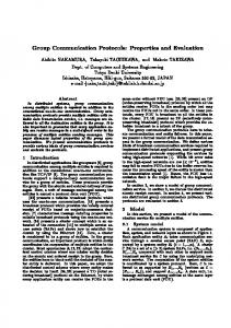
In the following, we consider the modelling of the communication between two stations. In the case of a hierarchical protocol structure in several layers, we consider the specification and validation of one layer, and its relationship to the layers above and below. Fig. 1 shows the component structure of the two stations, from the point of view of the protocol layer implemented in two particular system components, called entity 1 and entity 2. These components use facilities of the component called medium for the exchange of information (at the lowest protocol level, this would be the physical transmission medium between the two stations). In turn, they provide a. communication facility for the components, called user 1 and user 2, of the next higher protocol layer. Therefore, together, the components entity 1, entity 2, and medium can be considered the communication medium to the used by this next higher layer.
I
!
I I user 1 (source)
!
I
I
!
ft user 2 (sink) I
entity 1 (sender)
i
Jl_ medi um
enti ty 2 ] (receiver) I
If
I
Figure 1: Architectural structure of a communication system.
Each component, including the medium, is modelled by a finite state machine. For example, a medium providing unreliable transmission of messages between a sender and receiver component can be modelled by the state diagram of fig. 2. The interface between the components, in our model, are modelled by direct couplings. In the above example, the interface between the sender and the medium would be characterized by the direct coupling ___msenderIImmedium, and the interface between the receiver and the medium by mreceiver II mmedium, and Ereceiver II Emedium (the latter transitions indicating the reception of an erroneous message). The transition type loss and error of the medium would be uncoupled (spontaneous). A similar formalism for the modelling of protocols has been developed independently by Rusbridge and Langsford [3], who also give a characterization of different kinds of simple transmission media.
Figure 2: Finite state model of a simple transmission medium.
G. V. Boehmann / Finite state description of communication protocols 2.3. Protocol validation The validation of protocols specified in terms of interacting finite state components can be automated to a large extend [5,6]. Compared to the approach of specifying protocols in terms of a programming language, where this does not seem feasable, this is an advantage of the finite state approach; although it sometimes seems to be a necessity because of the space explosion of the considered problems. It is difficult to define what protocol validation means. The following points, each describes a certain aspect of the operation of a protocol. Protocol validation can be considered as the analysis of these different aspects, and the comparison of the results obtained with the operational requirements [7]. These principles are the same for protocols and other systems of parallel processes [8]. 2.3.1. Reachability analysis The basis for all subsequent validation aspects is an analysis of the possible transitions of the overall system, the state space of which is the Cartesian product of the state spaces of the interacting components. The reachability analysis yields the transition diagram of the overall system. 2.3.2. Deadlocks A deadlock is characterized by a state of the overall system, reachable from the initial state of the system, for which no further transition is possible. Deadlocks must be avoided, since once the system has arrived in a deadlock state, it is blocked forever. 2.3.3. Liveness A state (or transition) is live if it can be reached from all states of the overall system that are reachable from the initial state. Usually a protocol contains a so-called "home state", or "steady state", which is live and from which all pertinent operations of the protocol can be reached. 2.3.4. Loops Each protocol with a home state contains a loop in the transition diagram of the overall system starting at the home state and leading back to it. Usually, there are other loops necessary for the operation of
363
the protocol. In addition, mostly during the design phase of a new protocol, other loops can possibly be found in the transition diagram. They are undesirable since their execution does not advance tile useful processing of the protocol. Because they could be followed by the system an unlimited number of times, depending on the relative speed of different operations, they have been called "tempo-blockings" [6]. It seems difficult to automatically distinguish between loops that are useful and necessary, and loops that are undesirable. To make this distinction, it is important that the transition diagram of the overall system be comprehensible to the (human) designer. (For the other points of the validation, complete automation seems to be possible). 2.3.5. Self-synchronization and stability A system is self-synchronizing if, started up in any possible state of the overall system, it always returns, after some finite number of transitions, into the normal cycle of operation including the home state. This property is imporant for error recovery in an unreliable environment where, for example, the transmission medium does not always function properly, one station does not follow the prescribed protocol due to a software or hardware bug, or the protocol is not properly initialized. The self-synchronizing property implies protocol stability, because it ensures that the protocol reverts directly to its normal mode of operation after any initial or intermittent perturbation in the synchronization of the two communicating subsystems, introduced for whatever reason. 2.3.6. Characterization o f the operation by action sequences To verify that the actions executed by the protocol correspond to the operations to be performed, it may be useful to characterize the possible action sequences of the overall system by regular expressions [9]. Since the system usually contains loops, the possibility of infite action sequences must be foreseen. This requires an extension [9,10] of the classical formalism of regular expressions. 2.4. Abstraction We consider again the hierarhical aspect of the protocol model shown in figure 1. As explained above,
364
G. V. Bochmann / Finite state description o f communication protocols
the operation of the three components in the broken box is described by an overall transition diagram which is the product of the three interacting components. From the point of view of the next higher protocol layer, i.e. as seen from the components user 1 and user 2, these three components together form a transmission medium. From this point of view the broken box should be described by a finite state diagram containing essentially the transitions that are directly coupled with transitions of the higher level entities user 1 and user 2. Clearly, this diagram may be much simpler than the overall transition diagram of the box, and is therefore an abstraction of the latter. A possible method for obtaining this abstraction is the following: Derive an extended regular expression for the possible action sequences of the protocol (see section 23.6), including as relevant actions only those transitions that are directly coupled with the next higher protocol layer. Then construct a (simple) finite state machine which realizes exactly the action sequences specified by the regular expression. A simple example is given in section 4. 2.5. Limitations o f the finite state approach
The main limitation of the finite state approach to the modelling of protocols is the "state space explosion". A very large number of states are needed to describe a component of a protocol which involves counters or more complex data structures. The number of states is multiplied when the transition diagram of the overall system is constructed (see section 2.3.1). To a certain degree, these problems can be overcome by automated validation tools [5,6]. Another limitation is inherent in the finite state modelling of the transmission medium. This limitation restricts the analysis to situations with only a small number of messages in transit at any given time. In the case of a datagram service or a full duplex link, these conditions are not always satisfied. As an extension to the finite state model described in this paper, regular expressions may be used to model message queues [1] without imposing a limit on the number of messages in transit. The approach using a high-level programming language with assertions on program variables for the specification and validation of protocols seems to be especially useful in cases where the finite state approach encounters problems. Therefore a unified method combining both approaches has been proPOsed [11].
3. The "empty medium" abstraction We call "empty medium abstraction" a simplified view of the overall transition diagram of the protocol, i.e. of the broken box in figure 1, which consists of considering only those states in the product state space of the overall system for which the medium component is empty, i.e. no messages are in transit. This abstraction is particularly useful when the protocol is such that only a small number of messages are in transit at any given time, such as (a) protocols using a two-way alternate mode of transmission (HDX), (b) protocols using a two-way simultaneous mode of transmission (FDX) in a conversational mode, i.e. only a small number of messages are outstanding at any time in each direction. Most initialization protocols are of this nature, and in particular the example treated in section 6. Since the medinm is in the empty state for all states of the protocol considered, the medium component is no longer needed for the description of the protocol in the empty medium abstraction, as indicated in figure 3. Instead, the communicating entities 1 and 2 are directly coupled. The nature of this coupling takes into account the internal structure of the medium. Taking the example of section 2.2. and figure 2, we arrive at a direct coupling between the components sender and receiver which is characterized by the following pairs of coupled transition types: (i) re'sender II mreceiver (correct message transmission, transition path in the medium: i n . m) (ii) ___msender II greceiver (message transmission with error, t~ansition path in the medium: m . error. e)
(iii) ___msenderII /'receiver (message loss, transition path in the medium." m . loss). We note that I denotes the identity transitions, i.e. no transition. In general, the direct coupling between the two
I
r
'[
I
I
entity 1
I
(sender)
k.
a
I-I
I
t-t
H
entity 2
1
J'
(receiver)
-
]I J
Figure 3: Architectural structure of a system with direct coupling between the communicating entities.
365
G. V. Bochmann / Finite state description o f communication protocols
entities is characterized by the set of all paths of transitions within the medium component that lead from the empty state back to this state. Let o = t ~ 1) . t (k2) m "" t(mkn) be the sequence of transition types corresponding to such a path. (In the above example, we may for instance consider o =m__. error. E). Then the direct coupling between the two entities contains all pairs of coupled transition type sequences 01 Jl o2, where o i = t~ iI) • t~ i:) ... t~ in') and o: = t(j ') . t(j 2) ...
t Un') are sequences of transition types of the components entity 1 and entity 2, respectively, such that the transition types of the medium directly coupled with the entity 1 or entity 2 components occur in o in an order compatible with the order of the corresponding transition types in cri and o2. Without loss of generality, we may assume that the sequences ol and o2 begin and end with a transition type coupled to a transition type of o. (In the above example, we obtain ol = m and u2 = E). In general, there may be several pairs o~ II o2 that correspond to one given o, because the oi(i = 1,2) may contain intermediate uncoupled transitions. We note that only a few of all the possible pairs ol I1'o2 are relevant to the communication between the two entities since most of them represent transition sequences which cannot be realized either by entity 1 or entity 2, or both. Examples are given in sections 4 and 6.
D1
A1
-L use
n e w ~
~~new
A!
E,DI
use
Do Receiver Figure 4: State diagram of sender and receiver components. Ao
Sender
the overall system shown in figure 5 (fat transitions only). If we allow for transmission errors, then the following pairs of transition types must be added to the direct coupling: D o[IE, D~[IE,
EIIAo,
EI[A~a
The corresponding transition diagram is shown in figure 5 (fat and thin transitions). If, in addition, we allow for message loss, then the following pairs must be added: OollL
DIHI,
IIIAo,
IliA1
The corresponding transition diagram is shown in fig-
4. A simple example: the alternating bit protocol We consider the alternating bit protocol of Bartlett et al. [12], and use our own notation [11]. The protocol uses the transmission medium usually in a twoway alternate mode. Therefore the empty medium abstraction is suitable for describing the overall transition diagram of the protocol, as explained below.
4.1. Normal operation If we consider a reliable transmission medium with neither transmission errors nor losses, we obtain a direct coupling between the sender and receiver components characterized by the pairs Do II Do,
D~ II D1,
Dt
['
,
~
fl
Ao II A__o, A1 IIA__!.
Based on the transition diagrams of the sender and receiver shown in figure 4 and assuming initialization in the states lo, one obtains the transition diagram of
Figure 5: Transition diagram of the overall system. (Notation: D1 stands forD1 IID1,/~I forD1 IIE, D~I forD1 Ill, etc.)
366
G. 1I. Bochmann / Finite state description of communication protocols
ure 5 (including the dashed transitions). The message loss transitions lead to deadlock states. To recover from these situations, a time-out transition is provided in the sender component, which is supposed to trigger only after a D or A message has been lost, as indicated in figure 5.
4.2. Self-synchronization To check the self-synchronization of the protocol, the overall transition diagram has to be constructed for arbitrary initial states, as shown in figure 6. One sees by inspection that the protocol is self-synchronizing. It is interested to note that, during reliable transmission, a second cycle of operation exists. This cycle (through the states (20, 3~>, etc.) is characterized by simultaneous message transmission through the medium in both directions. In practice this cycle would not be very stable, since message loss could
new
easily occur due to a small mismatch of the processing speeds of the communication components, and would lead back to the normal cycle of operation. To describe the transitions involving simultaneous message transmission in both directions, as shown in figure 6, we have to introduce the following additional pairs of transition types for the direct coupling of the sender and receiver components:
D~Ay II A__g.yDx(correct transmission), DxE [IAyDx, DxAy 11Ay_E, DxE I[ A y E (transmission errors),
Dx 11AyDx, D___xAyl[ A y , Dx l[ A y (loss), D x E I[ Ay, D x II A_!yE (transmission error and loss), where x and y take the values 0 and 1. If the time-out value in the sender is not properly adjusted, or no maximum response time can be established, it is possible that the time-out transition of the sender will occur before the expected response of the receiver actually arrives. This may lead the system from the normal operation cycle onto the second cycle mentioned above. The dotted transitions in figure 6 are those transitions of the overall system which are introduced by assuming no real-time relation between the time-out transition of the sender and the other transitions of the system. The transitions shown are those involving at most one outstanding message in each direction. We note that a very short time-out period may lea~l to cyclic retransmission and several messages in transit (if this is supported by the medium). Although not shown in the figure, these complex transitions do not invalidate the conclusions below.
4.3. Abstraction
new
Figure 6: Complete transition diagram of the overall system (only the part corresponding to the right part of figure 5 is included). Notation: same as in figure 5, and D O IIA0 stands for DoA o IIAoDo, DO IIA0Efor DoE IIAoDo, etc.
From the point of view of the user of the protocol (the next higher protocol layer) only the transitions new and use are of interest. By inspecting figure 6, it is clear that, after proper initialization of the system, the only possible action sequence involving the new and use transitions only is of the form (new. use) °~, i.e. a regular alternation between new. use. new. use ... etc. Therefore the transition diagram of figure 7 is a suitable abstraction of the protocol for the next higher protocol layer. To prove that the transition use actually submits the data that has been obtained during the transition new, it is sufficient to show that between a transition
G. V. Bochmann / Finite state description of commun&ation protocols
367
or exist t] , sl, t'l such that s~ E adj(sl) and sl ~ sl or exist Figure 7: Finite state model of the service provided to the higher level by the alternating bit protocol (abstraction of figure 5).
new and the consecutive transition use of the overall system, there is a correct reception of a D message at the receiver. This is obvious from figure 6. We note that the analysis of action sequences (see section 2.3.6) provides a more general proof method. It is also clear from inspection of figure 6 that the protocol may initially introduce up to two spurious data packets or loose one if it is not properly initialized.
t~ , sy, t; such that s2 E adj(s'l) and s2 -+ sy,
where s i and s~ are states of component i(i = 1,2), t~ lit2 is a pair of directly coupled transition types, and t~ are uncoupled transition types of component i(i = 1,2). This property may be transformed into a set of equations of the form adj(s~ i)) = UFij(adj(sl]))) / where tl
Eft(X)
=
U (S'2 ISl(]') ~ S~i) tl II t2,s2
U U t'2,s2
(s'2Is2 ~ s'2 ^
t2
A S2
p
E X A S2 --~ S 2 }
5. Adjoint states
Considering the protocol model of figure 1, we define for each state sl of the component entity 1 the adjoint states of sa to be all those states s2 of the component entity 2 for which there is a state (Sl, Sm,Sy) of the overail system (where Sm is some state of the medium) which is reachable from the initial state by arbitrarily long paths, i.e. for any given L, there is a path longer then L which leads from the initial state to (Sl, sin, sy). Knowledge of the adjoint states gives information about the relative synchronization between the components entity l and entity 2. When the component entity 1 is in a given state s~, all it knows about the state of entity 2 is that the latter is in one of the adjoint states ofs~ [9]. Clearly, the adjoint states may be obtained from the overall transition diagram of the protocol. In the case of the " e m p t y medium" abstraction or, more generally, in the case of two directly coupled components, the adjoint states satisfy the following property which allows their determination without the construction of the overall transition diagram. Writing adj(sl) for the set of adjoint states of sl, the property may be stated as follows: s~ E adj(s'l)
iff
exist sl, sy, tl II t2 such that s2 E adj(sl), sl ~ sl and t2 t $2 --->S2
s2 ~
X}
U X if exists t' such that s 0)
t' "-~I
and sl i) is the i-th state of component 1. Such a system of equations may be solved by recursive substitution. Using as initial values adj(sli))=s (k) and adj(s~ i)) = 0 for all j v~i yields as the solution, the adjoint states for the case where the components are initialized in states sl i) and s~k), respectively. Using as initial values adj(s~ i)) = (all sy) for all i yields as the solution the adjoint states for the case in which nothing can be assumed about the initialization. Examples are given elsewhere [1].
6. An analysis of the X.25 call set-up and clearing procedures
Some results of an analysis of the X.25 call set-up and clearing procedures have been presented previously [13]. This section gives more details about this analysis, removes some restrictions of the previous work, and shows how the principles outlined in the above sections apply to the analysis of the X.25 procedures. It is also shown that the procedures are stable enough for working in an environment where packets are occasionally lost.
368
G. V. Bochmann / Finite state description o f communication protocols
6.1. The specification of the protocol
6.2. The analysis
The following analysis is based on the protocol defined by figure 8. Contrary to the official X.25 document [14] which uses a single diagram for specifying the procedures, we use two distinct transition diagrams for the two communicating components, one for the DTE and one for the DCE. The advantage of our approach has been pointed out previously [13]. The protocol of figure 8 corresponds to the specifications of X.25, with the following restrictions: a) A clear request and a clear indication may not be sent from the states 1, 2, 5 and 1, 3 respectively. There are two reasons for this restriction: ( i ) i t simplifies the analysis (excluding the repeated clear request and clear indication transitions in the states 6 and 7, respectively, makes the protocol conversational, in the sense of section 3), and (ii) it avoids certain protocol instabilities discussed by Belsnes and Lynning [15]. b) The handling of packets received in the error state is not specified in the standard [14]. On the contrary to our previous work [13], we assume that packets may be received when the component is in the error state. These packets are ignored.
from states 3,4 I
from s t a t e s 1,2,3,4,5
from states 1,2,3,4,5
The protocol occasionally uses the medium in both directions simultaneously. A typical example is given in figure 9 which shows the possible transitions starting in the ready state (1,1 >. The example shows the possibility of call collision, and abnormal system states due to packet loss. The figure also demonstrates the simplification obtained by the use of the "empty medium" abstraction. The main difficulty of the "empty medium" abstraction is to decide which pairs of directly coupled transition types must be included in the analysis for completeness, and which pairs are redundant for the analysis. For example, in order to take care of the possible two-way simultaneous operations, the pairs __m.m' lira . m f o r m E {r, a, £,f} and m' E (i, c, d , f ) must be included in addition to the primitive pairs _m l[ m and m' II m'. But pairs such as /n (1) . m ' ._mm(2) IIm' . m ( O . m(2) need not be included because they are equivalent to the successive execution of the transition pairs__m(1) . m' II m ' . m (1) and m (2) II m (2). The protocol also allows for two consecutive packets to be in transit in one direction. To deal with the possibility of simultaneous packets in the other direction, the transition pairs
from states 2,4,5
OSS DTE DCE Figure 8: State diagram of the X.25 call set-up and clearing procedures. Notation: r: call request; a: call accepted; Q: clear request; f: clear confirmation; i: incoming call; c: call connected; d: clear indication.
Figure 9: Partial transition diagram of the X.25 interface, including states with packets in transit (for instance, ( ~
is
the state where the DTE is in state 2, the DCE in state 1, and a call request is in transit).
369
G. V. Boehmann /Finite state description of communication protocols
m (O . m (2) . m' lira', m (1) • m (2) with m (1) . m (2) = a. l or f . r, and m . m '(1) . m '(2) lira '(1) . m '(~) . m with m '(1) . m ' ( 2 ) = c , d or f . i must be included in the analysis. In order to take care o f possible packet loss, additional pairs of transitions must be considered which are derived from the above by replacing one or more reception transition types by the identity transition (no transition). The annex contains a list of all possible transitions of the overall system in the empty medium abstraction. 6.3. The results
The complete transition diagram of the overalt system is too complex to be shown. The adjoint states are given in table 1 for the following cases: (a) no packet loss (a 1) with initial synchronization (a2) for arbitrary initial states (b) with possible packet loss, and arbitrary initial states (bl) protocol of figure 8 (b2) protocol o f figure 8 with time delay after the transmission o f a clear confirmation packet. The two unexpected adjoint state in case (a2) are due to the two undesired cycles in fig. 10. These potentially infinite cycles may in practice "not persist long given the intrinsic variable time delays and any intelligent processing of the clear by either the DTE or DCE" [16]. These cycles could be completely avoided by introducing, after the transmission of a clear confirmation packet, a time delay longer than the transmission time of the medium, i.e. the X.25 link access procedure [case (b2)]. Table 1 Adjoint states of the DCE for a given state of the DTE. s t a t e o f DTE l 2
3
4
5
6
7
4
5
6
7
l
2
3
l
2
3,6
4
5
6
7,2
1,2, 3,4, 6,7, E
3,4, 5,7
all
1,3, 4,6, 7
all
1,2, 3,4, 7,E
3
3,4, 7,E
3,4, 5,7
I ,3~
7,E
1,2, 3,4, 6,7 E 1,3, 7,E
1,2, 3,4, 5,7, E
4,6, 7,E
E
all 1 ,3~ 4,6, 7
S /
/ f r dlLd f r
/
~: i11Li
~',
Figure 10: Two undesired cycles. We have assumed that a similar time delay is introduced in the error state E before the clear request, or indication respectively, is sent. If this delay is not present, a station in the error state may send the clear before it has received all packets in transit (the other station may have sent two consecutive packets, of which the first has led into the error state). In this way an infinite cycle may occur during which the medium would never be empty, although this is not probable. The adjoint states for the case (a2) indicate that the protocol is stable (except for the cycles mentioned above). This means that after an initial or intermittent perturbation of the synchronization between the two communicating components, introduced for whatever reason, the protocol recovers into its normal mode of operation. The adjoint states for the case (b2) indicate that this is also true when the cycles mentioned above are avoided, and packets may be lost. In this case the DTE knows less about the state of the DCE (for most states of the DTE, there are several adjoint states of the DCE), since after one station has sent a given packet, the other may or may not receive it. It is interesting to note that when the DTE :is in state 3, the DCE is necessarily in the same state. The overall states (2, 3 > and (pairs of adjoint states) are deadlock states. In these states, both components wait {or a response, which will never be sent. This situation can possibly be recovered by retransmission after a time-out period, as in the case of the alternating bit protocol discussed in sec,tion 4. The same time-out mecanism could also recover from the packet loss leading into the states