the CFD modelling of the weld pool fluid dynamics, heat transfer and phase
change, cell-centred Finite Volume. (FV) methods are employed. Alternatively,
novel ...
Second International Conference on CFD in the Minerals and Process Industries CSIRO, Melbourne, Australia 6-8 December 1999
FINITE VOLUME METHODS APPLIED TO THE COMPUTATIONAL MODELLING OF WELDING PHENOMENA Gareth A. TAYLOR, Michael HUGHES, Nadia STRUSEVICH and Koulis PERICLEOUS Centre for Numerical Modelling and Process Analysis, University of Greenwich, London, UK Tel: (44/0)181 331 9768, Fax: (44/0)181 331 8665, E-mail:
[email protected]
ABSTRACT This paper presents the computational modelling of welding phenomena within a versatile numerical framework. The framework embraces models from both the fields of Computational Fluid Dynamics (CFD) and Computational Solid Mechanics (CSM). With regard to the CFD modelling of the weld pool fluid dynamics, heat transfer and phase change, cell-centred Finite Volume (FV) methods are employed. Alternatively, novel vertexbased FV methods are employed with regard to the elastoplastic deformation associated with the CSM. The FV methods are included within an integrated modelling framework, PHYSICA, which can be readily applied to unstructured meshes. The modelling techniques are validated against a variety of reference solutions. NOMENCLATURE p u T
pressure velocity temperature
ρ µ k Cp
density dynamic viscosity conductivity specific heat
∆σ σ Cauchy stress ∆εε Infinitesimal strain ∆d Displacement
INTRODUCTION Essential to the concept of a welding process is the application of a localised heat source in order to minimise the size of the heat affected zone (HAZ) and hence reduce unwanted effects such as distortion and residual stress [8]. Traditionally, when modelling welding phenomena there is a choice, firstly it is possible to focus on the complex fluid and thermo- dynamics local to the weld pool [12,17,20] and secondly it is possible to model the global thermo-mechanical behaviour of the weld structure [5,10]. In the former case only the local geometry of the weld pool and HAZ is considered [12,17,20] and in the latter case a simplified heat source model is employed with heat transfer by conduction only [5,8,10]. Both choices are reasonable as the length scales involved can differ by several orders of magnitude when application areas such as ship construction are considered [7,8]. A variety of simplified heat source models are now frequently employed in the simulation of welding processes, but they are totally reliant on the accuracy of the model parameters which describe the weld pool size
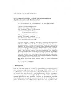
and shape [5,8]. The parameters are obtained from a combination of experimental and calculated data. The scientific and engineering software PHYSICA [14] is a three dimensional numerical modelling framework which can be employed in industrial and environmental applications. The numerical framework consists of both cell-centred and vertex-based FV methods [3,16], which are employed to model problems in CFD and CSM, respectively. These procedures can be readily applied to problems involving complex interactions of physical behaviour over arbitrarily unstructured domains and detailed descriptions of their implementations are available [3,16,19]. For these reasons, the comprehensive modelling of welding phenomena is ideal for demonstrating the versatility of the modelling framework. The ultimate aim of this research is the estimation and verification of the parameters associated with the simplified heat source models in order to achieve consistency between the predictions of the two modelling approaches. It may then be possible to transfer thermal data between analyses of the weld pool and the welded structure via the model parameters. In this paper we will briefly present the modelling of physical phenomena using both approaches. With regard to the thermo-dynamics of the weld pool, surface tension will be accounted for via the inclusion of Marangoni effects [17] and with regard to the thermo-mechanical behaviour of the welded structure, the thermo-elastoplastic distortion of a simple butt weld will be considered [5]. MODEL DESCRIPTIONS The models available in PHYSICA are organised in a modular fashion as illustrated in Figure 1 and the relevant models for the simulation of welding processes are now described. Fluid Dynamics and Heat Transfer
The governing equations for the incompressible fluid flow and heat transfer that can occur in the weld pool are defined as follows; Mass conservation,
∇ ⋅u = 0 , momentum conservation,
ρ
405
∂u + ρ∇ ⋅ (uu ) = −∇p + ∇.µ∇u + S u ∂t
(1)
and heat conservation,
ρC p
∂T + ρ C p ∇.(uT ) = ∇. (k∇T ) + S T . ∂t
The total infinitesimal strain is ∆ε = L ∆d, where ∆d is the incremental displacement. The above solid mechanics capabilities are included within PHYSICA via the EVP module as illustrated in Figure 1 and are coupled with the heat transfer modules in a staggered incremental fashion [16].
(2)
The Darcy and bouyancy source terms are included in equation (1), respectively, as follows;
Su = −
µ u + ρ 0α g (T − T0 ), K
Simplified Heat Source Models
The simplified heat source models that are employed in this paper are as follows; Firstly, the Gaussian heat source over a surface [5]
where K is calculated from the Karman-Kozeny equation [12], ρ0 is the reference density, α is the thermal expansion coefficient, g is the gravity and T0 is the reference temperature. The latent heat source terms are included in equation (2) as follows [12];
ST = −ρ
q(x, z, t ) =
πr2
e
x -3 r
2
e
z + v ( t 0 −t ) -3 r
where fl is the liquid metal fraction and L is the latent heat of fusion. The above models are included with the flow, heat and solidification modules of PHYSICA as illustrated schematically in Figure 1.
q (x, y, z,t ) =
This top surface of the weld pool is subjected to the following flow boundary condition [19,12];
∂s ∇ sT , ∂T
where τ is the flow stress tensor, n is the unit normal of the liquid metal surface, s is the temperature dependent surface tension and is ∇s the surface gradient operator [19]. In this research the surface tension as a gradient of temperature is specified as a model parameter and the curvature effects are neglected as a flat weld pool surface is assumed. The surface tension boundary condition is included within PHYSICA via user access to the sources as illustrated in Figure 1.
6 3 f wQ abc π π
Flow Module
Model Control
e
x − 3 a
EVP Module
General Equation
2
e
y − 3 b
e
z + v(t0 − t) − 3 c
2
,
Solution Control Interpolation
Matrix Solvers
Initialisation
Properties
Sources
Convections
Diffusions
Utility
where L is the differential operator and b is the body force. The incremental stress-strain relationship is defined as follows; ∆σ = D ∆ε e ,
Figure 1: Abstract diagram of PHYSICA.
User Access
File I/O Unit
Geometry Tools
Matrix Tools
Memory Manager
Database Manager
Vector Tools
RESULTS A selection of results obtained from a variety of welding related problems is presented. The various problems employ the models defined in the previous section.
where D is the elasticity matrix. For the deformation of metals the von-Mises yield criterion is employed and the elastic strain is given by ∆ε e = ∆ε − ∆ε vp − ∆ε T ,
Thermo-mechanical Analysis of a Butt Weld
The simple structural configuration of a butt welding process is illustrated in Figure 2. Assuming symmetry along the weld line, only half the structure is modelled. Additionally, if the heat source is moving at a constant velocity then the temperature distribution can be assumed stationary with respect to a moving coordinate system, whose origin coincides with the point of application of the heat source [5,8]. In this manner, it is possible to model a transverse section of the structure as illustrated in Figure 2 using the simplified heat source model described in equation (3).
where ∆εε, ∆εεvp, and ∆εεT are the total, visco-plastic and thermal strain, respectively. The visco-plastic strain rate is given by the Perzyna model [13]
3 s, 2σ eq
where σ eq , σ y, γ, N, and s are the equivalent stress, yield stress, fluidity, strain rate sensitivity parameter and deviatoric stress, respectively. The mathematical operator is defined as follows;
0 when x = x when
(3)
Heat Module
In incremental form, the quasi-static equation of equilibrium is σ)+ b = 0 , LT (∆σ
N
2
System Matrix
Algorithm
Solid Mechanics
1
,
(4) where fw are weighting fractions associated with each ellipsoid, a, b and c are the axes of the ellipses. In both cases x, y and z are fixed coordinates in the weld piece and a constant weld velocity is assumed in the z direction. Both models are also included within PHYSICA via user access to the sources, as illustrated in Figure 1.
Surface Tension Boundary Condition
σ eq d ε vp = γ −1 σy dt
2
where t0 is a time lag factor and Q, r and v are the heat input, characteristic length and velocity weld parameters, respectively. Secondly, the double ellipsoidal heat source over a volume [8]
∂( f l L) − ρ∇.(u f l L ) , ∂t
τ .n = ∇ s s =
3Q
x≤0 . x>0
406
Weld centre-line
Generalised plane strain approximation
WELD LINE
120 TLH Elements Temp. dependent mechanical properties
y
DEFORMED GEOMETRY
x vt
ORIGINAL GEOMETRY X Disp. 0.0
HEAT SOURCE
Y Disp. 0.0
ANALYSED SECTION
Figure 4: Distortion of a butt welded plate. 2.54 mm
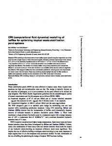
The distortion of the plate after 30 seconds (Mag. ×50) is illustrated in Figure 4. The distortion differs from that of the original analysis. This was to be expected as the original analysis included plastic strain removal due to melting [5] and as a model for the removal of plastic strains is not available within PHYSICA at present it was not possible to perform identical analyses. Contours of the residual effective plastic strain in the HAZ are illustrated in Figure 5. As expected, the plastic strain intensity increases close to the application of the heat source and the change of intensity can be associated with the extent of the weld pool.
150 mm
z
Figure 2: Schematic diagram of butt welding. With regard to the solid mechanics, a generalised plain strain boundary condition is applied in the z direction and an ideal elasto-plastic material behaviour is associated with the plate. The welding parameters are equivalent to those of Friedman [5]; heat input Q = 703 W, characteristic length of heat flux r = 5.08 mm and weld velocity v = 2.12 mm/s. These values were originally chosen to illustrate the thermo-mechanical response of a full penetration weld. The thermo-mechanical analysis was performed in a staggered incremental fashion. Equivalent spatial and temporal discretisation was employed to that of the original analysis [5]. The temperature independent material properties associated with the heat transfer analysis are described in Figure 3. The temperature dependent material properties for the thermal and mechanical analyses are equivalent to those used in the original analysis [5].
E
I H
Liquidus 1690 K Solidus 1630 K Latent heat of fusion 309 kJ/kg
x=0
1.5 Temp. K
x=2.5mm x=5.0mm
1 .75 .5
32.0mm 0
5
10 Time Sec.
15
20
25
30
F
Contour range A = 0.6% to J = 1.8%
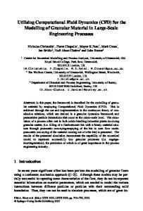
Results obtained using the simple heat source models described by equations (3) and (4) are illustrated in Figure 6. When they were proposed, both these models were originally compared against the experimental data of Christensen et al. [2]. The temperature profiles illustrated in Figure 6 are plotted perpendicular to the direction of the weld line, 11.5 seconds after the heat source has passed. With regard to the heat sources, the same local coordinate system is employed as in the previous analysis. The results obtained from PHYSICA are in close agreement with the original results obtained for both models and illustrate again the closer agreement of the ellipsoidal model proposed by Goldak et al. [8] with regard to the experimental results. The lack of accuracy of the surface model employed by Krutz and Segerlind [11] has been demonstrated with regard to certain welding applications, ie. deep penetration electron or laser beam welding [8], where the digging action of the heat source is not captured. It is important to note that both models require a modified value of conductivity in the weld pool during the liquid phase [11,8]. This is to account for the possible transfer of heat by convection. The accuracy of the numerical analyses employing these models is very sensitive to the conductivity and therefore a thorough understanding of
Conductivity and specific heat are temp. dependent
1.25
.25
A
Comparison of Simplified Heat Source Models
2 1.75
B
Figure 5: Residual plastic strains in the HAZ.
Iconel alloy 600 (NiCrFE)
2.25
C
G
Extent of weld pool
Y * 1.0E3 2.75 2.5
D
H J
35
Figure 3: Surface temperatures of welded plates. The temperature profiles at locations on the upper surface of the plate are illustrated in Figure 3 and are in reasonable agreement with the results obtained by Friedman [5]. The results can differ on equivalent meshes because a cell-centred FV method is employed within PHYSICA with regard to the heat transfer [3], where as a vertex-based FE method was employed in the original analysis [5]. Therefore, in order to perform a comparison the temperatures have to be extrapolated from the cell centres to the vertices, which can lead to discrepencies.
407
the weld pool thermodynamics is required in order to modify the conductivity values correctly. The ultimate aims of this research are to determine heat source model parameters and modified values of conductivity that are consistent with the predicted thermodynamics of particular weld pools.
0.03
0.02
Ux (m/s) 0.01
Analytical Numerical FV
2500
0.00 2000
-0.01 0.00
1500
Temp.
0.05
0.10
0.15
0.20
0.25
0.30
0.35
0.40
0.30
0.35
0.40
Distance (m)
(deg K) Ellipsoidal Surface Christensen (Experimental)
1000
Figure 8: X component velocity profile
500
0
6.E-03
0.000
0.005
0.010
0.015
0.020
0.025
0.030
0.035
0.040
Distance (m)
Figure 6: Temperature profiles after 11.5 seconds.
4.E-03
Uy (m/s)
Marangoni Convection in Weld Pools
Analytical Numerical FV
Two problems will be considered. The first case is the motion of a liquid resulting from a free surface, where the surface tension is quadratically dependent on temperature [9]. The second case is the inclusion of Marangoni effects in the axisymmetric modelling of weld pools [17]. In both cases reference solutions are available.
2.E-03
0.E+00 0.00
X=0
0.20
0.25
As illustrated the results are in good agreement with the analytical solution [9]. Case 2
The stationary and steady state fusion of an aluminium plate by a heat source defined over a surface is considered. The model for the steady state heat source distribution is obtained from equation (3) as follows;
q (x ) =
3Q πr
e
x - 3 r
2
.
An axisymmetric approximation is assumed, and convective and radiative heat loss boundary conditions applied on remainder of the surface, x > r . To enable a localised analysis, it is assumed that the boundary conditions away from the axis and surface can be derived from the analytical solution for an equivalent point heat source [15].
∂u ∂T ∂s ∂T = 0, µρ X = = β(T − T0 ) ∂Y ∂Y ∂X ∂X
Y
0.15
Figure 9: Y component velocity profile
The thermo-capillary motion of an idealised liquid with surface tension as a quadratic function of temperature is considered. The boundary conditions required for the thermo-capillary analysis are illustrated in Figure 7. In this analysis a 10 by 0.4 aspect ratio is employed with regard to the geometry. Thus permitting the application of a symmetry condition at a finite distance from the region of interest. The region of interest is defined by the cross section x-s, which is close to the boundary T = T0 as illustrated in Figure 7.
Symmetry
x-s (X = .625m)
0.10
Distance (m)
Case 1
T = T0
0.05
X = 10
T = T0 + aX , u X = uY = 0 X
Marangoni Affected Weld Pool ds/dT = -0.35E-3
Figure 7: Thermo-capillary boundary conditions
1200 900 652 (liquidus)
The constants β and a, define the quadratic relationship of surface tension s to temperature T, and the linear variation of temperature and spatial coordinate X, respectively. The resultant velocity component profiles are plotted in Figures 8 and 9, along the cross section x-s illustrated in Figure 7.
582 (solidus)
0.22 m/s
5mm .................
Figure 10a: Negative: Temperature and flow fields
408
FURTHER RESEARCH 1200
Currently, there are a number of methods for modelling welding processes depending upon the reference frame associated with the heat source. Essentially, the methods are Eulerian, where the heat source is stationary [1,7], or Lagrangian, where the heat source is moving [18,4]. The methods employed in this paper for welding processes involving a moving heat source are a variation of the Lagrangian approach, such that the heat source model is transformed as a function of time. This approach is reasonably accurate for simplified heat sources moving with a constant velocity [6], but it is not suitable when modelling the fluid dynamics of a weld pool associated with a moving heat source. Therefore, further research will involve the development of Eulerian techniques within PHYSICA, which will facilitate the localised modelling of the fluid dynamics associated with a moving weld pool. Additional further research will involve the inclusion of Lorentz effects, which are necessary for modelling arc welding processes, where electro-magnetic fields can exist and interact with the fluid dynamics of the weld pool. With regard to global thermo-mechanical analyses of a welded structure, further research will involve the three dimensional application of simplified heat sources associated with a Lagrangian reference frame [4,18]. It should be noted that thermo-mechanical analyses have been performed using Eulerian and Lagrangian frames of reference for the heat source and mechanical behaviour, respectively [7]. However, this approach is not generally suitable for the welding of large structures, particularly when welding sequences are involved. This is because the local mechanical constraints do not necessarily reflect the global mechanical behaviour. For these reasons most thermo-mechanical analyses of the welding of large structures involve the former technique [4,18].
900 652
Figure 10b: Negative: Temperature and flow fields [17] The results from the numerical analysis are illustrated in Figures 10a and 11a with regard to a negative and positive surface tension gradient, -.35e10-3 and +.1e10-3 kg/(s2K) respectively. The different gradient values represent types of alloy and illustrate the different alloy related Marangoni effects on the velocity and temperature fields. The temperature fields are contoured in degrees Celsius and as illustrated by Figure 10a the shape of the weld pool is flatter for the negative gradient case. The change in weld pool shape is related to the different flow patterns that occur in each weld pool, as illustrated in Figures 10a and 11a. For the negative or positive gradient case the predominant flow is away from or towards the heat source, respectively. In this way the convective heat transport is directed towards or away from the axis, resulting in either a deeper or flatter weld pool shape, respectively. Marangoni Affected Weld Pool ds/dT = +0.1E-3 1200 582 (solidus)
900 652 (liquidus) 0.20
5mm .................
CONCLUSION In this paper we have demonstrated the versatility of PHYSICA with regard to the comprehensive modelling of welding phenomena and investigated the two standard approaches to the modelling of welding. Based on the results obtained, it is now possible to draw a number of conclusions with regard to our original aims. Focussing on the modelling of the distortion that can occur in the welding of large structures [18], when a simplified heat source model is employed, a number of required parameters must be determined accurately. These parameters mainly depend upon the welding process employed and the material that is being welded. For laser or electron beam welding a digging phenomena is observed with regard to the weld pool [8,18]. This digging effect has been modelled successfully using simplified heat source models. This has been achieved either by using a conical heat source model with a modified isotropic conductivity for the liquid region [6] or a surface model with a modified orthotropic conductivity in the liquid region [18]. The accuracy of both methods is therefore dependent upon the modifications to the conductivity in the liquid region and this dependency was observed for the simplified heat source models studied in this paper. Indeed, it is possible to view the modification of the conductivity in the liquid region as an additional data fitting exercise when using simplified heat source models [6]. However, it is important to note that the modifications to the liquid conductivity are intended to
Figure 11a: Positive: Temperature and flow fields
1200
900 652
Figure 11b: Positive: Temperature and flow fields [17] The results are in good agreement with those obtained by Tsai and Kou [17], which are represented in Figures 10b and 11b. The results for the negative case are in general agreement with regard to weld pool shape, temperature field and flow field as illustrated in Figures 10a and 10b. Additionally, the results for the positive case are also generally in good agreement as illustrated in Figures 11a and 11b. Although it should be noted that in the positive case PHYSICA predicts a slightly deeper weld pool shape.
409
14. PHYSICA, MPS Ltd., 5 The Priors, Harriots Lane, Ashtead, Surrey, UK. 15. ROSENTHAL, D., (1946), “The Theory of Moving Sources of Heat and Its Application to Metal Treatments.”, Trans. ASME, 68-11, 849866. 16. TAYLOR, G. A, (1996), “A vertex based discretisation scheme applied to material nonlinearity within a multi-physics finite volume framework.”, PhD thesis, The University of Greenwich. 17. TSAI, M. C. and SINDOU KOU, (1989), “Marangoni convection in weld pools with a free surface”, Int. J. Num. Methods Engrg., 9, 15031516. 18. VOSS, O., DECKER, I. and WOHLFAHRT, H., (1998), “Consideration of microstructural transformations in the calculation of residual stresses and distortion of larger weldments.”, In H. Cerjak, Editor, Mathematical Modelling of Welding Phenomena 4, 584-596. 19. WHEELER, D., BAILEY, C. and CROSS, M., (1999), “Numerical modelling and Validation of Marangoni and Surface Tension Phenomena Using the Finite Volume Method”, Int. J. Num. Methods in Fluids, 212-B, accepted for publication. 20. ZACHARIA T., DAVID, S. A., VITEK J. M. and KRAUS H. G., (1991), “Computational modelling of stationary gas-tungsten-arc weld pools and comparison to stainless steel 304 experimental results”, Met. Trans B, 22B, 243257.
account for the redistribution of heat by convection. Therefore, a future aim of this research is to establish modified values of conductivity and associated model parameters that are consistent with an analysis of the fluid dynamics of the weld pool. REFERENCES 1.
2.
3.
4.
5.
6.
7.
8.
9.
10.
11. 12.
13.
CHEN, X., BECKER, M., and MEEKISHO, L., (1998), “Welding analysis in moving coordinates.”, In H. Cerjak, Editor, Mathematical Modelling of Welding Phenomena 4, 396-410. CHRISTENSEN, N., DAVIES, V. DE L. and GJERMUNDSEN, K., (1965), “Distribution of temperatures in arc welding”, British Welding Journal, 12, 54-75. CROFT, T. N., (1998), “Unstructured mesh – finite volume algorithms for swirling, turbulent, reacting flows.”, PhD thesis, The University of Greenwich. FENG, Z., CHENG, W. and CHEN, Y., (1998), “Development of new modeling procedures for 3D welding residual stress and distortion assessment.”, Cooperative Research Program, SR9818. FRIEDMAN, E., (1975), “Thermomechanical Analysis of the Welding Process Using the Finite Element Method”, Journal of Pressure Vessel Technology, Trans. ASME, 97, 206-213. GOLDAK, J., BIBBY, M., MOORE, J., HOUSE, R. and PATEL B., (1986), “Computer Modelling of Heat Flow in Welds.”, Met. Trans. B, 17B, 587-600. GOLDAK, J., BREIGUINE, V. and DAI, N., (1995), “Computational Weld Mechanics: A Progress Report on Ten Grand Challenges”, In H. B. Smartt, J. A. Johnson and S. A. David, editors, Trends in Welding Research – IV, 5-11. GOLDAK, J., CHAKRAVARTI, A. and BIBBY, M., (1984), “A New Finite Element Model for Welding Heat Sources”, Met. Trans. B, 15B, 299-305. GUPALO, Y. P. and RYAZANTSEV, Y. S., (1989), “Thermocapillary motion of a liquid with a free surface with nonlinear dependence of the surface tension on the temperature”, Fluid Dynamics, (English translation), 23:5, 752-757. KISELEV, S. N., KISELEV, A. S., KURKIN, A. S., ALADINSKII, V. V. and MAKHANEV, V. O., (1999), “Current Aspects of Computer Modelling Thermal and Deformation Stresses and Structure Formation in Welding and Related Technologies”, Welding International , 13-4, 314-322. KRUTZ, G. W. and SEGERLIND, L. J., (1978), “Finite element analysis of weld structures”, Welding Research Supplement, 57, 211s-216s. PERICLEOUS, K. and BAILEY, C., (1995), “Study of Marangoni phenomena in laser-melted pools”. In J. Campbell and M. Cross, editors, Modeling of Casting, Welding and Advanced Solidification Processes - VII, 91-100. PERZYNA, P., (1966), “Fundamental problems in visco-plasticity.”, Advan. Appl. Mech., 9, 243377.
410