Wenjuan Gong, Michael Sapienza, and Fabio Cuzzolin. Oxford Brookes
University, UK. {wgong,michael.sapienza-2011,fabio.cuzzolin}@brookes.ac.uk.
Abstract ...
Fisher Tensor Decomposition for Unconstrained Gait Recognition Wenjuan Gong, Michael Sapienza, and Fabio Cuzzolin Oxford Brookes University, UK {wgong,michael.sapienza-2011,fabio.cuzzolin}@brookes.ac.uk
Abstract. This paper proposes a simplified Tucker decomposition of a tensor model for gait recognition from dense local spatiotemporal (S/T) features extracted from gait video sequences. Unlike silhouettes, local S/T features have displayed state-of-art performances on challenging action recognition testbeds, and have the potential to push gait ID towards real-world deployment. We adopt a Fisher representation of S/T features, rearranged as tensors. These tensors still contain redundant information, and are projected onto a lower dimensional space with tensor decomposition. The dimensions of the reduced tensor space can be automatically selected by keeping a proportion of the energy of the original tensor. Gait features can then be extracted from the reduced “core” tensor, and ranked according to how relevant each feature is for classification. We validate our method on the benchmark USF/INIST gait data set, showing performances in line with the best reported results.
1
Introduction
Gait recognition has been extensively studied as a behavioral biometric technique. Identity recognition from gait is non-invasive, can be measured at a distance, is difficult to disguise or occlude, can be identified even in low-resolution images, and is non-cooperative in nature. In opposition, most other biometrics, such as finger-prints [2], faces [3], hand geometry [4], irises [5] and voices [6] can be captured only with contact or within a close distance. However, its adoption in real-world scenarios is limited by the influence of a large number of nuisance or “covariate” factors [16] which affect appearance and dynamics of the gait, such as viewpoint changes, variations in clothing and footwear, changing floor types, different carrying conditions and so on. Thus, how to extract robust features and how to represent them in a form that is suited for gait recognition constitute challenging problems. Traditional approaches to gait recognition make use of extracted human body silhouettes as input. Silhouettes allow us to represent a human blob via a concise descriptor, which can be later analyzed in the frequency domain to detect gait cycles. Typically, either a template matching step [7] or statistical modeling (for example, by estimating a hidden Markov model from the silhouette sequence [17]) follow. The problem is that silhouette extraction requires robust
2
Wenjuan Gong, Michael Sapienza, and Fabio Cuzzolin
background subtraction, an extremely difficult task to achieve in challenging real-world environments characterised by strong variations. State-of-the-art approaches in action recognition from videos, on the other hand, rely on the selection of local features from the spatiotemporal (S/T) volume associated with each video [18, 19]. This choice of features has helped progress towards recognition in unconstrained environments with cluttered backgrounds [1]. Different local feature descriptors can capture different video attributes. For example, Histograms of Oriented Gradients (HOG) features are designed to capture the appearance of frames, while Histograms of Optical Flow (HOF) and Motion Boundary Histograms (MBH) encode local motions. The challenge is how to represent this array of various local features in order to retain the structure of their interaction. In many problems, data come naturally in the form of higher-dimensional, multi-way arrays or “tensors”, rather than one-dimensional vectors. This is indeed the case for video analysis, in which image sequences are inherently order-3 tensors which depends on row, column and time frame indices. Tensor decompositions of high dimensional arrays into subspaces representing the various covariate factors have been shown to facilitate data analysis, for instance in face recognition [20]. Indeed, tensor decompositions are intensively studied [9, 8, 10, 11]. Consequently, in this work we adopt tensors for representing the multiple local features extracted from input videos. In this way, tensor decomposition methods can be applied to retain the structure of the interaction among the various features, while performing at the same time dimensionality deduction. Feature Selection
Training Tensor
×2
~ ~
×3
vectorize
X
G
B
A
Train
G SVM
T
Test Tensor
G’ = X’×2A ×3B
T
vectorize
Test
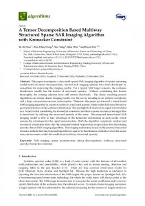
X’ G’ Fig. 1. A bird’s eye view of the proposed tensor classification framework.
Figure 1 shows the overall pipeline of our gait recognition method. Rather than using silhouettes as in most gait recognition algorithms, we introduce a state-of-art descriptor, Fisher vectors [21] of dense trajectory features [19], to encode video sequences. This descriptor has achieved state-of-art performance on action recognition problems [12], and has the potential to allow gait identification in realistic, unconstrained environments. In addition, instead of representing each video as a vector of concatenated fea-
Fisher Tensor Decomposition for Unconstrained Gait Recognition
3
tures, we rearrange them into order-2 Fisher tensors (matrices) so that the structure of the interaction among the various feature types and their components can be learned and exploited to generate the final feature descriptors for recognition. The training data is arranged into an order-3 input tensor X with one dimension for training sample index, one for the different local feature types, and one indexing the components of each feature vector. In training, we employ a Tucker-2 decomposition on the training tensor X resulting into a set of training bases A and B (Figure 1-top). In testing (Figure 1-bottom) these bases are used to project the Fisher matrix X ′ of a new video to a lower-dimensional tensor space, whose core tensor G ′ is vectorised to form a video feature vector and classified via linear SVM. The proposed method is validated on the benchmark USF database in the original experimental settings, which analyse the influence of nuisance factors such as change of viewpoint, change of floor types and so on, delivering results comparable and at times superior to the best reported results.
2
Fisher Tensor Representation of Local S/T Features
To push towards gait recognition “in the wild”, we first extract dense local features from the spatiotemporal (S/T) volumes associated with the video sequences. A vocabulary of the most representative local features is learned, so that each video sequence is represented as a distribution on the vocabulary. While in the traditional bag-of-features pipeline this distribution is a histogram, we adopt a Fisher vector representation, which retains more information via soft assignments to visual words.
2.1
Dense Trajectories
For our experiments we picked Dense Trajectories, since they demonstrated excellent performance in unconstrained action recognition [19]. Dense Trajectory features are formed by the sequence of displacement vectors in an optical flow field, together with the HoG-HoF [18] and the motion boundary histogram (MBH) descriptors computed over a local neighborhood along the trajectory. We keep the default parameters: features are computed in video blocks of size 32 × 32 pixels for 15 frames, with a dense sampling step size of 5 pixels [19]. We build a visual word vocabulary by sampling features from the training set and clustering them by k-means. The k-means algorithm was initialized 8-times and the configuration with the lowest error selected. Each trajectory is represented by a vector of dimension 426, composed of five sections: trajectory (30), HOG (96), HOF (108), MBHx (96) and MBHy (96). A video sequence containing 200 dense trajectories would be represented by a vector of 85200 components. To get a more concise representation we apply PCA as in [12], and retain 24 dimensions for each of the five feature components.
4
2.2
Wenjuan Gong, Michael Sapienza, and Fabio Cuzzolin
From Bag of Words to Fisher Tensors
In the standard Bag of Words (BoW) setup local feature descriptors from still images or video sequences (in our case, dense trajectories of decreased dimensions via PCA) are clustered, so that cluster centers compose a vocabulary. Euclidean distances between vocabulary words and all local descriptors are measured, and local features are assigned to the closest one. Finally, an image or video is represented as a histogram by counting the occurrences of all vocabulary words. There is evidence in image classification and retrieval, however, that a Fisher representation [21] outperforms BoW histograms. Instead of creating a visual vocabulary by clustering the feature space by k-means, as in the BoW approach, we assume that features are distributed according to a parametric Gaussian Mixture Model (GMM). A Fisher vector is formed by soft assignment of each feature point to each Gaussian in the visual vocabulary. Here, we choose a dictionary size of 128 for each of the five feature components. The overall Fisher vector representation for each video sequence has then size 24 (reduced dimension of each descriptor type) ∗5 (number of different types of local features) ∗128. Crucially, we rearrange each video Fisher vector into a matrix (order-2 tensor) of size 128 (number of visual words) × (24 ∗ 5). A training set of videos is then mapped to a training set of Fisher matrices. By stacking those matrices along a third dimension (indexed by the video numbering) we represent the training set as an order-3 tensor X (Figure 1). 2.3
Why tensors of local features
In general, an order-N tensor or multi-way array X = {xi1 ,i2 ,··· ,iN , ij = 1, ..., Ij } is a collection of scalars indexed by an arbitrary number N of indices. Each index expresses a “mode” of variation of the data. The mode-s matricizing of Q an order-N tensor X generates a matrix X(n) of size In × m6=n Im , obtained by concatenating all the vectors of length Im associated with a fixed value of all the indices m 6= n. Now, local features extracted from images or video sequences come with information on their location and co-occurrence, which is simply destroyed when representing them as long, concatenated vectors. In situations affected by a number of covariate factors, instead, tensors can be arranged in a way such that each dimension correspond to one of the relevant factors. In gait recognition, for example, tensors could be formed with separate modes for person identity, camera viewpoint setting, clothing conditions, and so on. Tensor analysis is then able to decompose the input tensor into a collection of subspaces, each describing the modes of variations of each specific factor [9]. In particular, when only two such factors are present, bilinear models [13, 14] are able to represent the input observations as a mixture of a “style” (nuisance) and a “content” (the label to classify) variable. Unfortunately, this type of analysis performs well only when the training set contains a rich collection of different cases (possible values) for each factor, a fact that hinders its application.
Fisher Tensor Decomposition for Unconstrained Gait Recognition
5
By arranging the training tensor with one mode for sample index, one for feature type, and one for feature vector component as proposed in Section 2.2, instead, we tailor our tensorial framework to be suitable for representing multiple features captured under a few cases or even only one case of the varying nuisance factors (in the experiments of Section 4, the training data only have one specific value for each nuisance factor). In Section 3 we show how to apply a Tucker-2 decomposition to extract and classify the structure of the interaction between local features from test videos.
3
Tucker Dimensionality Reduction of Fisher Tensors
Tensor decomposition approaches [9] allow to decompose a tensor into its N constituent modes. Different tensor decomposition models have been proposed: CANDECOMP/PARAFAC (CP) [22], Higher-Order Singular Value Decomposition or HOSVD [23], Nonnegative Tensor Factorization (NTF) [24] and the Tucker model [9]. PARAFAC, HOSVD and NTF can all be seen as special cases of Tucker decompositions under different conditions of orthogonality diagonality or non-negativity [15]. Since the CP decomposition imposes the same dimension for the decomposed core tensor, while we obviously need to automatically tailor the dimensionality of each mode based on the training data, we choose here a Tucker (specifically a Tucker-2) decomposition. The details and the advantages of this decomposition method are explained in the following subsections. 3.1
Estimating a Tucker-2 Decomposition
In this paper, instead of carrying out a standard Tucker decomposition, we seek a “Tucker-2” decomposition of the order-3 training tensor X (of dimensions I1 × I2 × I3 ) into a a core tensor G and two basis factors: X ≈ G ×2 A ×3 B,
(1)
where ×n is the n-mode product of a tensor Q = {qi1 ,i2 ,...,in ,...,iN } by a matrix P = [pjn ,in ], X (2) qi1 ,i2 ,...,in ,...,iN ∗ pjn ,in , (Q ×n P )i1 ,i2 ,...,jn ,...,iN = in
and the matrices A (of size I2 × L) and B (I3 × M ) collect the basis vectors spanning two separate subspaces for the two modes of the input tensor. Such a decomposition allows us to separate the influence of the two factors (feature component and feature type) on the observed videos, while the intrinsic structure of the interaction between feature components and feature types is retained by G. At the same time, dimensionality reduction can be performed by setting for the core tensor G mode dimensions smaller than the input tensor’s. Compared to the classical Tucker-3 decomposition, the Tucker-2 decomposition (1) is more efficient during training and optimization, due to its fewer model parameters.
6
Wenjuan Gong, Michael Sapienza, and Fabio Cuzzolin
Given an input tensor X we can estimate a Tucker-2 model by minimising the Frobenius norm [23] of the difference between the input tensor and its Tucker approximation: kX − G ×2 A ×3 Bk2F . (3) A common approach to the minimisation of Equation (3) is based on Alternating Least Squares. Without loss of expressive power, we can require the decomposed matrices A and B to be orthonormal. Singular Value Decomposition (SVD) is performed on the mode-n matricised versions of the tensor multiplied by all other factor matrices except the n-th factor matrix. This is to get the eigenvectors of the n-th factor matrix given the values of all other factor matrices, and the first several dimensions representing most variations of the original tensor are extracted. This results in the following updates: T
U (2) S (2) V (2) = X(2) (E ⊗ B), (2)
T
U (3) S (3) V (3) = X(3) (E ⊗ A),
(4)
(3)
where At+1 ← Ucol=1,...,L and B t+1 ← Ucol=1,...,M are the new basis matrices at iteration t + 1 and E is an identity matrix of size I1 × I1 . At each iteration the core tensor G is estimated via: G ← X ×2 AT ×3 B T .
(5)
In a following step, estimated tensor Xˆ is updated as Xˆ = G ×2 A ×3 B. Then the difference between the input tensor X and the Tucker-2 approximation Xˆ is calculated (as in Equation(3)) and compared to a pre-defined threshold. That is, the algorithm alternates between Equation (4) and Equation (5) until a certain iteration number is reached or the change in the error (3) to minimise is below a set threshold. This procedure is similar as Higher-Order Orthogonal Iteration (HOOI) algorithm in [9]. 3.2
Feature Selection and Classification
Once the basis matrices A and B are learned from the proposed Tucker-2 decomposition of the training tensor, we can use them to project any test order-2 tensor (i.e., the Fisher matrix extracted from a test video) to a lower dimensional subspace. This can be done via Equation (5): the result is a core tensor of reduced dimensionality. The latter dimensionality, for any given mode, can be automatically set by selecting the number of dominant eigenvalues of the covariance of the mode-n matricised version X(n) of the training tensor X (as in [15]): T = U ΛU T , X(n) X(n)
(6)
where Λ = diag(λ1 , λ2 , . . . , λIn ) and λ1 ≥ λ2 ≥ · · · ≥ λIn are eigenvalues. The suitable dimension is such that all variations above a threshold θ are retained: Pm j=1 λj > θ. (7) arg min PIN m j=1 λj
Fisher Tensor Decomposition for Unconstrained Gait Recognition
7
For tensors of order 3, the resulting core tensor G is rearranged into a (feature) vector g of length U = I1 ∗ L ∗ M . Given a training set of T videos distributed among C different classes (in the tests of Section 4, IDs), with Tc videos per class c = 1, ..., C the components u of the vectorised core tensor are ranked according to their Fisher scores [15]: PC
c=1 ϕ(u) = P T
Kc (g¯u c − g¯u )2
t t=1 (gu
− g¯u ct )2
,
u = 1, . . . , U,
g¯u c =
1 X t g , Tc t∈c u
g¯u =
T 1X t g , T t=1 u
where gut is the u-th component of the vectorised core tensor g t for video t = 1, ..., T , ct denotes the class (ID) of t-th training video, g¯u c is the average u-th component for video of class c, g¯u is the mean of the u-th component over all training videos and Kc is the number of training samples in class c. All components u whose score ϕ(u) is above a threshold τ are retained. After all features (components of g) are ranked based on the Fisher scores, those with top scores are chosen for classification. For the latter we adopt a linear Support Vector Machine (SVM), due to its consistent performances in image, scene and action classification problems. We use a standard implementation of linear SVM with cost set to 100 (as in [12]), a factor which has shown not to be consequential for classification performance.
4
Performance on the USF database
We validated the proposed approach on the public USF/INIST benchmark data set, arguably the most challenging gait ID testbed to date. This data set contains a large collection of videos, a standard set of twelve experiments and a baseline algorithm. It consists of 1870 sequences from 122 subjects and 5 covariates: viewpoint (R-right or L-left), shoe type (A or B), walking surface (G-grass or Cconcrete), carrying or not carrying a briefcase (B or NB), and temporal difference (M or N, as sequences are shot in two different times of the year). The training set is the same for all experiments. Each experiment concerns walking gaits from 122 individuals, and considers a specific combination of the five covariates. The experimental setting is explained in detailed in [7]. Table 1 compares the performance on the original USF experiments of the following approaches: 1- the USF baseline algorithm; 2- the state of the art MMFA approach; 3- direct SVM classification of Fisher vectors computed from Dense Trajectory features (without tensor decomposition), which has been successfully applied to action recognition from videos [12] (FV); 4- classification of Fisher matrices as order-3 tensors after Tucker-2 dimensionality reduction (by retaining the 0.98 percent of the spectral energy of input tensor) and discriminative feature selection (FVTD). Recognition accuracies are compared using two criteria: Rank 1 (“R1”) and Rank 5 (“R5”). Under Rank 1, the recognition is considered to be correct when the first ranking is the same as the ground truth label. Rank 5 means that the recognition is considered to be correct when the top five ranking contain the ground truth label. From Table 1, we can see that Fisher vector SVM classi-
8
Wenjuan Gong, Michael Sapienza, and Fabio Cuzzolin Exp. Difference Baseline MMFA FV FVTD R1 R5 R1 R5 R1 R5 R1 R5 A B C D E F G H I J K L Avg.
V S S, V F F, S F, V F, S, V B B, S B, V T, S, C F, T, S, C
73 78 48 32 22 17 17 61 57 36 3 3 41.0
88 93 78 66 55 42 38 85 78 62 12 15 64.5
89 94 80 44 47 25 33 85 83 60 27 21 59.9
98 98 94 76 76 57 60 95 93 84 48 39 79.9
97 81 78 14 12 25 17 93 90 81 0 9 55.7
100 91 91 50 45 50 47 97 93 97 24 27 73.2
98 80 78 21 17 25 15 94 90 83 3 9 57.2
100 93 91 45 45 46 47 97 93 98 21 21 72.0
Table 1. Comparison of gait recognition accuracies (in %) for the baseline method, the state-of-art MMFA approach, Fisher vector (FV) SVM classification and Fisher vector after tensor decomposition (FVTD). “R1” and “R5” denote Rank 1 and Rank 5 respectively.
fication (FV) outperforms the baseline algorithm by 14.7% for Rank 1 and by 8.7% for Rank 5. FVTD, classification of Fisher matrices after tensor projection and feature selection, has an even better Rank 1 performance, improving on the baseline approach by 16.2% (and by 7.5% for Rank 5). By classifying the intrinsic structure of the interaction among the different features, FVTD outperforms FV by 1.5% in Rank 1 evaluation. In some of the USF experiments covariate factors strongly affect the extracted silhouettes: for instance, when varying carrying conditions the silhouettes tend to be very different with or without the suitcase. In these experiments, FV and FVTD tend to outperform even the state-of-art method MMFA. E.g., in experiment H FVTD outperforms MMFA by 9% in Rank 1. Although the average recognition accuracies of MMFA are higher than those of both FV and FVTD, we should keep in mind that FV and FVTD can be applied to video sequences captured in unconstrained environments and surveillance videos, while MMFA (which depends on silhouette extraction) arguably cannot. In a sense, even the USF database in not challenging enough to discriminate between silhouette-based approaches and our proposal based on local S/T features. By comparing FV and FVTD we can observe that FVTD tends to outperform or at least have equal performances as FV in eleven experiments out of twelve. This suggests that, when data are naturally presented in tensor form, tensorial dimensionality reduction delivers better recognition accuracy than the original features, by retaining the most discriminative information and discarding noise. Two parameters of the feature selection procedure (Section 3.2) need to be empirically determined: the threshold θ in Equation (7) and the threshold τ for the ranked scores (8). In these experiments we set θ to 0.98 (as in [15]) and τ to 0.5 × τ , where τ is the average score. The latter does not have as much impact on performance as θ.
Fisher Tensor Decomposition for Unconstrained Gait Recognition
5
9
Conclusions and Future Work
In this paper we proposed an effective method for gait recognition from dense local features in unconstrained video sequences. Results on the benchmark USF database show that applying tensorial dimensionality reduction to Fisher vectors in tensor form yields a better accuracy, helping to factor out the influence of the many nuisances and keep the interacting structures among different feature dimensions and feature types. The dimensions of the reduced tensor are automatically set by analysing the input tensor: however, from our tests there does not seem to be a direct relation between the resulting dimensions and recognition accuracies. Better criteria for discriminating feature components will be explored. As the method is explicitly designed to tackle unconstrained videos, unlike most silhouette-based approaches, we plan to test it on state-of-the-art action recognition testbeds in the near future.
References 1. Liu, J., Luo, J., Shah, M.: Recognising realistic actions from videos “in the wild”. CVPR. 1996–2003 (2009) 2. Jain, A.K., Hong, L., Pankanti, S., Bolle, R.: An identity verification system using fingerprints. Proceedings of IEEE. 85(9), 1365–1388 (1997) 3. Turk, M.A., Pentland, A.P.: Face recognition using eigenfaces. CVPR. 586–591 (1991) 4. Jain, A.K., Duta, N.: Deformable matching of hand shapes for verification. ICIP. 857–861 (1999) 5. Daugman, J.: High confidence visual recognition of persons by a test of statistical independence. PAMI. 15(11), 1148–1161 (1993) 6. L. Rabiner and B. Juang: Fundamentals of Speech Recognition. Prentice-Hall, Inc. Upper Saddle River, NJ, USA (1993) 7. Phillips, P.J., Sarkar, S., Robledo, I., Grother, P., Bowyer, K.: The gait identification challenge problem: Data sets and baseline algorithm. ICPR. 385–388 (2002) 8. Shashua, A., Levin, A.: Linear image coding for regression and classification using the tensor-rank principle. CVPR. I-42–I-49 (2001) 9. Kolda, T.G., Bader, B.W.: Tensor Decompositions and Applications. SIAM REVIEW. 51(3), 455–500 (2009) 10. Yan, S., Xu, D., Yang, Q., Zhang, L., Tang, X., Zhang, H.-J.: Discriminant Analysis with Tensor Representation. CVPR. 526–532 (2005) 11. Vasilescu, M.A.O.: Human motion signatures: analysis, synthesis, recognition. ICPR. 456–460 (2002) 12. Sapienza, M., Cuzzolin, F., Torr, P.: Learning discriminative space-time actions from weakly labelled videos. BMVC. 3–7 (2012) 13. Cuzzolin, F.: Using Bilinear Models for View-invariant Action and Identity Recognition. CVPR. 1701–1708 (2006) 14. Tenenbaum, J. B., Freeman, W. T.: Separating Style and Content with Bilinear Models. Journal of Neural Computation. 12(6), 1247–1283 (2000) 15. Phan, A.H., Cichochi, A.: Tensor decompositions for feature extraction and classification of high dimensional datasets. Nonlinear Theory and Its Applications, IEICE. 1(1), 37–68 (2010)
10
Wenjuan Gong, Michael Sapienza, and Fabio Cuzzolin
16. Li, X. L. and Maybank, S. J. and Yan, S .J. and Tao, D. C. and Xu, D. J.: Gait Components and Their Application to Gender Recognition. IEEE Transactions on Systems, Man, and Cybernetics. 38(2), 145–155 (2008) 17. Kale, A., Sundaresan, A., Rajagopalan, A. N., Cuntoor, N.P., Roy-Chowdhury, A.K., Kruger, V., Chellappa, R.: Identification of humans using gait. IEEE Transactions on Image Processing. 13(9), 1163–1173 (2004) 18. Laptev, I., Marszalek, M., Schmid, C., Rozenfeld, B.: Learning realistic human actions from movies. CVPR. 1–8 (2008) 19. Wang, H., Klaser, A., Schmid, C., Liu, C.: Action Recognition by Dense Trajectories. CVPR. 3169–3176 (2011) 20. Vasilescu, M.A.O., Terzopoulos, D.: Multilinear image analysis for facial recognition. ICPR. 511–514 (2002) 21. J´eegou, H., Perronnin, F., Douze, M., Sanchez, J., Perez, P., Schmid, C.: Aggregating local image descriptors into compact codes. 34(9), 1704–1716 (2011) 22. Mørup, M., Hansen, L.K., Herrmann, C.S., Parnas, J., Arnfred, S.M.: Parallel factor analysis as an exploratory tool for wavelet transformed event-related EEG. NeuroImage. 29(3), 938–947 (2006) 23. Lathauwer, L.D., Moor, B.D., Vandewalle, J.: Multilinear Singular Value Decomposition. SIAM Journal of Matrix Analysis and Applications. 21(4), 1253 - 1278 (2000) 24. Tao, D., Li, X., Wu, X., Maybank, S.J.: General tensor discriminant analysis and Gabor features for gait recognition. 29(10), 1700–1715 (2007)