Fitting Conditional and Simultaneous Autoregressive ... - The R Journal

C ONTRIBUTED R ESEARCH A RTICLES

5

Fitting Conditional and Simultaneous Autoregressive Spatial Models in hglm by Moudud Alam, Lars Rönnegård, and Xia Shen Abstract We present a new version (> 2.0) of the hglm package for fitting hierarchical generalized linear models (HGLMs) with spatially correlated random effects. CAR() and SAR() families for conditional and simultaneous autoregressive random effects were implemented. Eigen decomposition of the matrix describing the spatial structure (e.g., the neighborhood matrix) was used to transform the CAR/SAR random effects into an independent, but heteroscedastic, Gaussian random effect. A linear predictor is fitted for the random effect variance to estimate the parameters in the CAR and SAR models. This gives a computationally efficient algorithm for moderately sized problems.

Introduction We present an algorithm for fitting spatial generalized linear models with conditional and simultaneous autoregressive (CAR & SAR; Besag, 1974; Cressie, 1993) random effects. The algorithm completely avoids the need to differentiate the spatial correlation matrix by transforming the model using an eigen decomposition of the precision matrix. This enables the use of already existing methods for hierarchical generalized linear models (HGLMs; Lee and Nelder, 1996) and this algorithm is implemented in the latest version (> 2.0) of the hglm package (Rönnegård et al., 2010). The hglm package, up to version 1.2-8, provides the functionality for fitting HGLMs with uncorrelated random effects using an extended quasi likelihood method (EQL; Lee et al., 2006). The new version includes a first order correction of the fixed effects based on the current EQL fitting algorithm, which is more precise than EQL for models having non-normal outcomes (Lee and Lee, 2012). Similar to the h-likelihood correction of Noh and Lee (2007), it corrects the estimates of the fixed effects and thereby also reduces potential bias in the estimates of the dispersion parameters for the random effects (variance components). The improvement in terms of reduced bias is substantial for models with a large number of levels in the random effect (Noh and Lee, 2007), which is often the case for spatial generalized linear mixed models (GLMMs). Earlier versions of the package allow modeling of the dispersion parameter of the conditional mean model, with fixed effects, but not the dispersion parameter(s) of the random effects. The current implementation, however, enables the user to specify a linear predictor for each dispersion parameter of the random effects. Adding this option was a natural extension to the package because it allowed implementation of our proposed algorithm that fits CAR and SAR random effects. Though the CAR/SAR models are widely used for spatial data analysis there are not many software packages which can be used for their model fitting. GLMMs with CAR/SAR random effects are often fitted in a Bayesian way using BUGS software (e.g., WinBUGS; Lunn et al., 2000, or alike), which leads to extremely slow computation due to its dependence on Markov chain Monte Carlo simulations. The R package INLA (Martins et al., 2013) provides a relatively fast Bayesian computation of spatial HGLMs via Laplace approximation of the posterior distribution where the model development has focused on continuous domain spatial modeling (Lindgren and Rue, 2015) whereas less focus has been on discrete models including CAR and SAR. Recently, package spaMM (Rousset and Ferdy, 2014) was developed to fit spatial HGLMs but is rather slow even for moderately sized data. Here, we extend package hglm to also provide fast computation of HGLMs with CAR and SAR random effects and at the same time an attempt has been made to improve the accuracy of the estimates by including corrections for the fixed effects. The rest of the paper is organized as follows. First we give an introduction to CAR and SAR structures and present the h-likelihood theory together with the eigen decomposition of the covariance matrix of the CAR random effects and show how it simplifies the computation of the model. Then we present the R code implementation, show the use of the implementation for two real data examples and evaluate the package using simulations. The last section concludes the article.

The R Journal Vol. 7/2, December 2015

ISSN 2073-4859

C ONTRIBUTED R ESEARCH A RTICLES

6

CAR and SAR structures in HGLMs HGLMs with spatially correlated random effects are commonly used in spatial data analysis (Cressie, 1993; Wall, 2004). A spatial HGLM with Gaussian CAR random effects is given by E (zs |us ) g (µs )

=

ηs

= µs , = Xs β + Zs u s ,

s = 1, 2, . . . , n, (1)

zs |us ∼ Exponential Family,

(2)

  u = (u1 , u2 , . . . , un ) T ∼ N 0, Σ = τ (I − ρD)−1 ,

(3)

with zs |us ⊥ zt |ut , ∀s 6= t and

where s represents a location identified by the coordinates ( x (s) , y (s)), β is a vector of fixed effects, Xs is the fixed-effect design matrix for location s, us being the location specific random effects and Zs is a design matrix associated with us . While    −1  u = (u1 , u2 , . . . , un ) T ∼ N 0, Σ = τ (I − ρD)−1 I − ρDT (4) gives a Gaussian SAR random effects structure. The D matrix in Equations (3) and (4) is some known function of the location coordinates (see, e.g., Clayton and Kaldor, 1987) and ρ is often referred to as the spatial dependence parameter (Hodges, 2013). In application, D is often a neighborhood matrix whose diagonal elements are all 0, and off-diagonal elements (s, t) are 1 if locations s and t are neighbors. If Σ = τI, i.e., there is no spatial correlation, then this model may be estimated by using usual software packages for GLMMs. With Σ = τD, i.e., defining the spatial correlation directly via the D matrix, the model can be fitted using earlier versions of the hglm package. However, for the general structure in Equations (3) and (4), estimation using explicit maximization of the marginal or profile likelihood involves quite advanced derivations as a consequence of partial differentiation of the likelihood including Σ with ρ and τ as parameters (see, e.g., Lee and Lee, 2012). In this paper, we show that by using eigen decomposition of Σ, we can modify an already existing R package, e.g., hglm, with minor programming effort, to fit a HGLM with CAR or SAR random effects.

h-likelihood estimation In order to explain the specific model fitting algorithm implemented in hglm, we present a brief overview of the EQL algorithm for HGLMs (Lee and Nelder, 1996). First, we start with the standard HGLM containing only uncorrelated random effects. Then, we extend the discussion for CAR and SAR random effects. Though it is possible to have more than one random-effect term, in a HGLM, coming from different distributions among the conjugate distributions to GLM families, for presentational simplicity we consider only one random-effect in this section. The (log-)h-likelihood for a HGLM with independent random effects can be presented as         yi,j θi,j − b θi,j ψvi − bR (vi ) h = ∑∑ + c yi,j , φ  + ∑ + c R (τ ) , (5) φ τ i j i where, i = 1, 2, . . . , n, j = 1, 2, . . . k, θ is the canonical parameter of the  mean model, φ is the  disper sion parameter of th mean model, b (.) a function which satisfies E yi,j |ui = µi,j = b0 θi,j and       Var yi,j |ui = φb00 θi,j = φV µi,j , where V (.) is the GLM variance function. Furthermore, φ is

the dispersion parameter of the mean model, θ R (ui ) = vi with θ R (.) being a so-called weak canonical link for ui (leading to conjugate HGLMs) or an identity link for Gaussian random effects leading to GLMMs (Lee et al., 2006, pp. 3–4), ψ = E (ui ), τ is the dispersion parameter, and bR and c R are some known functions depending on the distribution of ui . Equation (5) also implies that h can be defined uniquely by using the means and the mean-variance relations of yi,j |ui and the quasi-response ψ, allowing us representing it as a sum of two extended quasi-likelihoods (double EQL; Lee and Nelder, 2003) as

−2D = ∑ ∑ i

j



d0,i,j

     d1,i + log 2πφV yi,j |ui +∑ + log (2πτV1 (ui )) , φ τ i

The R Journal Vol. 7/2, December 2015

(6)

ISSN 2073-4859

C ONTRIBUTED R ESEARCH A RTICLES

7

where d0,i,j and d1,i are the deviance components of yi,j |ui and ψ respectively and Var (ψ) = τV1 (ui ). It is worth noting that −2D is an approximation to h if y|u or u (or both) belongs/belong to Binomial, Poisson, double-Poisson (or quasi-Poisson), Beta, or Gamma families. However, no such equivalent relation (even approximately) is known for the quasi-Binomial family. In order to estimate the model parameters, Lee and Nelder (1996) suggested a two-step procedure in which the first, for fixed dispersion parameters φ and τ, h (or equivalently −2D) is maximized w.r.t. β and v = {vi }. This maximization leads to an iteratively weighted least-square (IWLS) algorithm which solves T0a −1 Ta δ = T0a −1 ya ,       o n   X Z β y0,a ∂η where Ta = ,δ = , ya = with y0,a = ηi,j − yi,j − µi,j ∂µi,j and y1,a = i,j 0 In v y1,a o n ∂vi vi − (ψi − ui ) ∂u are the vectors of GLM working responses for yi,j |ui and vi respectively, and i

= I W−1 with I being a diagonal matrix whose first n diagonal elements are all equal  to φand the re ∂µi,j 2 1 maining k diagonal elements are all equal to τ and W = diag (w0 , w1 ) where w0 = ∂ηi,j V (µi,j )    2 ∂ui 1 and w1 = . ∂vi V (u ) 1

i

In the second step, the following profile likelihood is maximized to estimate the dispersion parameters. ! ∂2 h 1 , (7) p β,v (h) = h − 2 ∂ ( β, v) ∂ ( β, v) T ˆ β= β,v=vˆ

where βˆ and vˆ are obtained from the fist step. One needs to iterate between the two steps until convergence. This procedure is often referred to as “HL(0,1)” (Lee and Lee, 2012) and is available in the R packages spaMM and HGLMMM (Molas and Lesaffre, 2011). Because there is no unified algorithm to maximize p β,v computer packages often carry out the maximization by using general purpose optimization routines, e.g., package spaMM uses the optim function. A unified algorithm for estimating the variance components can be derived by using profile likelihood adjustment in Equation (6) instead of (5). This leads to maximizing ! 1 ∂2 (−2D ) (8) p β,v ( Q) = −2D − 2 ∂ ( β, v) ∂ ( β, v) T ˆ =vˆ β= β,v for estimating τ and φ. The corresponding score equation of the dispersion parameters, after ignoring the fact that βˆ and vˆ are functions of φ and τ,  can be shown (see, e.g., Lee and Nelder, 2001) to have 

the form of Gamma family GLMs with d0,i,j / 1 − hi,j and d1,i / (1 − hi ) as the responses for φ and τ respectively, where hi,j and hi are the hat values corresponding to yi,j and vi in the first step, and   1 − hi,j /2 and (1 − hi ) /2 as the respective prior weights. This procedure is often referred to as EQL (Lee et al., 2006) or DEQL (Lee and Nelder, 2003) and was the only available procedure in hglm (6 1.2-8). An advantage of this algorithm is that fixed effects can also be fitted in the dispersion parameters (Lee et al., 2006) without requiring any major change in the algorithm. HL(0,1) and EQL were found to be biased, especially for binary responses when the cluster size is small (Lee and Nelder, 2001; Noh and Lee, 2007) and when τ is large in both Binomial and Poisson GLMMs. Several adjustments are suggested and explained in the literature (see, e.g., Lee and Nelder, 2001, 2003; Lee and Lee, 2012) to improve the performance of h-likelihood estimation. Among these alternative suggestions HL(1,1) is the most easily implementable and found to be computationally faster than the other alternatives (Lee and Lee, 2012). The HL(1,1) estimates the fixed effects, β, by maximizing pv (h) instead of h and can be implemented by adjusting the working response ya in the IWLS step, according to Lee and Lee (2012). In hglm (> 2.0), this correction for the β estimates has been implemented, through the method = "EQL1" option, but still p β,v ( Q) is maximized for the estimation of the dispersion parameters, in order to make use of the unified algorithm for dispersion parameter estimates via Gamma GLMs. Table 1 shows available options for h-likelihood estimation (subject to the corrections mentioned above) in different R packages. The above EQL method cannot be directly applied to HGLMs with CAR/SAR random effects because the resulting p β,v ( Q) does not allow us to use the Gamma GLM to estimate the dispersion parameters, τ and ρ. In the following subsection we present a simplification which allows us to use the Gamma GLM for estimating τ and ρ.

The R Journal Vol. 7/2, December 2015

ISSN 2073-4859

C ONTRIBUTED R ESEARCH A RTICLES

EQL HL(0,1) HL(1,1)

8

hglm

spaMM

HGLMMM

method = "EQL" -

HLmethod = "EQL-" HLmethod = "HL(0,1)" HLmethod = "HL(1,1)"

LapFix = FALSE LapFix = TRUE

a

By specifying method = "EQL1" in the hglm package, the HL(1,1) correction of the working response is applied in the EQL algorithm. a

Table 1: Implemented h-likelihood methods in hglm compared to spaMM and HGLMMM packages.

Simplification of model computation The main difference between an ordinary GLMM with independent random effects and CAR/SAR random effects models is that the random effects in the later cases are not independent. In the following we show that by using the eigen decomposition we can reformulate a GLMM with CAR or SAR random effects to an equivalent GLMM with independent but heteroscedastic random effects. Lemma 1 Let ω = {ωi }in=1 be the eigenvalues of D, and V is the matrix whose columns are the corresponding orthonormal eigenvectors, then 1 (I − ρD) = VΛVT , τ

(9)

where Λ is diagonal matrix whose ith diagonal element is given by λi =

1 − ρωi . τ

(10)

Proof of Lemma 1 

VΛVT

= Vdiag

1 − ρωi τ



VT

1 (VVT − ρVdiag{ωi }VT ) τ 1 (I − ρD) τ

= =

(11)

It is worth noting that the relation between the eigenvalues of D and Σ was already known as early as in Ord (1975) and was used to simplify the likelihood function of the Gaussian CAR model. Similarly, for simplification of the SAR model, we have   (1 − ρωi )2 1 (I − ρD)(I − ρDT ) = Vdiag VT . (12) τ τ An anonymous referee has pointed out that a somewhat extended version of Lemma 1, which deals with simultaneous diagonalization of two positive semi-definite matrices (Newcomb, 1969), has already been used to simplify the computation of Gaussian response models with intrinsic CAR random effects, especially in a Bayesian context (see, e.g., He et al., 2007, and the related discussions in Hodges 2013, Chap. 5). Therefore, Lemma 1 is not an original contribution of this paper, however, to the authors’ knowledge, no software package has yet utilized this convenient relationship to fit any HGLM by using interconnected GLMs, as discussed below. Re-arranging Equation (1), we have ˜ ∗, η = Xβ + Zu

(13)

˜ = {Zs } V and u∗ = VT u. With the virtue of Lemma 1 and the properties where, η = {ηs }, X = {Xs }, Z
of the multivariate normal distribution, we see that u∗ ∼ N 0, Λ−1 . This model can now easily be fitted using the hglm package in R. Further note that, for the CAR model, from Lemma 1, we have λi

= =

The R Journal Vol. 7/2, December 2015

1 − ρωi τ θ0 + θ1 ωi

(14)

ISSN 2073-4859

C ONTRIBUTED R ESEARCH A RTICLES

9

Option

Explanation

rand.family = CAR(D = nbr) rand.family = SAR(D = nbr)

The random effect has conditional or simultaneous autoregressive covariance structure. Here nbr is a matrix provided by the user. The first order correction of fixed effects (Lee and Lee, 2012) applied on the EQL estimates. Linear predictor for the variance component of a random effect. The matrix X is provided by the user. This option provides the possibility of having different distributions for the random effects.

method = "EQL1" rand.disp.X = X rand.family = list(Gamma(),CAR())

Table 2: New options in the hglm function.

where θ0 = 1/τ and θ1 = −ρ/τ. While for the SAR model,

⇒

λi p

(1 − ρωi )2 τ = θ0 + θ1 ωi , =

λi

(15)

√ √ where θ0 = 1/ τ and θ1 = −ρ/ τ. Following Lee et al. (2006), we can use an inverse link for CAR or an inverse square-root link for SAR in a Gamma GLM with response ui ∗2 / (1 − hi ), where hi is the corresponding hat value from the mean model (Equation (13)), (1 − hi ) /2 as the weight and the linear predictor given by Equations (14) and (15) to obtain an EQL estimate of θ0 and θ1 .

Implementation The spatial models above are implemented in the hglm package (> 2.0) by defining new families, CAR() and SAR(), for the random effects. The “CAR” and “SAR” families allow the user to define spatial structures by specifying the D matrix. Using Lemma 1, these families are created using D with default link function “identity” for the Gaussian random effects u, and “inverse” and “inverse.sqrt” for the dispersion models (14) and (15). When the “CAR” or “SAR” family is specified for the random effects, the parameter estimates ρˆ and τˆ are given in the output in addition to the other summary statistics of the dispersion models. The new input options in hglm are described in Table 2. Throughout the examples below, we use Gaussian CAR random effects to introduce spatial correlation. However, one can also add additional independent non-Gaussian random effects along with the Gaussian CAR random effect. For example, an overdispersed count response can be fitted using a Poisson HGLM with an independent Gamma and Gaussian CAR random effects.

Examples and simulation study In the hglm package vignette, we look at the improvement of EQL1 in comparison to EQL. Here, we focus on the precision of the parameter estimates with spatial HGLMs.

Poisson CAR & SAR model We study the properties of the estimates produced by hglm using a simulation study built around the Scottish Lip Cancer example (see also the examples). We simulate data with the same X values, offset and neighborhood matrix as in the Scotthis  Lip Cancer example  data. We use the true values of the

parameters, after Lee and Lee (2012), as intercept, β f pp , τ, ρ = (0.25, 0.35, 1.5, 0.1). The parameter estimates for 1000 Monte Carlo iterations are summarized in Table 3. Both the EQL and the EQL1 correction are slightly biased for τ and ρ (Table 3) though the absolute amount of bias is small and may be negligible in practical applications. The EQL1 correction mainly improves the estimates of the intercept term. There were convergence problems for a small number of replicates, which was not surprising given the small number of observations (n = 56) and that the simulated value for the spatial autocorrelation parameter ρ connects the effects in the different Scottish districts rather weakly. Such convergence problems can be addressed by pre-specifying better starting values. For the converged estimates the bias was small and negligible.

The R Journal Vol. 7/2, December 2015

ISSN 2073-4859

C ONTRIBUTED R ESEARCH A RTICLES

Parameter

10

True value EQL†

intercept β f pp 1/τ −ρ/τ √ τ 1/ √ −ρ/ τ τ ρ

0.2500 0.3500 0.6667 −0.0667 0.8165 −0.0817 1.5000 0.1000

0.0351∗ −0.0018∗ 0.0660∗ 0.0118∗ n/a* n/a* −0.0770∗ −0.0247∗

Bias in the estimation methods CAR SAR EQL1 correction† EQL† EQL1 correction†

∗ Significantly different from 0 at the 5% level. † The estimates are the means from 1000 replicates.

0.0105* −0.0004* 0.0658∗ 0.0119∗ n/a* n/a* −0.0760∗ −0.0250∗

0.0541∗ −0.0034∗ n/a* n/a* 0.0393∗ 0.0037∗ −0.0880∗ −0.0097∗

0.0307* −0.0022* n/a* n/a* 0.0370∗ 0.0049∗ −0.0860∗ −0.0102∗

Table 3: Average bias in parameter estimates in the simulation using the Scottish Lip Cancer example.

Figure 1: Density plot of the spatial variance-covariance parameter estimates from CAR models via "EQL1" over 1000 Monte Carlo simulations for the Scottish Lip Cancer example.

The simulation results also revealed that the distribution of ρˆ from CAR models is skewed (see ˆ τˆ Figure 1), which was also pointed out by Lee and Lee (2012). However, the distribution of −ρ/ ˆ Similar observation was also found for SAR turned out to be less skewed than the distribution of ρ. models. This suggests, we might draw any inference on spatial variance-covariance parameters in the transformed scale, θ0 and θ1 .

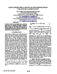
Computational efficiency Fitting CAR and SAR models for large data sets could be computationally challenging, especially for the spatial variance-covariance parameters. Using our new algorithm in hglm, moderately sized problems can be fitted efficiently. We re-sampled from the ohio data set (for more details on the data set see also the examples) for different number of locations, each with 10 replicates, executed on a single Intel© Xeon© E5520 2.27GHz CPU. In each replicate, the data was fitted using both hglm and spaMM, for the same model described above. The results regarding average computational time are summarized in Figure 2. hglm is clearly more usable for fitting larger sized data sets. In the package vignette, we also show the comparisons of the parameter estimates, where the "EQL" estimates from hglm are almost identical

The R Journal Vol. 7/2, December 2015

ISSN 2073-4859

Execution time for CAR model fitting

C ONTRIBUTED R ESEARCH A RTICLES

11

10 min package hglm spaMM

5 min

1 min 30 sec 1 sec 50

100

200

300

400

500

Number of locations

Figure 2: Comparison of the execution time for fitting CAR models using hglm and spaMM. to the "EQL-" estimates from spaMM, with high correlation coefficients between the two methods: 1.0000, 0.9998, 0.9997 and 0.9999 for the residual variance, ρ, τ and the intercept, respectively.

Examples Scottish Lip Cancer data set Here we analyze the cancer data set (source: Clayton and Kaldor, 1987) from the hglm package. Calling data(cancer) loads a numeric vector E that represents the expected number of skin cancer patients in different districts in Scotland, a numeric vector O giving the corresponding observed counts, a numeric vector Paff giving proportion of people involved agriculture, farming, and fisheries, and matrix D giving the neighborhood structure among Scottish districts. Here we demonstrate how the data is fitted as a CAR model or a SAR model, using the hglm package with the EQL method.

> > > > > + + + + >

library(hglm) data(cancer) logE |t|) (Intercept) 0.19579 0.20260 0.966 0.34241 Paff 0.03637 0.01165 3.122 0.00425 ** --Signif. codes: 0 '***' 0.001 '**' 0.01 '*' 0.05 '.' 0.1 ' ' 1 Note: P-values are based on 27 degrees of freedom Summary of the random effects estimates: Estimate Std. Error [1,] 0.7367 1.0469 [2,] 0.6336 0.3930 [3,] 0.4537 0.5784 ... NOTE: to show all the random effects, use print(summary(hglm.object), print.ranef = TRUE). ---------------DISPERSION MODEL ---------------NOTE: h-likelihood estimates through EQL can be biased. Dispersion parameter for the mean model: [1] 1 Model estimates for the dispersion term: Link = log Effects: [1] 1 Dispersion = 1 is used in Gamma model on deviances to calculate the standard error(s). Dispersion parameter for the random effects: [1] 16.3 Dispersion model for the random effects: Link = log

The R Journal Vol. 7/2, December 2015

ISSN 2073-4859

C ONTRIBUTED R ESEARCH A RTICLES

14

Effects: .|Random1

Estimate Std. Error 1/sqrt(SAR.tau) 2.7911 0.4058 -SAR.rho/sqrt(SAR.tau) -0.4397 0.0822 SAR.tau (estimated spatial variance component): 0.1284 SAR.rho (estimated spatial correlation): 0.1575 Dispersion = 1 is used in Gamma model on deviances to calculate the standard error(s). EQL estimation converged in 12 iterations.

For the CAR model, the hglm estimates are exactly the same as those labelled as “PQL” estimates in Lee and Lee (2012). To get the EQL1 correction the user has to add the option method = "EQL1" and the hglm function gives similarresults to those reported in Lee and Lee (2012), e.g., their HL(1,1) estimates 

were intercept, β f pp , τ, ρ = (0.238, 0.0376, 0.155, 0.174) whereas our "EQL1" correction gives (0.234, 0.0377, 0.156, 0.174) (see also Section “Fitting a spatial Markov Random Field model using the CAR family” in the package vignette). A minor difference to the "EQL1" result appears because Lee and Lee (2012) used the HL(1,1) modification to their HL(0,1) whereas we apply such a correction directly to EQL which is slightly different from HL(0,1) (see Table 1).

Ohio elementary school grades data set We analyze a data set consisting of the student grades of 1,967 Ohio Elementary Schools during the year 2001–2002. The data set is freely available on the internet (URL http://www.spatial-econometrics. com/) as a web supplement to LeSage and Pace (2009) but was not analyzed therein. The shape files were downloaded from http://www.census.gov/cgi-bin/geo/shapefiles2013/main and the districts of 1,860 schools in these two files could be connected unambiguously. The data set contains information on, for instance, school building ID, Zip code of the location of the school, proportion of passing on five subjects, number of teachers, number of students, etc. We regress the median of 4th grade proficiency scores, y, on an intercept, based on school districts. The statistical model is given as yi,j = µ + v j + ei,j ,

(16)
2

where i = 1, 2, . . . , 1860 (observations), j = 1, 2, . . . , 616 (districts), ei,j ∼ N 0, σe , {v j } = v ∼   N 0, τ (I − ρW)−1 and W = {w p,q }616 p,q=1 is a spatial weight matrix (i.e., the neighborhood matrix). We construct w p,q = 1 if the two districts p and q are adjacent, and w p,q = 0 otherwise. The above choice of constructing the weight matrix is rather simple. Because the aim of this paper is to demonstrate the use of hglm for fitting spatial models rather than drawing conclusions from real data analysis, we skip any further discussion on the construction of the weight matrix. Interested, readers are referred to LeSage and Pace (2009) for more discussion on the construction of the spatial weight matrices. With the spatial weight matrix defined as above, we can estimate model (16) by using our hglm package in the following way.

> > > > > > > + >

## load the data object 'ohio' data(ohio) ## fit a CAR model for the median scores of the districts X > > + > > > > > +

districtShape