Entropy 2010, 12, 1743-1764; doi:10.3390/e12071743 OPEN ACCESS
entropy ISSN 1099-4300 www.mdpi.com/journal/entropy Article
Fitting Ranked Linguistic Data with Two-Parameter Functions Wentian Li 1,⋆ , Pedro Miramontes 2,4 and Germinal Cocho 3,4 1
Feinstein Institute for Medical Research, North Shore LIJ Health Systems, 350 Community Drive, Manhasset, NY 11030, USA 2 Departamento de Matem´aticas, Facultad de Ciencias, Universidad Nacional Aut´onoma de M´exico, Circuito Exterior, Ciudad Universitaria, M´exico 04510 DF, Mexico; E-Mail:
[email protected] 3 Departamento de Sistemas Complejos, Instituto de F´ısica, Universidad Nacional Aut´onoma de M´exico, Apartado Postal 20-364, M´exico 01000 DF, Mexico; E-Mail:
[email protected] 4 Centro de Ciencias de la Complejidad, Universidad Nacional Aut´onoma de M´exico, Circuito Escolar, Ciudad Universitaria, M´exico 04510 DF, Mexico ⋆
Author to whom correspondence should be addressed; E-Mail:
[email protected]; Tel.: +1 516 562 1076; Fax: +1 516 562 1153.
Received: 4 April 2010; in revised form: 18 May 2010 / Accepted: 1 July 2010 / Published: 7 July 2010
Abstract: It is well known that many ranked linguistic data can fit well with one-parameter models such as Zipf’s law for ranked word frequencies. However, in cases where discrepancies from the one-parameter model occur (these will come at the two extremes of the rank), it is natural to use one more parameter in the fitting model. In this paper, we compare several two-parameter models, including Beta function, Yule function, Weibull function—all can be framed as a multiple regression in the logarithmic scale—in their fitting performance of several ranked linguistic data, such as letter frequencies, word-spacings, and word frequencies. We observed that Beta function fits the ranked letter frequency the best, Yule function fits the ranked word-spacing distribution the best, and Altmann, Beta, Yule functions all slightly outperform the Zipf’s power-law function in word rankedfrequency distribution. Keywords: Zipf’s law; regression; model selection; Beta function; letter frequency distribution; word-spacing distribution; word frequency distribution; weighting
Entropy 2010, 12
1744
1. Introduction Empirical linguistic laws tend to be functions with one key parameter: Zipf’s law [1], which describes the relationship between the number of occurrence of a word (f ) and the resulting ranking of the word from common to rare (r), states that f ∼ 1/ra , with the scaling exponent a as the free parameter. Herdan’s or Heaps’ law describes how the number of distinct words used in a text (V , or “vocabulary size”, or number of types) increases with the total number of appearance of words (N , or, the number of tokens) as: V ∼ N θ [2,3]. Although in both Zipf’s and Herdan’s law, there is a second parameter: f = C/ra , V = CN θ , the parameter C is either a y-intercept in linear regression and thus not considered to be functionally important, or subtracted from the total number of parameters by the normalization ∑ constraint (e.g., i (fi /N ) = 1). Interestingly, one empirical linguistic law, the Menzerath-Altmann law [4,5], concerning the relationship between the length of two linguistic units, contains two free parameters. Suppose the higher linguistic unit is the sentence, whose length (y) is measured by the number of the lower linguistic unit, words, and the length of words (x) is measured by the even lower linguistic unit, e.g., phonemes or letters. Then, the Menzerath-Altmann law states that y ∼ xb e−c/x with two free parameters, b and c. Few people paid attention to the two-parameter nature of this function as it does not fit the data as good as the Zipf’s law on its respective data, although Baayen listed several multiple-parameter theoretical models in his review on word frequency distribution [6]. We argue here about need to apply two-parameter functions to fit ranked linguistic data for two reasons. First, some ranked linguistic data, such as the letter usage frequencies, do not follow well a power-law trend. It is then natural to be flexible in data fitting by using two-parameter functions. Second, even for the known cases of “good fits”, such as the Zipf’s law on ranked word-frequency distribution i.e., rank-frequency plot), the fitting tends to be not so good when the full ranking range is included. This imperfection is more often ignored than investigated. We would like to check whether one can model the data even better than Zipf’s law by using two-parameter fitting functions. The first 2-parameter function we consider is the Beta-function which attempts to fit the two ends of a rank-frequency distribution by power-laws with different exponents [7,8]. Suppose the variable f values are ranked: f(1) ≥ f(2) ≥ f(3) · · · ≥ f(n) , we define the normalized frequencies p(r) ≡ f(r) /N ∑ such that nr=1 f(r) = 1, (n denotes the number of items to be ranked, r denotes the rank number, and ∑ N = nr=1 f(r) is the normalization factor). In a Beta function, the ranked distribution is modeled by Beta:
p(r) = C
(n + 1 − r)b ra
(1)
where the parameter a characterizes the scaling for low-rank-number (i.e., high frequency) items points, and b characterizes the scaling for the high-rank-number (i.e., low frequency) items points. For the example of English words, n is the vocabulary size, and “the” is usually the r = 1 (most frequent) word. If a logarithmic transformation is applied to both sides of Equation (1), the Beta function can be cast in a multiple regression model: Beta (linear regression form):
log(p(r) ) = c0 + c1 log(r) + c2 log(r′ )
where r′ = n + 1 − r, c1 = −a, c2 = b, and c0 = log(C).
(2)
Entropy 2010, 12
1745
The second 2-parameter function we are interested in is the Yule-function [9]: p(r) = C
Yule:
br ra
(3)
A previous application of Yule’s function to linguistic data can be found in [10]. The Menzerath-Altmann function mentioned earlier: p(r) = Crb e−a/r
Menzerath-Altmann:
(4)
cannot be guaranteed to be a model for ranked distribution as the monotonically decreasing property is not always true even when the parameter b stays negative. Note that Menzerath-Altmann function is a special case of f = Crb exp(−a/r − d · r) which shares the same functional form as the generalized inverse Gauss-Poisson distribution [6]. Another two-parameter function, proposed by Mandelbrot [11], cannot be easily cast in a regression framework, and it is not used in this paper: Mandelbrot:
p(r) =
A (r + b)a
(5)
For random texts, one can calculate the value of b, e.g., b = 26/25 = 1.04 for 26-alphabet languages [12]. Clearly, all these 2-parameter functions one way or the other attempt to modify the power-law function: C power-law, Zipf: p(r) = a (6) r For comparison purposes, the exponential function is also applied: exponential:
p(r) = Ce−ar
(7)
Two more fitting functions, whose origin will be explained in the next section, are labeled as Gusein-Zade [13] and Weibull functions [14]: ( ) n+1 Gusein-Zade: p(r) = C log (8) r (
))a n+1 Weibull: p(r) = C log (9) r In this paper, these functions will be applied to ranked letter frequency distributions, ranked word-spacing distributions, and ranked word frequency distributions. A complete list of functions, their corresponding multiple linear regression form, and the dataset each function will be applied, are included in Table 1. When the normalization factor N is fixed, parameter C is no longer freely adjustable, and the number of free parameters, K − 1, is one less the number of fitting parameters, K. The value of K − 1 is also listed in Table 1. The general framework we adopt in comparing different fitting functions is Akaike information criterion (AIC) [15] in regression models. In regression, model parameters in model y = F (x) are estimated to minimize the sum of squared errors (SSE): SSE =
(
n ∑ (yi − F (xi ))2 i=1
(10)
Entropy 2010, 12
1746
It can be shown that when the variance of the error is unknown, which is to be estimated from the data, ˆ (the underlying statistical model is that the fitting noise or least square leads to maximum likelihood L deviance is normally distributed) (p. 185 of [16]): ˆ = C − n log SSE − n L 2 n 2 The model selection based on AIC minimizes the following term:
(11)
ˆ + 2K AIC = −2L
(12)
where K is the number of fitting parameters in the model. Combining the above two equations, it is clear that AIC of a regression model can be expressed by SSE (any constant term will be canceled when two models are compared, so it is removed from the definition): SSE + 2K n For two models applied to the same dataset, the difference between their AIC’s is: AIC = n log
AIC2 − AIC1 = n log
(13)
SSE2 + 2(K2 − K1 ) SSE1
(14)
If model-2 has one more parameter than model-1, model-2 will be selected if SSE2 /SSE1 < e−2/n . Note that almost all fitting functions listed in Table 1 are variations of the power-law function, so the regression model is better applied to the log-frequency scale: y = log(p). Table 1. List of functions discussed in this paper. The number of free parameters in a function is K − 1. The functional form in the third and the 4th column is for p(r) = f(r) /N , or log(p(r) ), respectively. We define: x1 = log(r), x2 = log(n + 1 − r), x3 = 1/r, and x4 = log(log((n + 1)/r)). The last 3 columns indicate which dataset a function is applied to (marked by x): dataset 1 is the ranked letter frequency distribution, dataset 2 is the ranked inter-word spacing distribution, and dataset 3 is the ranked word frequency distribution. model
K −1
formula (p(r) = f(r) /N )
linear regression (y = log p(r) )
data1 (letter freq.)
data2 (word spacing)
data3 (word freq.)
Gusein-Zade Weibull power-law exponential Beta Yule Altmann Mandelbrot
0 1 1 1 2 2 2 2
C log((n + 1)/r) C(log((n + 1)/r))a C/ra Ce−ar C(n + 1 − r)b /ra Cbr /ra Crb e−a/r C/(r + b)a
c0 + x4 c0 + c4 x4 c0 + c1 x1 c0 + cr r c0 + c1 x1 + c2 x2 c0 + cr r + c1 x1 c0 + c1 x1 + c3 x3 -
x x x x x x x -
x x x x x x -
x x x x -
Before we fit and compare various functions, we would like to explain the origin of Gusein-Zade and Weibull function by showing the equivalence between an empirical ranked distribution and the empirical cumulative distribution in the next section.
Entropy 2010, 12
1747
2. Equivalence between an Empirical Rank-Value Distribution (eRD) and an Empirical Cumulative Distribution (eCD) Our usage of rank-frequency distribution may raise a question of “why not use a more standard statistical distribution?” It is tempting to relate a sample-based (empirical) ranked distribution to the “order statistics” [17]. However, they are not equivalent. Suppose a particular realization of the values of n variables being ranked (ordered) such that: x(1) > x(2) > x(3) · · · > x(n) , and there are many (e.g., m) realizations; the distribution of m top-ranking (rank-1, order-1, maximum) variable values ({xi(1) }, i = 1, 2, · · · m) characterize an order statistic an empirical rank-value distribution (x-axis: (1, 2, · · · n), y-axis: (x(1) , x(2) , · · · x(n) )) only characterizes the distribution of one particular realization. However, empirical rank-value distribution (eRD) is equivalent to the empirical cumulative distribution (eCD) of the n values of variable x from a data set. Figure 1 shows a step-to-step transformation (starting from the upper-right, counter-clockwise) from an eRD to an eCD, using n = 100 values randomly sampled from the log-normal distribution. One empirical rank-value distribution in Figure 1(A) is transformed to Figure 1(B) by a mirror image with respect to the y-axis, plus a transformation of the x-axis: the new x-axis is reversed from the old x-axis and is normalized to (0,1). The purpose of this operation is to start the empirical cumulation from the lowest ranking point. Figure 1(C) is a mirror image of Figure 1(B) with respect to x-axis, and Figure 1(D) is a counter-clockwise rotation of Figure 1(C) of 90◦ . Figure 1(D) is then the empirical cumulative distribution of this data set, which shows the proportion of values that are smaller than a threshold marked by the x-axis. Actually, there is a simpler operation from Figure 1(A) to Figure 1(D): a clockwise rotation of 90◦ plus a reverse and a normalization of the old x-axis to the new y-axis in the range of (0,1). The relationship between eRD and eCD has been discussed in the literature a number of times [18–23]. The reason we emphasize this relationship is to reinforce the understanding that a functional fitting of the rank-value distribution will correspond to a mathematical description of the empirical cumulative distribution, and vice versa. Since the derivative of the empirical cumulative distribution is the empirical probability density (ePD), we then have an estimation of ePD as well, even though it may not be in a close form. The relationship between an ePD and the true underlying distribution is always tricky [6,24]. The frequency spectrum (FS) [6] is defined as the number of different events occurring with a given frequency. The cumulative sum of FS, called empirical structural type distribution (eSTD), is closely related to the empirical cumulative distribution. Generally speaking, eCD can be converted to eSTD by mirroring with respect to the y = 1 line, then rescale the new y-axis from 1 to n (see Figure 1(D)). The situation is slightly more complicated when there are horizontal bars in eRD (equivalent to vertical lines in eCD) (see section 5). In that case, a horizontal bar is coverted to a point by its right end, before the mirror/rotation is carried out. We note that Alfred James Lotka used FS in his discovery of the power-law pattern in data [22,25].
Entropy 2010, 12
1748
Figure 1. (A) n = 100 log-normal distributed values being ranked (x-axis is the rank r, r = 1 for the largest value, r = n for the smallest value, y-axis is the value itself); (B) Mirror image of (A) with respect to the y-axis. Note that the new x-axis is both reversed and normalized (so that lowest ranking value at 0 and highest ranking value at 1); (C) Mirror image of (B) with respect of x-axis; (D) Rotation of (C) of −90◦ . The highest ranking value is marked by the red color and the lowest ranking value by the blue color. empirical rank−value dist.(eRD)
(A)
4 0
2
x=value
6
8
(B)
0.0
0.2
0.4
0.6
0.8
1.0
0
20
40
(n+1−r)/(n+1)
0.2
0.4
0.6
80
100
r=rank
0.8
empirical cumulative dist.(eCD)
1.0
0.8 0.6 0.4 0.2
cumulative prob
1.0
0.0
60
(C) 0.0
(D)
0
2
4
6
8
10
value
The Gusein-Zade and Weibull function introduced in section 1 can be understood by a reverse transformation from eCD to eRD. Suppose an eCD converges to 1 exponentially, which also describes the gap length distribution of a Poisson process with the mean gap length of fm : f
CD = 1 − e− fm
(15)
Similar to the survival curve in biostatistics [26], eCD is a step function with n vertical jumps. The lowest-ranking point (r = n) corresponds to the first step, with cumulative probability of 1/(n + 1), and the highest-ranking point (r = 1) corresponds to the last step with the cumulative probability of n/(n + 1). This can be used to rewrite Equation (15) as: f(r) n+1−r = 1 − e− fm n+1
(
or, f(r) = fm log
n+1 r
(16)
) (17)
Entropy 2010, 12
1749
which is exactly Equation(8). In data fitting, we treat any coefficient in the function as a parameter, thus fm /N becomes C. This rank-frequency distribution is exactly the same as the one proposed by Sabir Gusein-Zade [13,27,28]. Suppose the CD approaches 1 in a stretched exponential relaxation [29,30]: f
CD = 1 − e−( fm )
α
(18)
the converted RD is the Weibull function defined in Equation(9) with C = fm /N and a = 1/α. In general, any cumulative distribution of f n+1−r = CD(f ) n+1 can be converted to RD by solving f as a function of r.
(19)
3. Ranked Letter Distribution The frequency of letters in a language is of fundamental importance to communication and encryption. For example, the Morse code is designed so that the most common letters have the shortest codes. Shannon used the frequencies of letters as well as other units to study the redundancy and predictability of languages [31]. It is well known that the letter “e” is the most frequent letter in English [32,33]. On the other hand, the most common letter in other languages can be different, e.g., “a” for Turkish, and “a”, “e”, “i” share the top ranks in Italian, etc. ( http://en.wikipedia.org/wiki/Letter frequency) We plot the ranked letter frequencies in the text of Moby Dick in Figure 2 both in linear-linear and log-log scales (see Appendix A for the source information). The number of bits in Morse code for these letters is also listed in Figure 2(A), which does show the tendency of low number of bits for more commonly used letters. Seven fitting functions (one zero-parameter, three one-parameter, and three two-parameter functions) are applied (Table 1). All can be framed in multiple regression (see Appendix B for programming information). The fitting of Gusein-Zade equation in a regression for the log-frequency data needs more explanation. From Table 1, we see that there is no regression coefficient for the x4 = log log(27/r) term, and the only parameter to be estimated is the constant term. To show this fact, the regression model is re-written as: p(r) = c0 (20) log(p(r) ) − x4 = log log((n + 1)/r) From Figure 2, it is clear that power-law, Altmann, and Yule functions do not fit the data as well as other functions. When the one-parameter functions are compared, exponential function clearly out-performs the power-law function. For regression on the log-frequency data, SSE and AIC can be determined, and conclusion on which model is the best model can be reached. Table 2 shows that Beta function is the best fitting function, followed by Weibull and Gusein-Zade function. The performance of Gusein-Zade function is impressive, considering that it has 2 fewer parameters than Beta and Weibull functions. Another commonly used measure of fitting performance is R2 , which does ignore the issue of number of parameters. R2 can either be defined as the proportion of variance “explained” by the regression or defined as the squared correlation between the observed and the fitted values (see Appendix C for more details).
Entropy 2010, 12
1750
Figure 2. Ranked letter frequency distribution for the text of Moby Dick (normalized so that ∑ the sum of all letter frequencies is equal to 1: p(r) = f(r) / i f(r) ). (A) in the linear-linear scale, and (B) in log-log scale. Seven fitting functions (see Table 1) are overlapped on the data: power-law function (brown, a = 1.34), exponential (lightblue, a = 0.175), Beta function (red, a = 0.0886, b = 1.64), Yule function (blue, a = −0.938, b = 0.764), Gusein-Zade (green), Weibull (purple, a = 1.27), and Altmann (pink, a = 5.78, b = −2.58). The number of bits in Morse code for the corresponding letter is written at the bottom of (A). 2 2 The R2 values listed are Rcor or Rcor,log in Equation (26).
0.15 0.10
e a
o n
i
h s
r
l
d
Yule: R2cor=0.79 Altmann: R2cor=0.63 PowerLaw: R2cor=0.58
u m c w g f p y b
num. bits in the Morse code 1
0
1
2
3
2
2
4
5
e
5e−02
5e−01
0.00
0.05
t
(A) linear−linear
Beta: R2cor=0.97 Gusein−Zade: R2cor=0.96 Weibull: R2cor=0.93 Exponential: R2cor=0.92
3
3
4
5e−03
3
2
4
3
3
4
4
4
15
4
v k q
j
x z
3
4
4
4
4
20
4
25
(B) log−log t
a
Beta: R2cor.log=0.95 Weibull: R2cor.log=0.93 Gusein−Zade: R2cor.log=0.93
1
3
10
5e−04
normalized letter frequency [log]
normalized letter frequency
ranked letter frequency distribution −− Moby Dick
2
o
n
i
h s r l d u m c wg f py
Yule: R2cor.log=0.87 Exponential: R2cor.log=0.83 Altmann: R2cor.log=0.72 PowerLaw: R2cor.log=0.59
5
10
b vk q
jx z
20
rank [log]
The R2 values in Table 2 show again that Beta function is the best fitting function, followed by 2 2 Weibull and Gusein-Zade functions. The Rlog and Rcor,log for Gusein-Zade function is not equal because the variance decomposition does not hold true (Appendix C) when Equation (20) is converted back to the form of log(p(r) ) = c0 + x4 . When the regression is carried out in log-frequency scale, whereas the SSE and R2 is calculated in the scale, we do not expect the variance decomposition holds true, and do not expect R2 to be equal to 2 2 for these models when y axis in linear scale. . The last two columns in Table 2 shows SSE and Rcor Rcor There are a few minor changes in the relative fitting performance among different functions. However, we caution in reading too much in these numbers as the parameter values are fitted to ensure the best performance in the log-frequency scale, not in the frequency scale.
Entropy 2010, 12
1751
Table 2. Comparison of regression models in fitting ranked letter frequency distribution obtained from the text of Mody Dick. The regression is applied to the log-frequency scale (Table 1). SSE: sum of squared error (Equation (10)); ∆AIC: Akaike information criterion 2 relative to the best model (whose AIC is set at 0) (Equation (14)); Rlog : variance ratio 2 2 Equation (25); Rcorr,log : an alternative definition of R based on correlation (Equation (26)). 2 The SSE and Rcor , based on the regression in the logarithmic scale, whereas applied to the linear y scale, are shown in the last two columns. model Gusein-Zade power-law exponential Weibull Beta Yule Altmann
K −1 0 1 1 1 2 2 2
log-scale 2 SSE ∆ AIC Rcor,log 5.77 16.9 0.933 22.2 53.9 0.586 8.91 30.2 0.834 3.59 6.52 0.933 2.58 0 0.952 6.66 24.6 0.876 14.83 47.4 0.723
2 Rlog
0.892 0.586 0.834 0.933 0.952 0.876 0.723
linear-scale 2 SSE Rcor .00196 0.962 0.145 0.580 0.0124 0.918 .00726 0.928 .000716 0.973 .00752 0.795 0.0323 0.628
The fitted Beta function in Figure 2(B) is: log(p(r) ) = −7.5254 + 1.6355 log(27 − r) − 0.08856 log(r)
(21)
i.e., the two parameters in Equation (1) are a ≈ 0.09 and b ≈ 1.6. In [34], the relative magnitude of a and b is used to measure the consistency to power-law behavior (a >> b provides a confirming answer, and a