FixMe: A Self-organizing Isolated Anomaly Detection Architecture for Large Scale Distributed Systems Emmanuelle Anceaume, Romaric Ludinard, Bruno Sericola, Erwan Le Merrer, Gilles Straub
To cite this version: Emmanuelle Anceaume, Romaric Ludinard, Bruno Sericola, Erwan Le Merrer, Gilles Straub. FixMe: A Self-organizing Isolated Anomaly Detection Architecture for Large Scale Distributed Systems. Proceedings of the 16th International Conference On Principles Of Distributed Systems (OPODIS), Dec 2012, Rome, Italy. pp.12, 2012.
HAL Id: hal-00736922 https://hal.archives-ouvertes.fr/hal-00736922 Submitted on 30 Sep 2012
HAL is a multi-disciplinary open access archive for the deposit and dissemination of scientific research documents, whether they are published or not. The documents may come from teaching and research institutions in France or abroad, or from public or private research centers.
L’archive ouverte pluridisciplinaire HAL, est destin´ee au d´epˆot et `a la diffusion de documents scientifiques de niveau recherche, publi´es ou non, ´emanant des ´etablissements d’enseignement et de recherche fran¸cais ou ´etrangers, des laboratoires publics ou priv´es.
FixMe: A Self-organizing Isolated Anomaly Detection Architecture for Large Scale Distributed Systems Emmanuelle Anceaume1 , Erwan Le Merrer2 , Romaric Ludinard3 , Bruno Sericola3 , and Gilles Straub2 1
IRISA / CNRS (France),
[email protected] Technicolor Rennes (France),
[email protected] Inria Rennes - Bretagne Atlantique (France),
[email protected] 2
3
Abstract. Monitoring a system is the ability of collecting and analyzing relevant information provided by the monitored devices so as to be continuously aware of the system state. However, the ever growing complexity and scale of systems makes both real time monitoring and fault detection a quite tedious task. Thus the usually adopted option is to focus solely on a subset of information states, so as to provide coarse-grained indicators. As a consequence, detecting isolated failures or anomalies is a quite challenging issue. In this work, we propose to address this issue by pushing the monitoring task at the edge of the network. We present a peer-to-peer based architecture, which enables nodes to adaptively and efficiently self-organize according to their “health” indicators. By exploiting both temporal and spatial correlations that exist between a device and its vicinity, our approach guarantees that only isolated anomalies (an anomaly is isolated if it impacts solely a monitored device) are reported on the fly to the network operator. We show that the end-to-end detection process, i.e., from the local detection to the management operator reporting, requires a logarithmic number of messages in the size of the network.
1
Introduction
The number of IP-enabled devices keeps on growing in a steady manner, often reaching millions of units managed by a single operator. If those devices are able to provide a service to the user in their intended running state, deviations in behavior or hardware/software problems are generally detected offline by human intervention. The technical barrier for efficient online monitoring and analysis is the size of the devices set to operate, together with the huge amount of parameters and states to consider. Network operators deploy helpdesk in order to support their customers when they are facing problems. In the last years the cable and telecom industry have developed different remote management standards [1] to better support the helpdesk operator via dedicated protocols and tools. As a consequence, the helpdesk operation represents an important part of the overall operating cost of a network provider. Reducing
the number of calls as well as their duration is an important key for every network operator to sustain profitability and reduce the total cost of ownership. Nevertheless both telecom and cable industries came up with client-server architectures where a single server (or a farm of servers) is in charge of managing a set of devices. Such architectures are typically used for management tasks (e.g., service provisioning, device firmware upgrading) rather than for real time monitoring activities, essentially because of scaling issues. Indeed, the massive scale we are considering calls for efficient monitoring algorithms. A first option is to gather all the devices logs in a single place, and to analyze collected data using for instance the MapReduce paradigm [2] to detect the causes of the anomalies. This nevertheless implies a significant detection latency and processing cost at the cloud architecture level. The second option is to push monitoring procedures on devices. Actually, standardized procedures exist at devices level to autonomously trigger asynchronous alarms in presence of anomalies. However, these procedures are never used for practical reasons. Indeed if the cause of the anomaly lies in the network itself (e.g., at routers, links or data center outages) this may impact a very large number of devices, and thus letting thousands of impacted devices reporting the problem to the helpdesk operator may quickly become a disaster due to the volume of generated messages. On the other hand, it is of utmost importance to minimize the overall network footprint by giving each device the capability to self distinguish network-based anomalies from isolated ones – anomalies that only impact the device itself – so that only isolated anomalies are reported on the fly to the helpdesk. This is the problem that we address in this paper. Specifically, we propose a novel distributed monitoring tool, called FixMe, that enjoys the following properties. – FixMe is self-managing: all the monitored devices self-organize according to their “health” indicators so that they can detect any correlation between their state and the one of their neighbors, – FixMe is dynamic: (i) monitored devices may join the system or may be removed from it at any time, and (ii) there is no assumption regarding the QoS repartition of the monitored nodes (i.e., we do not assume that the repartition is uniform), – FixMe does not rely on any complex bootstrap procedure. In contrast to most of the monitoring tools, devices do not need to be prearranged into a predefined number of clusters (as required for in instance in k-means based solutions), – FixMe is scalable: the end-to-end detection process, i.e. from the local detection to the management operator reporting, requires a logarithmic number of messages. The remaining of the paper is organized as follows. Section 2 provides an overview of existing monitoring approaches. Section 3 presents the model of the system, and defines the addressed problem. Section 4 describes the FixMe overlay and its associated operations, while in Section 5 its efficiency is analyzed. Section 6 describes the algorithm that solves the addressed problem. Section 7 concludes and presents future works.
2
Related work
This Section provides an overview of the existing techniques used in large scale systems to continuously and automatically monitor time-varying metrics. The authors in [3] exploit temporal and spatial correlations [4– 6] among groups of monitored nodes to decrease monitoring communication costs, i.e., the cost incurred by the periodic reporting of the updated metrics values from the monitored nodes to the management node. The idea is to prevent any reporting message from occurring when such a reporting would contain metrics values that could be directly inferred by the management node. This is achieved by giving each monitored node the capability to locally detect whether the current values of its monitored metrics are in accordance with predicted ones (through Kalman filters tools [7] installed at both monitored nodes and the management node), and by gathering nodes into clusters (such that, for each monitored metric, a set of clusters group together nodes that share correlated values of the considered metric according to the Pearson correlation coefficient). At clusters level, an elected leader is in charge of communicating with the management system when the current metric values of its group members differ from each others. Although close to our objectives, the main drawback of this solution lies on the centralized clustering process. All the nodes of the system are continuously organized into clusters computed through the k-means algorithm exclusively run by the management node, which is a clear impediment to the scalability of their approach. Other works aim at minimizing the processing cost for continuous monitoring [8–10] in the light of the theoretical results of [11], however similarly to [3], all these approaches suffer from a centralized handling of the clustering process. In contrast, our objective is a fine-grain detection tool capable of accurately and efficiently detecting isolated events. As will be described in the remaining of the paper, we combine clustering and structured peerto-peer architectures to tend toward this objective.
3
Model of the System
We consider a set of N nodes that communicate among each other through the standard synchronous message-passing model. Each node in the system is assigned a unique random identifier derived from a standard hash function (e.g. MD5, SHA-1). Each node has access to D services numbered 1, . . . , D. At any time t, the QoS of each service is locally measured with an end-to-end performance measurement function Qi : {1, . . . , N } × N −→ [ai , bi ] (p, t) 7−→ Quality of service i at node p at time t Without loss of generality we suppose that the QoS range [ai , bi ] of service i is equal to [0, 1]. We define the position of a node p at time t by the vector Q(p, t) defined as Q(p, t) = (Q1 (p, t), . . . , QD (p, t)).
(1)
For each monitored service i = 1, . . . , D, we split interval [0, 1] into ni (j−1) (j) (0) (n ) disjoint intervals [xi , xi ), 1 ≤ j ≤ ni , with xi = 0 and xi i = 1, the last interval being closed. Integer ni is a parameter of the system. These ni intervals can be thought as ni QoS classes of service i. For (j) instance, one can consider a division of [0, 1] for service i such that |xi − (j−1) (j+1) (j) xi | ≥ |xi − xi |. Such a division could be used to reflect the increasing sensitivity of users regarding QoS variations. A user is more sensitive to a very small variation of a high QoS than to a large variation of a low QoS. Without loss of generality, we suppose a regular division (j) (j−1) into identical length intervals and we define ρi = |xi −xi | = 1/ni . In the following these intervals are named buckets (a more precise definition is given in Section 4). In addition to the functions Q1 , . . . , QD , each node has access to D anomaly detection functions A1 , . . . , AD . At each time t, each function Ai is fed with the sequence of the ℓi ≥ 1 last QoS values Qi (p, t − ℓi + 1), . . . , Qi (p, t) and provides some meaningful prediction of what should be the next QoS value. Note that ℓi is a parameter of Ai . These functions are implemented to cope with the specific variations of their input values, and thus different kinds of anomaly detection functions exist, ranging from a simple threshold based functions, to more sophisticated ones like the Holt-Winters forecasting or Cusum method. In this paper, we suppose that the output of these anomaly detections are boolean. At time t, Ai (p, t) = true if the sequence Qi (p, t − ℓi + 1), . . . , Qi (p, t) is considered as an anomaly, it is false otherwise. Implementation of both Qi and Ai functions are out of the scope of the paper. Finally, suppose that a node locally detects an anomaly whose origin comes from a network/service dysfunction or failure. Then this anomaly will have an impact on the QoS of other nodes, and thus these nodes will locally detect it. On the other hand, we suppose that if a node locally detects an anomaly whose origin is local (hardware or software), then this anomaly will only impact its QoS, and thus no other nodes will be impacted by this specific anomaly. Prior to defining the addressed problem, let us consider the following simple scenario presented in Fig. 1. The QoS of a single service monitored by two nodes a and b is represented by interval [0, 1]. At time t the quality positions Q(a, t) and Q(b, t) of both nodes lie in bucket j, while at time t + 1, at least one of the two nodes experience a QoS change. Five situations can be observed. In situations (1), (2) and (4) node a is the only node that observes a QoS change. In situation (1), this change does not push a position outside bucket j, while in situation (2) and (4) it does. However in both situations (1) and (2), the anomaly detection function A1 (a, t + 1) = false, thus a does not consider this move as an anomaly, therefore does not do any more investigation. In the other hand, in situation (4), A1 (a, t + 1) = true, and thus node a triggers a FixMe message. Now observe the two last situations (3) and (5). Both nodes observe a QoS change considered as an anomaly by their function A (i.e., A1 (a, t + 1) = A1 (b, t + 1) = true). However in situation (3) the QoS degradation is the same for both nodes (Q(a, t+1) and Q(b, t+1) lie in bucket k) and thus neither a nor b consider this anomaly as isolated, while in situation (5) Q(a, t+1) and Q(b, t+1) respectively lie in buckets
a b
t
j (1)
t+1
(2) a
a b j
(3) b
a
kj k No FixMe Alerts
(4) b j
a k
(5) b
a
b
j kℓ FixMe Alerts
j
Fig. 1. Isolated anomaly detection of one monitored service. Node a triggers FixMe message in both cases (4) and (5), while node b triggers it only in case (5).
k and ℓ. Thus both nodes trigger a FixMe message. We now formally define the problem we address in this work. Definition 1 (The Isolated Anomaly Detection Problem). Let S = {1, . . . , N } be the set of monitoring nodes, and an additional node named the management operator with which any of the N nodes commut t ⊆ S be such that ∀p ∈ Sj,k , p has moved from bucket j to nicate. Let Sj,k bucket k from time t − 1 to time t and there exists a service i such that Ai (p, t) = true. Then at time t + 1, an alert is raised at the management t operator if and only if |Sj,k | ≤ τ , with τ a parameter of the system. In Fig. 1, τ = 1.
4 4.1
FixMe Framework Rationale
In this Section, we describe how we address the Isolated Anomaly Detection problem in a distributed system composed of N monitored nodes. FixMe framework orchestrates the monitored nodes into an overlay network, named in the following FixMe overlay. An overlay network is actually a virtual network built on top of the physical network within which nodes communicate among each other along the edges of the overlay by using the communication primitives provided by the underlying network (e.g. IP network service). The algorithms nodes use to choose their neighbors and to route their messages define the overlay topology. The topology of unstructured overlays conforms with random graphs (i.e., relationship among nodes are mostly set according to a random process which reveals to be inefficient to find a particular node or set of nodes in the overlay). On the other hand, structured overlays build their topology according to structured graphs (e.g., tree, torus, hypercube). Most of the structured overlays are based on Distributed Hash Tables (e.g., [12, 13]).
The efficiency and scalability of all these proposed DHTs rely on the uniform distribution of the nodes in the identifiers space at the expense of breaking the application logic. This is why, for specific applications such as streaming applications, broadcast spanning trees structures, that support the application-level broadcast, have been proposed [14]. Our concern is to exploit the QoS relationship among monitored nodes, which make all the aforementioned solutions non adapted. As a consequence, we propose to organize nodes so that at any time t the neighbors of any node p are the nodes q whose QoS (i.e. Q(q, t)) are closer to the QoS of p (i.e. Q(p, t)). The description of such an organization is done in Section 4.2. From the application point of view, three operations are provided by the system: the lookup, the join, and leave operations that allow nodes to respectively find a position in the overlay, join the overlay or leave it. From the topological structure point of view, two operations are provided: the split and merge operations that guarantee the scalability of FixMe overlay when some regions of the overlay become too dense or too sparse. All these operations are described in Section 4.3. Finally, when too many monitored nodes share exactly the same QoS (or equivalently sit at the same position in the overlay), nodes within the bucket self-organize into an hypercube as described in Section 4.4.
4.2
Overview of FixMe Overlay
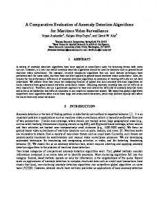
The FixMe overlay is a virtual multi-dimensional cartesian coordinate space on a multi-torus. The entire coordinate space is tessellated into a collection of buckets. A bucket is the cartesian product of D intervals of respective length ρ1 , . . . , ρD (cf. Fig. 2, where FixMe overlay is made of 162 buckets). When a node p joins FixMe at time t, p joins the bucket which corresponds to its quality position (or simply its position) Q(p, t). When a bucket is populated by more than Smin nodes this bucket is called a seed. The entire coordinate space is dynamically partitioned into distinct zones, named cells, such that a cell contains at most one seed (cf. Fig. 2, where FixMe overlay on the left is made of four cells, and the one on the right is made of five cells). More formally, Definition 2 (Cell). A cell is defined as an hyper-rectangle of buckets, among which at most one is a seed. A cell is fully and uniquely characterized by a set of 2D buckets called the corners of the cell, sorted using the lexicographic order. Figure 2 shows these different elements for D = 2 and ρ1 = ρ2 = 1/16. The buckets are elementary squares, the seeds are represented by the black squares, and the cells are depicted by the coloured rectangles. Note that neither cell 4 (on the figure on the left) nor cell 5 (on the figure on the right) have a seed. The reasons will be detailed in the following.
4.3
FixMe Operations
Lookup operation. We describe how a node locates the seed that is in charge of a given bucket b through the lookup operation. In FixMe,
y
y
1
1 Cell3
Cell4
Cell4
Cell5
′
Cell3 s hook 1 2
1 2
Cell3 Seed Cell1 O
Cell2 1 2
1
x
Cell1 O
Cell2 1 2
1
x
Fig. 2. FixMe overlay before (on the left) and after (on the right) a split operation
routing is exclusively handled by seeds. Each seed maintains a routing table that contains an entry for each of its 2D neighboring seeds in the coordinate space. An entry contains the IP address and the virtual coordinate of the seed. A lookup message contains the destination coordinates. Using the neighbor coordinate, a seed routes a lookup message toward its destination using a simple greedy forwarding to the neighbor seed that is closest to the destination address. CAN [12] uses this routing to cross its zones. However, as such the lookup operation needs to cross in average O(DN 1/D ) zones. We combine the multidimensional routing of CAN with Chord-fashioned long-range neighbors [13, 15] to improve the lookup operation cost. Specifically, in addition to its 2D neighboring seeds, each seed associates a location key to each neighbor seed of its routing table. Hence, if the seed coordinates are (x1 , . . . , xd , . . . , xD ), then the +ith (respectively the −ith) key location for the dth axis is defined by (x1 , . . . , x(d,+i) , . . . , xD ), where x(d,+i) = xd + 2i ρd (respectively x(d,−i) = xd − 2i ρd ). In addition, the distance between the seed and the location key is bounded by Rd where Rd is a system parameter corresponding to the absolute farthest location to be accessed in one hop in the dth axis. Each seed s also maintains a predecessors table that contains couples (s′ , l), where s′ is a seed pointing on location l in s cell. The predecessors table is used when a split or merge operation are triggered to update the predecessors routing table.
Join operation. When some new node p wants to join the system at time t, it contacts some node q already in the system. This bootstrap node q sends a lookup request for the incoming node position Q(p, t) to find the seed s responsible for the cell in which p must be inserted. Once p gets s address, it asks s to join the bucket that matches its position Q(p, t). If that bucket is the seed s itself, then the procedure described in Section 4.4 is run. Otherwise, s updates its cell routing table by inserting p address and its position Q(p, t). Similarly, p keeps a pointer to s (as described above, routing is handled by seeds, thus p only needs to point to s). Now, if the number of nodes that sit in p bucket exceeds Smin
Algorithm 1: p.join(t,q=None) 1 2 3 4 5 6 7 8 9 10 11 12 13 14 15
begin if q = None then q ← getBootstrapNode() ; end seed ← q.lookup(Q(p,t)); if p ∈ seed then seed.insert(p); else bucket ← seed.findBucket(p); bucket.insert(p); if | bucket |≥ Smin then cells ← seed.split(bucket); end end end
Algorithm 2: cell.merge(bucket) 1 2 3 4 5 6
Data: bucket such that| bucket |< Smin begin seed ← cell.seed; seed.addOrphanCell(bucket.cell); seed.mergeSiblingsCells(); seed.notifyPredecessors(bucket.cell); end
Algorithm 3: cell.split(bucket)
1 2 3 4 5 6 7 8 9
Requires: | bucket |≥ Smin ∧ ¬bucket.isSeed() Ensures : bucket.isSeed() begin matchingCell ← findCell(bucket); if matchingCell ∈ orphanCells then bucket.cell ← matchingCell; orphanCells.remove(matchingCell); else matchingCell.split(bucket); end bucket.notifyPredecessors(matchingCell); bucket.updateRoutingTable(); bucket.setSeed(True);
10 11 12
end
Algorithm 4: p.leave() 1 2 3 4 5 6 7 8 9 10
begin bucket ← p.bucket; isSeed ← bucket.isSeed(); bucket.removePeer(p); if isSeed ∧ | bucket |< Smin then bucket.setSeed(False); cell ← bucket.cell.getHook(); cell.merge(bucket.cell); end end
then this bucket becomes a seed, and a split operation is triggered by s (see below). The pseudo-code of the join operation is presented in Algorithm 1.
Split operation. A cell splits into two smaller cells when the population of one of its buckets exceeds Smin nodes and the cell has already one seed. The cell splits along the dimension that corresponds to the largest distance between the two seeds. More precisely, let s1 (1) (1) and s2 be the two seeds whose coordinates are s1 = (x1 , . . . , xD ) and (2) (1) (2) (2) s2 = (x1 , . . . , xD ). Let i0 = argmax1≤i≤D |xi − xi |. Then the cell is split along the hyperplane orthogonal to i0 axis and passing through (1) (2) the point ⌊(xi0 + xi0 )/2ρi0 ⌋ρi0 ei0 where ei0 is the D dimensional vector with ei0 (i) = 1{i=i0 } . Both seeds s1 and s2 update their respective cell routing tables to point to the nodes whose bucket falls in respectively s1 and s2 cells, as well as their routing table to point to their respective neighboring seeds. Figure 2 depicts the split operation of cell 1.
Leave operation. Let p be a node, c be the cell node p sits in, and s be the seed in charge of c. When node p leaves the overlay (either voluntarily or not) then seed s simply discards p from its cell routing table. As presented in Algorithm 4, if p was sitting in s and the population of s undershoots Smin nodes, then p departure provokes the merging of cell c with another cell c′ as described in the sequel. Prior to describing the merge operation, we introduce the notion of cell hook represented in Fig. 2 by black triangles. Definition 3 (Cell hook). Let c be a cell in a D-dimensional FixMe overlay. Each corner of c has 2D neighbors buckets. The hook of c is the
first bucket (in the lexicographic order) of these neighboring buckets that does not belong to c. Proposition 1. For a non-initial cell, the hook exists and is unique. Proof. Consider a cell c. By definition of a cell, c has 2D corners. Each corner has 2D neighboring buckets. Among these neighboring buckets, the set B of buckets belonging to a neighboring cell has ℓ elements, with ℓ ∈ {0} ∪ {D, . . . , 2D}. If c is the initial cell, ℓ = 0 and thus B = ∅. Otherwise, c has at least one neighbor. In this case, B 6= ∅ and thus the hook exists. By definition, it is the first element of B in the lexicographic order. Thus it is unique.
Merge operation. A cell c merges with one of its neighbors c′ when the population of its seed undershoots Smin nodes, and thus reverts to a default bucket. The cell c′ with which c merges is determined as follows. If both c and c′ share at least one face (we say that both cells are sibling), then both c and c′ merge together in a single cell c′ . On the other hand, if c has no sibling, then the cell that contains c hook takes in charge cell c. Thus a single seed may be in charge of several cells. In Fig. 2 on the right, the seed of cell 2 is also in charge of cell 5.
4.4
Self-organizing Nodes in Dense Seeds
In the context of QoS monitoring, it is not unusual to observe that a very large number of nodes perceive a quite similar QoS for a set of services. In such cases, FixMe would show cells with very dense seeds, that is seeds with a quite large number of nodes. Thus to keep the scalability property of FixMe, we propose to self-organize these nodes into a structured graph so that the routing cost among them remains logarithmic in their population size. Any structured graph proposed in the literature can be chosen. In this work we use PeerCube [16] essentially because each vertex of the hypercube gather from Smin to Smax nodes, which makes this cluster-based DHT highly robust to churn. Thus, in FixMe overlay as shown in Fig. 3, all the seeds are organized as follows. The first Smin nodes that are in a seed form the root of the hypercube, and upon new nodes arrivals, the dimension of the hypercube increases [16]. From the point of view of the neighboring seeds of any other seed s, only the root of the hypercube is visible.
5
Analysis
In this section, we evaluate the complexity of FixMe operations. There is trade-off between the number of seeds in the overlay and the number of nodes in the seeds. The two distributions that illustrate this trade-off are the uniform distribution and the Dirac one. The Uniform distribution maximizes the seeds number, and the Dirac distribution, which concentrates all the nodes in the same bucket, maximizes the dimension of the underlying hypercube.
Fig. 3. FixMe cell-layer overlay and the embedded clusterized overlays.
Proposition 2. The seed routing table has 2
D X
⌊log2 (Rd /ρd )⌋ entries.
d=1
Proof. As explained in Section 4.3, the distance between the cell centre (d) and each entry x(d,k) of the routing table is bounded by Rd . Let K+ = (d) max{k ≥ 1 | |xd − x(d,+k) | ≤ Rd } and let K− = max{k ≥ 1 | |xd − x(d,−k) | ≤ Rd }. Since |xd − x(d,+k) | = |xd − x(d,−k) | = 2k ρd , we have (d) (d) K+ = K− = ⌊log2 (Rd /ρd )⌋. Let K (d) be this common value. For each dimension d, the routing table has 2K (d) entries. Thus, the routing table D D X X ⌊log 2 (Rd /ρd )⌋ entries. 2K (d) = 2 has d=1
d=1
Proposition 3 (Node join). If an incoming node is inserted in a seed then, the insertion complexity is Θ(log H), with H the number of nodes populating the underlying hypercube. Proof. If the incoming node belongs to the seed, there is no change in the cell layer. Thus, the complexity of this operation is only driven by the insertion in the underlying hypercube. It is well known that the complexity of this operation is Θ(log H), where H is the number of nodes in the underlying hypercube.
Proposition 4 (Cell split). If an incoming node insertion leads to a seed creation then, the complexity of this operation is O(D).
Proof. As previously seen, the insertion of a node p might lead to a split operation (cf. join operation). This operation triggers only one write operation in the routing table of the concerned seed s1 . From the created seed s2 point of view, node p is inserted in the hypercube root node. This operation is performed in constant time. Nevertheless, seed s2 needs to build its routing table that will contain its neighboring seeds. D X ⌊log2 (Rd /ρd )⌋ entries, and as seed s1 is As the routing table has 2 d=1
necessarily a neighbor of s2 , then s2 routing table creation will generate D X ⌊log 2 (Rd /ρd )⌋ − 1 lookup operations. 2 d=1
Proposition 5 (Node leave). The leave of a node without topological change requires Θ(log(H)) messages number, with H the number of nodes in the underlying hypercube. Proof. When a node leaves its bucket, it is simply removed from its cluster in the underlying hypercube. Two cases are possible: either its cluster remains sufficiently populated, or its cluster has to merge with another one. In the former case, the cluster nodes simply update their view of the cluster. In the later case, Θ(log(H)) messages have to be sent to merge both clusters (See [16]).
When the hypercube has a single cluster populated by exactly Smin nodes (i.e., the root cluster), a node leave makes the seed undershoot its population lower bound. Thus the corresponding cell c must merge with the cell containing c hook. Proposition 6. Let c be a cell, and pi be the number of seeds that point to c along the ith axis. We have pi ≤ 2 log2 (ni /2)
D Y
nj
j=1,j6=i
Proof. Let ℓj be the length of cell c along the jth axis. In the case where each neighboring bucket of c is a seed, c has at most ℓj /ρj immeD Y ℓj /ρj . As diate neighbors on each side. Thus, we have pi ≤ 2K (i) j=1,j6=i
shown in Proposition 2, we have K (i) = ⌊log2 (Ri /ρi )⌋. Moreover, ∀i ∈ {1, . . . , D} we have Ri ≤ 1/2 since in a torus unitary space, the farthest point is located at distance 1/2. By definition ρi = 1/ni , thus we have D Y nj ℓj . The space being unitary, ∀j ∈ {1, . . . , D} pi ≤ 2 log2 (ni /2) j=1,j6=i
we have ℓj ≤ 1, and thus we get pi ≤ 2 log2 (ni /2)
D Y j=1,j6=i
nj .
Proposition 7 (Cell merge). If a cell merges, then the merge operation requires at most 2DnD−1 log2 (n/2) messages, with n = max1≤i≤D ni . Proof. By assumption of the proposition, the size of the corresponding seed s is equal to Smin . Thus, when a node leaves seed s, this triggers a merge operation. The remaining nodes in s must contact the seed that will take in charge their seedless cell, and notify their predecessors. D X The number of predecessors p, which is given by p = pi , satisfies by Proposition 6, p ≤ 2
D X i=1
D Y
nD−1 ≥
j=1,j6=i D−1
p ≤ 2Dn
log2 (ni /2)
D Y
i=1
nj . By definition of n, we have
j=1,j6=i
nj , it follows that p ≤ 2nD−1
D X
log 2 (ni /2) and thus
i=1
log2 (n/2).
Proposition 8. The Uniform distribution and the Dirac distribution give rise to a lookup operation requiring O(log N ) messages. Proof. Suppose that the quality position of the nodes are uniformly distributed. Then the nodes will join fairly all the buckets. By construction, this maximizes the number of seeds and minimizes the dimension of each underlying hypercube. The dimensions of the hypercubes are equivalent and depend on the expected population H in Q each one. For N large enough, each bucket is a seed, and thus there are D i=1 ni seeds. Q Thus, since ni = 1/ρi , we have H = N D i=1 ρi . As described in Section 4.3, a lookup operation is decomposed into three parts, namely, the hypercube traversal at the source of the lookup operation, the cells traversal and, the hypercube traversal at the destination of the lookup operation). As shown in [16], the dimension of an hypercube populated by H nodes equals to log(H/Smax ). By setting Smax to log N , the number of Q messages required is equal to traverse an hypercube is equal to log(N D i=1 ρi )−log log N = O(log N ). The cells traversal requires O(D) messages. Thus the total number of messages required for a lookup operation is O(log N ). Suppose now that the quality position of the nodes follows a Dirac distribution. Then all the nodes will join the same bucket. The overlay is thus equal to the unique initial cell, and all the nodes belong to the same underlying hypercube. Its dimension is maximal, and thus H = N . By an argument similar to the previous one, the total number of messages required for a lookup operation is O(log N ).
6 Solving the Isolated Anomaly Detection Problem We now propose an algorithm that solves the isolated anomaly detection problem. The algorithm, whose pseudo code is presented in Fig. 4, is
cyclically run by any node p, and is made of the following three tasks. Briefly, in Task 1, node p changes its position in FixMe overlay according to the QoS change of its monitored services (if necessary). If this QoS change is diagnosed as an anomaly by its function A, then p determines whether this anomaly is isolated or not (Task 2), and in the affirmative sends a FixMe message to the management operator (Task 3). Let r be the current round of the algorithm. In Task 1 node p computes its current position Q(p, r). Let br be the bucket that corresponds to this position, cr be the cell that contains br , and sr be the seed in charge of cell cr . If Q(p, r) differs from p position at time r − 1 (we note br−1 the bucket that corresponds to this position), then p leaves bucket br−1 and joins bucket br . If there exists a service i for which Ai (p, r) = true then p runs Task 2. The goal of Task 2 is to enable node p to determine whether there are other nodes in the overlay that have experienced the same QoS change as p, that is, nodes that left bucket br−1 at the beginning of round r − 1 and join bucket br at the beginning of round r. This is achieved as follows. By construction of FixMe, an hypercube is embedded in the seed s of each cell (see Section 4.4), and all the nodes in that cell point to the cluster root of seed s (see Section 4.3). Let Hr be the hypercube embedded in seed sr . Then p computes a random key h that depends on both round r − 1 and its previous position br−1 (see line 14 of Algorithm 5), and asks the node in Hr that is in charge of key h (by construction of any DHT, such a node always exists) to increment a counter v (initially set to 0 at the beginning of round r). After T time units, Task 3 starts. Node p reads counter v, and if it strictly less than τ (i.e., no more than τ nodes have jump from bucket br−1 to bucket br ) then p sends a FixMe message to the management node, which ends Task 3. Theorem 1. Algorithm 5 solves the isolated anomaly detection problem. Proof. The proof is made by contradiction. Suppose that at round r, (i) k ≤ τ nodes experience the same change in their monitored qualities, (ii) such a change is large enough to be diagnosed as an anomaly, and (iii) none of these k nodes send a FixMe message at the end of the round r. Let p be one of these nodes. At each round, p executes Algorithm 5, and in particular round r. By assumption (i ), p has experienced a quality change and thus moves in the FixMe overlay from its current bucket b1 to the new one b2 . By assumption (ii ), p runs Task 2, and thus the counter tracking jumps from b1 to b2 is incremented. By assumption (i ) k − 1 other nodes proceed as p. Thus at the end of Task 2, the counter value is less than or equal to τ . By Task 3, p (and all the other k−1 nodes) sends a FixMe message to the coordinator. Which is a contradiction with assumption (iii ). This completes the proof of the theorem.
Proposition 9. Algorithm 5 described in Fig. 4 requires O(log N ) messages. Proof. Straightforward from Property 3.
Algorithm 5: p.updatePosition(r:round)
1 2 3 4 5 6 7 8 9 10 11 12 13 14 15 16 17 18 19 20 21 22 23 24 25
Data: T: delay such that all nodes have moved to their new bucket (if necessary). Output : The positioning of p in the appropriate bucket, and the sending of a FixMe message if p detects an isolated failure begin Task 1 r← r+1; oldposition ← p.bucket ; newposition ← Q(p,r); newbucket ← p.lookup(newposition); if newbucket 6= p.bucket then p.leave(); p.join(r,p); end EndTask if ∃i, 1 ≤ i ≤ D, Ai (p, r)=true then Task 2 h ← H(oldposition, r − 1); p.incrementValue(h); EndTask Wait Until T; Task 3 n ← p.cell.seed.get(h); if n ≤ τ then send FixMe msg to Management Operator; end EndTask end end
Fig. 4. Isolated Anomaly Detection algorithm run by any node p
7
Conclusion
In this work, we have formalized the isolated anomaly detection problem. Such a problem is recurrent in various large scale monitoring applications, and in particular in the cable and telecom industry where it is of utmost importance to make the difference between isolated anomalies and network based anomalies. One of the reasons being a financial one. In this context we have proposed the FixMe tool that pushes monitoring to end devices, and by combining local algorithms to detection functions provides a scalable and efficient solution to the isolated anomaly detection problem. As a future work, we first plan to analyze the evolution of FixMe in a stochastic model to study, in particular, the influence of the distributions on the cells repartition and their sizes. The long term objective is the implementation, and deployment of FixMe.
References 1. Broadband Forum: TR-069 CPE WAN Management Protocol Issue 1, Amend.4, 2011
2. Rabkin, A., Katz, R.: Chukwa: a system for reliable large-scale log collection. In: Proceedings of the International Conference on Large Installation System Administration (LISLA). (2010) 3. Zhao, Y., Tan, Y., Gong, Z., Gu, X., Wamboldt, M.: Self-correlating predictive information tracking for large-scale production systems. In: Proceedings of the International Conference on Autonomic Computing (ICAC). (2009) 4. Desphand, A., Guestrin, E., Madden, S.: Model-driven data acquisition in sensor networks. In: Proceedings of the International Conference on Very Large Databases (VLDB). (2002) 5. Krishnamurthy, S., He, T., Zhou, G., Stankovic, J.A., Son, S.H.: RESTORE: A Real-time Event Correlation and Storage Service for Sensor Networks. In: Proceedings of the International Conference on Network Sensing Systems (INSS). (2006) 6. Vuran, M.C., Akyildiz, I.F.: Spatial correlation-based collaborative medium access control in wireless sensor networks. IEEE/ACM Transactions on Networking (TON) 14(2) (2006) 316–329 7. Kalman, R.E.: A New Approach to Linear Filtering and Prediction Problems. Journal of Basic Engineering 82(1) (1960) 35–45 8. Xiong, X., Mokbel, M., Aref, W.: SEA-CNN: Scalable Processing of Continuous K-Nearest Neighbor Queries in Spatio-Temporal Databases. In: Proceedings of the IEEE International Conference on Data Engineering (ICDE). (2005) 9. Mouratidis, K., Papadias, D., Bakiras, S., Tao, Y.: A ThresholdBased Algorithm for Continuous Monitoring of K Nearest Neighbors. IEEE Transactions on Knowledge and Data Engineering 17(11) (2005) 1451–1464 10. Zhang, Z., Yang, Y., Tung, A.K.H., Papadias, D.: Continuous k-means monitoring over moving objects. IEEE Transactions on Knowledge and Data Engineering 20(9) (2008) 1205–1216 11. Har-Peled, S., Sadri, B.: How fast is the k-means method? Algorithmica 41(3) (2005) 185–202 12. Ratnasamy, S., Francis, P., Handley, M., Karp, R.M., Shenker, S.: A scalable content-addressable network. In: Proceedings of the SIGCOMM Conference. (2001) 13. Stoica, I., Morris, R., Karger, D.R., Kaashoek, M.F., Balakrishnan, H.: Chord: A scalable peer-to-peer lookup service for internet applications. In: Proceedings of the SIGCOMM Conference. (2001) 14. Lin, J.: Broadcast scheduling for a p2p spanning tree. In: Proceedings of the IEEE International Conference on Communications. (2008) 15. Kovacs, B., Vida, R.: An adaptive approach to enhance the performance of content-addressable networks. In: Proceedings of the International Conference on Network and Computer Science (ICNS). (2007) 16. Anceaume, E., Ludinard, R., Ravoaja, A., Brasileiro, F.V.: Peercube: A hypercube-based p2p overlay robust against collusion and churn. In: Proceedings of the IEEE International Conference on Self-Adaptive and Self-Organizing Systems (SASO). (2008)