Flash flood forecasting in poorly gauged basins using neural networks ...

Nat. Hazards Earth Syst. Sci., 12, 3307–3324, 2012 www.nat-hazards-earth-syst-sci.net/12/3307/2012/ doi:10.5194/nhess-12-3307-2012 © Author(s) 2012. CC Attribution 3.0 License.

Natural Hazards and Earth System Sciences

Flash flood forecasting in poorly gauged basins using neural networks: case study of the Gardon de Mialet basin (southern France) G. Artigue1 , A. Johannet1 , V. Borrell2 , and S. Pistre2 1 Ecole

des Mines d’Alès, Centre des Matériaux de Grande Diffusion, Alès, France Montpellier II, Hydrosciences Montpellier, Montpellier, France

2 Universit´ e

Correspondence to: A. Johannet ([email protected]) Received: 8 February 2012 – Revised: 3 July 2012 – Accepted: 17 September 2012 – Published: 12 November 2012

Abstract. In southern France, flash flood episodes frequently cause fatalities and severe damage. In order to inform and warn populations, the French flood forecasting service (SCHAPI, Service Central d’Hydrométéorologie et d’Appui a` la Prévision des Inondations) initiated the BVNE (Bassin Versant Numérique Expérimental, or Experimental Digital Basin) project in an effort to enhance flash flood predictability. The target area for this study is the Gardon d’Anduze basin, located in the heart of the Cévennes range. In this Mediterranean mountainous setting, rainfall intensity can be very high, resulting in flash flooding. Discharge and rainfall gauges are often exposed to extreme weather conditions, which undermines measurement accuracy and continuity. Moreover, the processes governing rainfall-discharge relations are not well understood for these steeply-sloped and heterogeneous basins. In this context of inadequate information on both the forcing variables and process knowledge, neural networks are investigated due to their universal approximation and parsimony properties. We demonstrate herein that thanks to a rigorous variable and complexity selection, efficient forecasting of up to two-hour durations, without requiring rainfall forecasting as input, can be derived using the measured discharges available from a feedforward model. In the case of discharge gauge malfunction, in degraded mode, forecasting may result using a recurrent neural network model. We also observe that neural network models exhibit low sensitivity to uncertainty in rainfall measurements since producing ensemble forecasting does not significantly affect forecasting quality. In providing good results, this study suggests close consideration of our main purpose: generating forecasting on ungauged basins.

1

Introduction

In Mediterranean regions, flash floods due to heavy rainfall events frequently occur, causing a large number of fatalities and costly damage. In the last few years, these episodes have had serious consequences in southern France, including the Gard Department, where in 2002 a total of 23 people died with damage amounting to C1.2 billion (Gaume et al., 2009). The cost associated with this type of episode can, in rural areas, exceed C15 000 per resident (Vinet, 2008). More recently, on 15 June 2010, the Var Department experienced extreme flash flooding that caused 23 deaths (Rouzeau et al., 2010). Population growth, especially in these attractive areas, and a sustainable land management policy imply the need to enhance prevention measures and early warning alerts transmitted to authorities and local populations. Fully aware of this issue, the French Flood Forecasting Center (SCHAPI, Service Central d’Hydrométéorologie et d’Appui a` la Prévision des Inondations) initiated in 2006 the Experimental Digital Basin project (BVNE, Bassin Versant Numérique Expérimental) as a mean of improving flash flood forecasting by providing input to the flood warning map in the form of high-water alarm levels (known as “vigicrues”, www.vigicrues.gouv.fr), through the use of new models, which are more efficient than previous ones relative to rapid hydrological responses. The BVNE project is focused on the Cévennes range, located in the southern part of France, and more precisely on the Gardon d’Anduze basin (Fig. 1). One of the main characteristics of the observed rainfall data during these flood events is their tremendous

Published by Copernicus Publications on behalf of the European Geosciences Union.

3308

G. Artigue et al.: Flash flood forecasting in poorly gauged basins using neural networks the other will be tested on the same events when no discharge value is available in operational use (degraded mode in the case of a “poorly gauged basin”). Ensemble forecasting will also be tested in order to determine the eventual level of improvement for the recurrent model. After presenting the set of results, this paper will close with a discussion section and conclusion. 2 2.1

Fig. 1. Average annual cumulative rainfall (left); elevation and the Gardon d’Anduze Basin shown in the red frame. The blue zone indicates the Gardon de Mialet sub-basin (right) in the Cévennes area.

heterogeneity in both time and in space. For example, during the October 2008 event on the Gardon de Mialet Basin, rainfall reached a peak of 485 mm in Mialet over a 24-h period, and 17 mm within the same duration in Barre-des-Cévennes, a mere 15 km away. For this reason, reliable rainfall forecasts are not currently available for such a small area at the time scale considered useful (a few hours and a few kilometres). The location and quantity of gauges do not, unfortunately, yield sufficiently accurate observations on the targeted basin. On the one hand, rain gauges require frequent maintenance and are not always operable under extreme conditions, while radar images do not provide sufficient accuracy in areas of relief. On the other hand, discharge gauges may be damaged or even destroyed by extreme floods, as was the case in Anduze during the great flood of September 2002 and in the Var Department (southern France) during June 2010. Moreover, these discharge gauges are not positioned at the outlet of each risky basin, thus, leaving rivers or creeks ungauged even though they may be hazardous in the event of flooding. The human and economic issues related to flash floods have prompted researchers to define a procedure for performing discharge forecasts without having to rely on rainfall forecasts in poorly gauged or even ungauged basins. This specific aim is the topic of the present research. In this paper, we will begin in Sect. 2 by presenting the Cévennes range and the basin chosen for this particular study, i.e., the Gardon de Mialet basin. In addition, a summary of previous studies on flash flood forecasting will be introduced, concerning hydrological physical modelling as well as neural networks modelling. Section 3 will present the design and optimisation of a feedforward model and of a recurrent model. One will be assessed in providing forecasting when discharge measurements are available (as state variable) and Nat. Hazards Earth Syst. Sci., 12, 3307–3324, 2012

Target area: introduction and previous research Background on the Cévennes Range

The Cévennes Range extends from the Hérault to Ardèche departments in a curved shape. Its distance to the Mediterranean Sea varies from 50 km in the Hérault to more than 100 km in the Ardèche. The elevations of this range can be as low as 100–200 m in the foothills area and rise to 1700 m, e.g., on Mont-Lozère crests. Most summits lie between elevations of 500 and 1000 m. The transition between Languedoc plains and Cévennes crests is very abrupt, thus, inducing steep slopes capable of exceeding 30 % in spots. Elevation strongly affects the climate of this mountain range. Despite being dominated by Mediterranean influences due to the proximity of the sea, elevation still plays an important role, especially relative to rainfall. This aspect is responsible for the high spatial variability (Fig. 1). Moreover, as highlighted by Moussa et al. (2007), rainfall is highly variable over time. On an annual basis, values can vary by up to 100 %, while major events can be quite common during several months and then be completely absent for a few years. For the subject addressed in this paper, the most important characteristic of local climate is the high frequency of heavy rainfall events. The name of the range is synonymous with Cévenol episodes that often roughly correspond with the end of long summer droughts, intensified by high temperatures observed on southern slopes in the range’s lower parts. According to France’s weather agency (Météo France, 2011), within a radius of 25 km around Saint-Jean-du-Gard (located in the heart of the Gardon d’Anduze Basin), during the period 1958–2010, over 200 mm in daily climatic events (from 06:00 to 06:00 in UTC) occurred 53 times, i.e., once a year on average. This figure is likely to be considerably less than that of events over 200 mm measured over a 24-h sliding period. This weather pattern exerts a strong influence on local hydrology. For example, the first rainfall event at the end of summer may have fewer hydrological consequences than subsequent events, which occur on wet soils. At the end of a drought period, however, rivers and creeks may be totally dry, whereas they can reach into the thousands of cubic metres per second for the largest basins and 30 m3 s−1 km−2 for the smallest ones (Gaume, 2002) for a rainfall event of sufficient intensity.

www.nat-hazards-earth-syst-sci.net/12/3307/2012/

G. Artigue et al.: Flash flood forecasting in poorly gauged basins using neural networks

3309

The local geology is dominated by crystalline rocks: granite over the upper part (Mont Aigoual, Mont Lozère, Mont Tanargue), schist over the middle part, and limestone and karst in spots over the lower part. These bedrocks, steep slopes, frequent droughts and intense downpours give rise to thin and rocky soils covered by sclerophyll vegetation over the lower part, while in contrast hardwoods and conifers cover the upper part. 2.2

The Gardon de Mialet basin

The Gardon de Mialet basin is representative of the Cévennes territory; it measures 220 km2 and its elevation ranges from 147 m in Mialet to 1170 m, with steep slopes encountered (36 % average slope). Its soils are rocky, whereas the substratum is composed of 95 % mica-schists (Ayral, 2005). Land use is homogeneous: 92 % of the basin is covered by natural landscapes (principally chestnut trees, conifers, mixed forests and bush) (Ayral, 2005) whereas 8 % of the basin is covered by rocks and urban areas. Three rain gauges located in Barre-des-Cévennes (elevation 930 m), Mialet (elevation 147 m) and Saint-Roman-deTousque (elevation 630 m) and one discharge gauge (in Mialet, at the outlet) are available on the basin (Fig. 2). The characteristics of this basin, which regularly experiences very heavy localised rainfalls (at times exceeding 500 mm during just 24 h; to be compared with the 600-mm average annual rainfall in Paris, France), generating rapid and high-volume hydrological responses. The response and rise times observed during flood events are very short, leaving almost no reaction time to evacuate residents to shelters. Snow accumulation on top of the Mialet basin rarely impacts flash floods hydrology. The importance of snowmelt in the hydrological system cannot be eliminated for an event occurring during January or February. Nevertheless it appears as highly improbable as warm air masses come from southeast (Mediterranean Sea) during most of the events. This meteorological configuration strongly limits the risk of snow on the summits of the basin. This influence can be considered as negligible. The hydrological regime of the basin is essentially rainfed. Consequently, very low discharges are observed in summer when droughts occur, whereas higher discharges are observed following rainfalls in the other seasons, particularly in autumn when the most intense rainfall episodes occur. 2.3 2.3.1

Flash flood forecasting Physically based models

Flash floods are typically nonlinear phenomena. In order to characterise such an intense rainfall-discharge relation, physical hydrological models consider many parameters such as initial and constant soil moisture, soil thickness and slopes. www.nat-hazards-earth-syst-sci.net/12/3307/2012/

Fig. 2. Schematic topographic and hydrographic map of the Gardon-de-Mialet basin, including gauge locations (elevations derived from ASTER GDEM, a product of METII and NASA).

The majority of physical models have not been created for this specific purpose; consequently, some authors have tried to adapt them to flash floods of the Cévennes area, beginning this effort by performing simulations (i.e., modelling the behaviour of the basin, without forecasts). As an example, Tramblay et al. (2010) performed simulations using the Soil Conservation Service Curve Number model; they revealed the importance of initial soil moisture condition, a parameter difficult to assess. Gaume (2002) used a variant of this model to reconstruct past floods and improve their understanding. TOPMODEL (Beven and Kirkby, 1979; Beven et al., 1995) is based on a distribution of topographic parameters that impact the hydrological response. Using TOPMODEL, Le-Lay and Saulnier (2007) showed that the most influential variable to take into consideration for flash flooding was the spatial distribution of rainfalls, which underscores the issue of rainfall data quantity and quality. Moussa et al. (2007) used MODSPA on the Gardond’Anduze basin with a variable time step that allowed modelling both long- and short-term processes. With its multi-site calibration, MODSPA has yielded some interesting simulations. Borrell et al. (2005) used MARINE, a model based on spatially distributed land characteristics (topography, land cover, etc.). These authors also performed high-quality real-time simulations, though these were not optimally suited for forecasting. In addition, MARINE is very sensitive to initialisation steps involving natural variables. These values are quite difficult to obtain in real-time, for event-based forecasts; hence, the initial soil moisture and values from piezometers have been used (Coustau et al., 2011). Marchandise (2007) assessed various types of rainfalldischarge models on the Gardon d’Anduze basin. This author concluded that in general, model parameters do not represent very well the physical significance they were intended for. He Nat. Hazards Earth Syst. Sci., 12, 3307–3324, 2012

3310


also noted difficulties when taking into account soil moisture and thickness as well as the model space and time variability. Hydrological models have basically encountered two types of issues. First, they are not easily able to cope with the absence of rainfall forecasts. Second, initial conditions prove very difficult to adjust in real-time use; moreover, obtaining previous or real-time measurements of physical quantities in precise locations does not necessarily guarantee the representativeness of conditions over the entire basin (Marchandise, 2007). The problem of the unavailability of rainfall forecasts for flash floods forecasting is pointed out from several years. Coupling weather forecasts with hydrological forecasts provides thus a good alternative to the zero-rainfall hypothesis. Some interesting results (more than 80 % of the peak discharge nine days before the event) have been provided this way on large basins producing slower floods than those studied herein (Bartholmes and Todini, 2005). In the case of flash floods, the small size of the affected basins and the high rainfall intensities of localised convective cells do not allow for precise forecasting even though studies show that benefits would be obtained from such a process (Younis et al., 2008). Dolciné et al. (2001) showed on the Gardon d’Anduze basin, and for few (not very intense) events, that the basin operates filtering on the rainfall signal significantly affecting sensitivity to the rainfall forecasts. It was shown that quality of rainfalls forecasts are not critical for very short discharge lead time forecasts, whereas for greater lead-times, it could be really efficient to use rainfall forecasts coupled to hydrological forecasts. Such conclusions could be generalised to smaller basin as the Mialet basin and to stronger events as those addressed in the present study. More recently, Alfieri et al. (2011) illustrated coupling meteorological and hydrological modelling in the frame of the European Flood Alert System (EFAS), as well on Gardon d’Anduze basin, and exhausted the interest of such coupling for decision makers. Concerning the use of RADAR data for rainfall estimation, only a few years of data have been recorded for extracting several events, though this would not be sufficient for machine learning. Raw RADAR information was not considered to be reliable enough in mountainous regions, or in case of localised rainfall (Sun et al., 2000), and would consequently be calibrated with rain gauges. Hence, RADAR information is continuously evolving; such rainfall information was, thus, not calculated using a stationary process, preventing then to capitalise on ancient events. Météo France is, thus, currently working on a project of reanalysis of raw RADAR information in order to provide uniformly treated data for France (Tabary et al., 2012) at sampling rate of one hour. Such more reliable information would increase the ability of physicallybased models, but will necessitate treatments to be useful for machine learning models, considering the very high number of inputs provided by RADAR images.

Nat. Hazards Earth Syst. Sci., 12, 3307–3324, 2012

2.3.2

Neural networks models

The issue regarding physically based models leads to many paths of investigation, for which neural networks seem to offer an interesting alternative paradigm. As “black-box” models, these networks do not presume any a priori behaviour, given that the model construction is data-driven and the parameters are devoid of physical significance. Thus, due to both their universal approximation (Hornik et al., 1989) and parsimony (Barron, 1993) properties, neural networks have become increasingly prevalent in the field of hydrology. Maier and Dandy (2000) provided an overview of neural networks use in hydrology and enhanced their application through forecasting. Nevertheless, the excellent capabilities that neural networks prove for training must be counterbalanced by their ability to reliably generalise to unknown dataset. This trap is well known in machine learning and was formalised as the bias-variance tradeoff (Geman et al., 1992). To better cope with the bias variance tradeoff, regularisation methods must be used. For this purpose Coulibaly et al. (2000) used early stopping (Sjöberg and Ljung, 1992) and Sudheer et al. (2002) used cross-validation (Stone, 1974). Several studies, however, show a performance assessment not based on an independent dataset, which could be the cause of result quality overestimation. Corzo and Solomatine (2007) sought to optimize neural networks models for the purpose of flood forecasting. They relied upon modular modelling, which allows enhancing forecasting and better represents the processes of a complex natural system. Pereira Filho and Dos Santos (2006) modelled a highly urbanised basin using neural networks, assisted by data derived from remote sensing. Strong sensitivity to both data quality and the number of events in the training set can be observed, with the tremendous capability of this model to be run without process-related certainties being highlighted. Concerning flash floods, Sahoo et al. (2006) proceeded with flood and water quality forecasting on very small basins. These authors did not use regularisation methods and obtained high quality results, which was likely due to the absence of approximations on hydrometeorological measurements (on a very small basin). Without resorting to regularisation methods, Piotrowski et al. (2006) obtained a lowquality generalisation for the selected test set. To solve the problem of generalisation with respect to intense events, Schmitz and Cullmann (2008) used the most intense event in the training set. Toukourou et al. (2009) applied neural networks to the Gardon d’Anduze basin, Kong A Siou et al. (2012) to the Lez basin, and both showed that early stopping was providing more parsimonious and more reliable models than weight decay method. As well on the Gardon basin Toukourou et al. (2011) proposed an adaptation of the cross validation to specialise the model on intense events. So-called partial cross validation showed that feedforward models were able to forecast reliably water level up to the response time of the basin, www.nat-hazards-earth-syst-sci.net/12/3307/2012/

G. Artigue et al.: Flash flood forecasting in poorly gauged basins using neural networks thereby providing a useful tool for population warning purposes. It is worth noting that, the feedforward multilayer perceptron, used in the previous cited studies, is fed by rainfall and previous observed discharge (or water level) acting as state variable and playing the role of data assimilation. It is currently considered as the best neural predictor in the field of hydrology. Nevertheless, this attractive quality has limitations in real time forecasting, which is the purpose of the present paper, because real time data transmissions can be disturbed during the rain event, or instrumentation deleted, as it occurred in Gardon d’Anduze basin during the event of September 2002. Discharge measurements can, thus, no longer be available in real time conditions. For this reason it is necessary to focus studies on a model able to provide reliable forecasts without information about previous discharges. This situation is often referred as poorly gauged situation in the literature and has the prospective interest to be transferred to really ungauged basins. Investigate the ability to perform discharge forecasts without previous discharges observation is, thus, the aim of this study.

3 3.1

Flash flood forecasting on the Gardon de Mialet basin Available dataset

The SCHAPI provided 17 yr (from 1992 to 2008) of rainfall and discharge data generated from the discharge gauge and the three rain gauges on the Mialet Basin. Since the purpose of this study is flood-oriented, we have selected a set of flood events within the database in order to focus the model on flood behaviour. Such a selection of events was based on rainfall so as to capture all types of behaviours, including events occurring at the end of summer when soils are dry and no discharge response to rainfall is observed and those occurring when the response is significant. The rainfall detection threshold was chosen at 100 mm during a 48-h sliding period for at least one of the three rain gauges. This value is not particularly high and typically induces a low hydrological response possible: finding lowintensity events to run statistical learning might prove to be very important in describing the wide variety of behaviour. This extraction method provided us with 58 complete and reliable rainfall/discharge events, without missing gaps. The majority of selected events had occurred during the autumn (September, October and November accounting for 52 % of all events). Spring and winter were also well represented, whereas only one event occurred during summer (end of August). This distribution is very typical of a Mediterranean climate and can be found on almost all basins affected by flash floods in the Cévennes region. Event durations range from 26 to 143 h and are equally distributed between three categories: less than 48 h, 48 to 71 h, and greater than 72 h. The beginning of an event is defined www.nat-hazards-earth-syst-sci.net/12/3307/2012/

3311

Fig. 3. Distribution of average cumulative rainfall (ACR) in events extracted from the database vs. 50-mm class.

when the first drop reaches one of the rain gauges and we consider that the end happens once the significant part of the hydrological response is complete. In order to characterise the database, the average cumulative rainfall (ACR) was calculated for each event making a simple average of the cumulative rainfalls of the three rain gauges, without using elevation or location weighting. As each event is particular, it is difficult to state that one calculation method would be more reliable than the others. Consequently, in order to avoid adding another bias to data, the authors considered a simple average, without any hypothesis about rainfall episodes average structures. The ACR varied from 44 to 462 mm during the selected events. Most events lie in the 100 to 200-mm range (Fig. 3). It can be noticed that ACR can be lower than the threshold of events selection (100 mm on at least one of the three rain gauges) because of the spatial heterogeneousness of rainfalls. Even on this small basin, as indicated in Sect. 1, rainfall heterogeneity can be very significant. On the three rain gauges, the mean standard deviation of cumulative rainfall per event equals 33 % of the average cumulative rainfall and for some events can exceed 100 %. It would be easy to imagine even higher values when considering hourly rainfall, insofar as the average annual cumulative rainfall presented in Fig. 1 already shows great heterogeneity. The hourly rainfall rate was also studied and results reveal a tendency favouring lower intensities in Barre-desCévennes and higher intensities in Mialet and Saint-Romande-Tousque. This observation is consistent with the calculations in Ceresetti (2011) concerning the probability of occurrence of extreme rainfall intensities, which increases when receding from areas of relief in the Cévennes region.


3312


Fig. 4. Distribution of specific discharges in events extracted from the database vs. class.

Fig. 5. Average runoff coefficient per month (number of events used to calculate the average is indicated inside bars).

Among these 58 events, roughly one-fourth can be qualified as intense events, i.e., in our opinion, the specific discharge reaches at least 1 m3 s−1 km−2 (Fig. 4). The ultimate purpose of this study is focused on intense events, which are known to be the most hazardous for personal injury and the most destructive for infrastructure (MEDDTL, 2011). Nevertheless, the database must include both types of events (intense and non-intense) in order to effectively assess the capability to avoid false warnings. In order to compare the rainfall and runoff volumes, the runoff coefficient was calculated for each event (Fig. 5). It can be noticed that an inherent inaccuracy exists in this calculus due to the arbitrary choice of the end of the event. Runoff coefficients are often quite low suggesting that delayed runoff is important in the hydrological behaviour of the basin. Autumn marks an increase of runoff coefficient while soils are getting wetter. In November, the average coefficient reaches 45 % on average and stays high throughout winter and spring. Nearly no event is available in summer but the only event in August and the events of September suggest that the runoff coefficient is very low during this period. This is consistent with the climatic observations for summer period (droughts and high temperatures). It is worth noting that the signals recorded during flash floods contain a large proportion of noise and inaccuracy. Rainfall is measured by rain gauges, which represent the most accurate sensors currently available, yet the accuracy is estimated at roughly 10 % or 20 % (Marchandise, 2007). These signals, however, do provide local information, given that rainfall heterogeneity plays a major role in flash floods. To obtain a more representative depiction, radar acquisitions of rainfall with a 1-km2 definition have been undertaken since 2002, though the number of flood events monitored within the basin under investigation was still too small to allow for reliable use in a machine learning approach. The sampling period for discharge during flood events contained in the database was 1 h before 2002 and 5 min since 2002. In the present work, a 30-min sampling period

was chosen, which is appropriate considering both the organisational constraints of SCHAPI and this kind of basin response time. For events occurring prior to 2002, re-sampling was performed by means of linear interpolation, which obviously does not provide the missing information, but still allows managing events without differentiation.


3.2

Requirements

As previously presented in Sect. 2.3, flash floods occur on small basin having a few hours response time. Rainfall forecasts are not actually available at so small scale of time. Faced with this major drawback, numerous works focused on rainfall forecasting, ensemble forecasting or consequences on discharge forecasting of such lack of information. In the present study, a different option was chosen which consists in considering that discharge forecasts must be carried out without any information about future rainfalls. Accordingly, no hypothesis like null rainfall, or constant rainfall would be assumed. The maximum forecasting lead time would, thus, be the concentration time of the basin. Considering that: (i) Dolciné et al. (2001) estimated the response time of the Gardon d’Anduze was around 3 h, (ii) Toukourou et al. (2011) studied forecasting on Gardon d’Anduze basin with the same kind of approach as the present paper and lead times up to 5 h, (iii) the Gardon d’Anduze and Gardon de Mialet basins are nested, the first one (the larger) being more complex in terms of geology, land uses, slopes and hydrographic network, the second one (the smaller) having a shorter response time, thus, it would be adequate to study forecasting up to 2 h ahead without any hypothesis about future rainfall. As the sampling period is 30-min, the experiments were conducted for forecast lead times from k + 1 to k + 4 (extending from 30 min to 2 h) and tested on four major events described in Sect. 3.4.3.


G. Artigue et al.: Flash flood forecasting in poorly gauged basins using neural networks 3.3

Performance assessment

3313

– sk is the simulated value at time k

In order to assess the quality of the resultant forecasting, several methods have been developed.

– n is the number of observed couples/simulated values targeted by the simulation

3.3.1

– s p is the average observed value on the n-sized sample.

Level of vigilance

The Vigicrues map displayed on the www.vigicrues.gouv.fr site offers four watch levels: – Green: no specific vigilance required. – Yellow: risk of flood or rapidly rising water level, though not causing any significant damage and only requiring special vigilance for exposed activities. – Orange: a flood causing significant overflows likely to exert a major impact on community life, property and personal safety. – Red: major flood risk. Direct and general threat to property and personal safety. For each area covered by the SCHAPI service, a Flood Information Rule is published. The Cevennes Range is monitored by the Grand Delta flood forecasting service; its Flood Information Rule (Préfecture du Gard, 2010) provides approximate discharge values for the various levels of vigilance in each basin (Table 4). This information will help us in assessing the relevance of forecasts with respect to practice of the local flood forecasting service. The model performance will be assessed with respect to its ability to indicate to the forecaster the appropriate maximum level within the range of the forecast lead time. However, the decision to broadcast a level of vigilance is made not only by monitoring the predicted discharge. Forecasters must also identify local issues that can be correlated with a specific period during the year (e.g., campsite filling rate, popular events), thus, allowing them to modulate their decision criteria. In summary, the information provided by the level of vigilance forecasting will not be adequately thorough, prompting us to introduce other criteria that measure efficiency while evolving continuously. 3.3.2

Nash and the persistence criteria

The Nash criterion (Nash and Sutcliffe, 1970) is often used in the field of hydrology; it corresponds to the R 2 determination coefficient, i.e.: n P

R2 = 1 −

k=1 n P k=1

p

(sk − sk )2 p (sk − s p )2

–

n P

Cp = 1 −

p

(sk+l − sk+l )2

k=1 n P

k=1

p

p

(sk+l − sk )2

where: – l is the forecast lead time, – the other forms are similar to Nash criterion ones. This criterion must be close to one too. A 0 value represents the score of the naive forecasting and a negative value means that the forecasting is even worse than the naive forecasting. Since the quality of the peak discharge forecasting proves most important in terms of safety, other criteria more sensitive to this quality have been added. 3.3.3

Peak discharge

In addition to the Nash and persistence criteria, we introduced complementary indicators focusing on the quality of peak forecasting: – The percentage of peak discharge (PPD): this ratio compares the estimated and observed maximum peak discharges and is expressed as follows: PPD =

smax p sm

where:

where: p sk

This criterion must be close to one, which means that the predicted discharge is close to the observed discharge. A 0 value represents an average discharge equivalent forecasting, whereas a negative value indicates that the forecasting provided is even worse than the simple average of the observed value during the event. Generally speaking, for flash floods purposes, a Nash criterion value greater than 0.8 is considered satisfactory. However, especially when using a feedforward model, a risk for the model to provide a naive forecasting (when the model provides the same value at the forecast lead time as the one observed at the instant of forecasting) exists. That kind of result generally induces, for short lead times, a good value of the Nash criterion, whereas the model does not bring any information. In order to assess the forecasting provided compared to the naive forecasting, the persistence criterion (Kitadinis and Bras, 1980) has been defined:

p

is the observed value at time k


smax is the estimated peak discharge and sm the observed peak discharge. Nat. Hazards Earth Syst. Sci., 12, 3307–3324, 2012

3314


– The synchronous percentage of the peak discharge (SPPD): this ratio compares the estimated discharge and observed discharge at the time of the observed peak discharge; it can be written as: SPPD =

sm p sm

where: sm is the estimated discharge at the time of observed p peak discharge and sm the observed peak discharge. – Lag: this value indicates the time delay between observed and measured peak discharges. It is expressed in step times, which for this study is in half-hour intervals. If this value is positive, then the forecasting is late; on the other hand, if it is negative, the forecasting is early. Ultimately, it is easily understood that the SPPD criterion is the most critical in terms of safety. The other indicators, however, ensure that the global information on performance is as complete and accurate as possible. 3.4 3.4.1

Neural network model design Generic architecture

As often shown in literature, the standard multilayer perceptron seems to be the best candidate to provide flash flood forecasting. Nevertheless it was pointed out that such a model requires previous discharge information, which can be unavailable in a real-time situation. It is, thus, necessary to dispose of another model able to identify dynamic nonlinear behaviour. Such a model exists in the framework of nonlinear system theory and capitalises on estimated previous discharges as state variable. This model is called recurrent because the estimated output is fed back as state variable. This loop provides a dynamical behaviour to the model as the output can evolve continuously even when faced with constant exogenous input variables (in this study: the rainfalls). Generally the recurrent model was proved providing less accurate results than the feedforward one (Johannet, 2010). This study will be a good way of comparing performances of both models achieved with feedforward and recurrent design. Moreover, as has been performed in numerous modelling approaches, the linear and nonlinear parts of the process can be identified separately. We have, thus, chosen to combine a linear model with a nonlinear one in order to allow the nonlinear part to focus exclusively on nonlinear relations. Indisputably, the ease with which such a separation can be achieved in a unique formalism offers one of the great advantages of neural networks. As this variant was proved useful in Artigue et al. (2011), specifically for recurrent model, we extended in the present work the assessment of such design to the sixth possible following generic architectures: – Fully linear (feedforward or recurrent). Nat. Hazards Earth Syst. Sci., 12, 3307–3324, 2012

– Fully nonlinear: multilayer perceptron (feedforward or recurrent). – Linear and nonlinear combined model (feedforward or recurrent). We proceed in this section in a synthetic comparison between all these architectures and focus in a second stage (Sect. 3.4) on the detailed presentation of the chosen architecture (k, l, r, m, rnn , mlin , mnn are positive integers). The fully linear perceptron consists of only one output linear model. It can be noticed that this model is equivalent to a multiple linear regression model. The output can be expressed in the feedforward version as: s (k + l) = gLIN (q (k) , q (k − 1) , ...q (k − r) , u (k) , u (k − 1) ..., u (k − m)) where s is the estimated discharge, k is the discrete time (sampled each half hour) q is the measured discharge, u is the vector of exogenous variables (rainfalls), r is the order of the model, m is the width of the sliding window of rainfalls information, l is the lead time of forecasts, gLIN is the linear function implemented by a feedforward neural network. In the recurrent linear model, one has (with the same notations): s (k + l) = gLIN (s (k + l − 1) , s (k + l − 2) , ...s (k + l − r) , u (k) , u (k − 1) ..., u (k − m)) In the standard feedforward multilayer perceptron (MLP), one has (with the same notations): s (k + l) = gNN (q (k) , q (k − 1) , ...q (k − r) , u (k) , u (k − 1) ..., u (k − m)) where gNN is the nonlinear function implemented by the feedforward neural network. In the recurrent multilayer perceptron (MLP) one has (with the same notations): s (k + l) = gNN (s (k + l − 1) , s (k + l − 2) , ...s (k + l − r) , u (k) , u (k − 1) ..., u (k − m)) In the feedforward linear and nonlinear combined model one has (with the same notations): s (k + 1) = gLIN (u (k) , u (k − 1) ..., u (k − mlin )) + gNN (q (k) , q (k − 1) , ...q (k − rnn ) , u (k) , u (k − 1) ..., u (k − mnn )) where the length of the sliding rainfalls window of the linear part is denoted mlin , the order of the nonlinear part is noted rlin , the length of the sliding rainfalls window of the nonlinear part is denoted mnn . www.nat-hazards-earth-syst-sci.net/12/3307/2012/


3315

Table 1. Mean performances of assessed models. Performances are synthesized as it will be shown in Sect. 3.5. Lag is the delay between the maximum observed discharge and maximum forecast discharge. Mean performances Pure linear, feedforward Pure linear, recurrent Standard MLP, feedforward Standard MLP, recurrent Combined, feedforward Combined, recurrent

Average Std. Dev. Average Std. Dev. Average Std. Dev. Average Std. Dev. Average Std. Dev. Average Std. Dev.

N

Cp

PPD

SPPD

Lag (0.5 h)

0.87 0.11 0.68 0.12 0.90 0.11 0.67 0.10 0.93 0.05 0.81 0.14

0.55 0.11 −2.87 6.57 0.62 0.20 −2.9 3.71 0.74 0.14 −1.25 3.6

99 % 5% 56 % 5% 86 % 15 % 55 % 12 % 90 % 6% 72 % 7%

82 % 12 % 54 % 5% 81 % 13 % 52 % 12 % 86 % 8% 70 % 8%

1 0.55 0.81 1.17 0.44 0.51 1.44 0.89 0.81 0.8 0.38 0.81

In the recurrent linear and nonlinear combined model one has (with the same notations): s (k + l) = gLIN (u (k) , u (k − 1) ..., u (k − mlin )) + gNN (s (k + l − 1) , s (k + l − 2) , ...s (k + l − rnn ) , u (k) , u (k − 1) ..., u (k − mnn )) In order to compare performances of all models in a synthetic way, Table 1 provides the mean performances of each model. Criteria were calculated by simple average over 4 various lead times and upon 4 intense events as it will be more explained in Sect. 3.4.2. Accurate architectures were adjusted for each model as presented in depth in the following section. First it can be observed that recurrent models are not as efficient as their feedforward equivalent; this point is well known. Equally, it appeared that considering Nash criteria or persistency criteria, the combined model outperforms both linear and MLP models. The apparent good success of the linear model for the PPD and SPPD conceals a great overestimation of the flood peak. Regarding the lag time, it is interesting to note that it was better in the combined model for the recurrent version. This last point is very satisfying because it means that the combined neural model succeeds in catching both the amplitude and the dynamics of the hydrological process. For these reasons, it is clear that the models implementing combination of linear and nonlinear parts outperform other ones. Such generic architecture is, thus, used in the following sections. 3.4.2

Variable selection and optimisation

Taking into account bias-variance tradeoff: Working with neural networks involves an accurate consideration of model complexity. On the one hand, a very complex model adjusts to the underlying function added to the noise included in the data. This phenomenon is well known and labelled “overfitting”. In this particular case, the model is not www.nat-hazards-earth-syst-sci.net/12/3307/2012/

able to generalise to examples different from those used for training. On the other hand, a very simple model lacks the flexibility to adapt to the regression function (Dreyfus, 2005). In both cases, the results obtained are not reliable. This problem is called the “bias-variance dilemma” (Geman et al., 1992). Bias decreases with greater complexity (the model becomes increasingly precise in adapting to the training data), yet variance is increasing at the same time (the model shows greater sensitivity to the training data details). Since bias and variance are positive terms, their sum indicates the minimum for a certain complexity that represents the best tradeoff. Let us consider the model complexity being represented by the number of free parameters of the model. The variable selection allows for less model complexity in order to enhance the model’s generalisation abilities. Several methods yield a variable selection; these include knowledge-based methods, applied when the phenomenon to be identified is well known and statistics-based methods, employed when the phenomenon is not clearly understood or when the variables available are not mutually independent. In this study, for example, as follows, the response time of a basin may be relevant information in defining the number of previous rainfall values necessary to produce a forecast (previously termed as window’s width). This information, which is simple and accurate, does not require a detailed understanding of the targeted basin, but merely a statistical analysis of the database; this analysis will be provided in following section. Nevertheless, knowledge-based methods are necessary, and as shown in the state of the art (Sect. 2.3.1) the information of soil moisture is a necessary state variable, especially for the recurrent model, which does not dispose of this information (contrarily to the feedforward model which disposes of the discharge measurements, themselves influenced par soil moisture). It appeared interesting to input this kind of information to the model by the way of a sliding window


3316


Fig. 6. Feedforward model. Green elements are rain gauge input variables or discharge in Mialet (noted q), blue element represents hidden layer and red circle represent the linear output neuron. ACR represents the average cumulative rainfall; pn refers to the rainfall (instantaneous or cumulative) value and wi to the length of the respective sliding window. l is the forecast lead time. The sliding window of previous estimated discharges is r: the order of the model. The number of neurons on the hidden layer is h.

of the average cumulative rainfall defined as following: ACR(k) =

k X 3 1X pn (kf ) n k =0 n=1 f

Where kf represents the time from the beginning of the event to the actual discrete time of forecasting k, and n is the index of available rain gauges in the basin; in the present study 3 rain gauges are available. The ACR(k) variable obeys to the same definition than the ACR introduced in Sect. 3.1, nevertheless it was calculated in a causal way during the event. The aim is to provide to the model parsimonious information about the previous rainfalls, over a long time horizon, without increasing tremendously the number of variables, and consequently the complexity. Therefore, as the average cumulative rainfall ACR(k) includes the rainfall memory from the beginning of the event it was applied to the networks, as did for others variables, through a sliding window whose length must be appropriately selected. It can be noticed that if ACR(k) does not help the model to provide a better forecast it is removed from the architecture by the variable selection process described in next section. Regarding the number of neurons, one can note that the pure linear model containing only one neuron was shown Nat. Hazards Earth Syst. Sci., 12, 3307–3324, 2012

Fig. 7. Recurrent model. Green elements are rain gauge input variables, orange elements are recurrent input variables (noted s), blue element represents hidden layer and red circle represent the linear output neuron. ACR represents the average cumulative rainfall; pn refers to the rainfall (instantaneous or cumulative) value and wi to the length of the respective sliding window. l is the forecast lead time. The sliding window of previous estimated discharges is r: the order of the mode. The number of neurons on the hidden layer is h.

unable to adjust adequately to the underlying function: it is too simple. For both recurrent and non-recurrent models, the separation of the linear and nonlinear behaviours expressed in the combined model helps to cleverly tune the level of complexity of the nonlinear part of the model. Following these thoughts, the proposed generic architecture is presented in Fig. 6 for the feedforward mode and in Fig. 7 for the recurrent network. After an accurate tuning of the complexity of the models (number of hidden neurons and widths of temporal windows) hereafter presented, the comparison of the performance of both feedforward and recurrent models will allow assessing the degradation in operational forecast conditions when measured discharges are no longer available. Complexity selection The goal of complexity selection is to tune the number of hidden neurons and variables, for the studied models, namely the values of: h, w1 , . . . , w9 , r. Considering the corresponding hydrological response times, the sliding time windows relative to rain gauge inputs were proportioned. The notion, as demonstrated by Kong A Siou et al. (2011), has been to estimate this characteristic time statistically in using cross-correlation between rainfall and discharge on all database events. On the resultant cross correlograms, the first maximum was interpreted as the www.nat-hazards-earth-syst-sci.net/12/3307/2012/

G. Artigue et al.: Flash flood forecasting in poorly gauged basins using neural networks Table 2. Values of statistically estimated response times (based on cross-correlations), and indications on the range of sliding window lengths investigated using cross-validation (1 stands for Mialet, 2 for Saint-Roman-de-Tousque, and 3 for Barre-des-Cévennes). Rain gauge

1

2

3

Average response time steps (0.5 h)

4

6

9

2–7

5–9

8–11

Response time steps range (0.5 h)

3317

Table 3. Optimal architecture selected using cross-validation for various forecast lead times.

response time. Only correlograms showing an interpretable maximum have been retained. Among these results, we employed two techniques to select the events considered of high enough magnitude to represent a hydrological response:

Model element

k+1 (0.5 h)

k+2 (0.5 h)

k+3 (0.5 h)

k+4 (0.5 h)

w1 (p1 ) w2 (p2 ) w3 (p3 ) w4 (p4 ) w5 (p1 ) w6 (p2 ) w7 (p3 ) w8 (p4 ) h r/w9

2 9 9 5 6 7 10 1 3 1

4 8 9 3 4 7 10 1 2 2

4 8 9 3 5 6 10 1 2 2

5 8 8 3 4 7 9 1 2 2

– events whose maximum intensity exceeds the median, – events whose average cumulative rainfall exceeds the median. Use of these two selection methods also allows us to assess the relevance of results, which lastly were nearly similar for both methods. Cross correlograms were, therefore, plotted for all rain gauges and all selected events. Since each rainfall event does not always involve every rainfall gauge, some rainfall recordings were poorly correlated with the observed discharge. In such cases, no response time can be extracted from the correlogram; these configurations have been removed from the statistical processing. From these response time estimates, the sliding rainfall window dimension was accurately adjusted for the three investigated rain gauges by means of cross-validation, as proposed by Kong A Siou et al. (2011). Training was performed using Levenberg-Marquardt second-order method in recognition of its strong performance. Cross validation is used jointly with early stopping. It is important to recall that the model uses strictly no rainfall information after the instant of forecasting k. As well, strictly no observed discharge is used after the instant of forecasting k. Table 2 presents the values of the statistically estimated response times as well as the range of sliding window lengths examined using cross-validation. It is reassuring to note that these response times are increasing when moving from the closest to the furthest rain gauge from the outlet. Equally, the same demarche was followed to select response times of others architectures presented in Sect. 3.4.1. It appeared that they were quasi-similar, thereby proving the robustness of the method. In the same spirit, time window of ACR(k) is adjusted using cross-validation inside the interval [0–7]. Selected values are given in Table 3 (w4 for the feedforward model and w8 for the recurrent one). Once the variables have been selected, the optimisation routine relative to the hidden layer and loop or previous discharges (if the model is recurrent) is performed. This www.nat-hazards-earth-syst-sci.net/12/3307/2012/

optimisation step can also be conducted by minimising the cross-validation score obtained on each combination. The optimisations performed have specifically targeted the random initialisations of parameters; these outcomes indicate that the model is fairly insensitive to initial parameters. It is important to realise that the underlying function to implement at specific l1 lead time is not the same that the one operating at another l2 lead time because the future rainfalls are not provided to the model. Considering that the neural “black box” model is not forced to realise strictly the physical process of the watershed, it is, thus, asked to provide implicit rainfall anticipation. In such a case, there is no way for the model to be the same for each lead time. Therefore, it is necessary to design as many models as requested lead time discharge forecasting. 4 models were, thus, adjusted for each lead time (k + 1, k + 2, k + 3, k + 4) and for both feedforward and recurrent models. The number of recurrent inputs (the order r) has been tested from 1 to 5. The optimal architectures are presented in Table 3. It can be noticed in Table 3 that except for the k +1 model, the order best value was two, which suggests that the model does not only need the sole previous value, but also its variation to perform better. This variation allows the model to distinguish the rising of the peak and its decreasing. 3.4.3

Event selection for training, cross-validation, early stopping and testing

The training dataset was straightforward to create: all 58 database events, with the exception of those selected for testing and early stopping, were used. Thus, in all, 56 events were available for the training step. Cross-validation was performed on the 58 events in order to select the early stopping event as proposed by Toukourou et al. (2011). The best cross-validation score among intense events (i.e., over 1 m3 s−1 km−2 ) matches the chosen Nat. Hazards Earth Syst. Sci., 12, 3307–3324, 2012

3318


Table 4. Discharge thresholds corresponding to the levels of vigilance. Level

Discharge threshold

Green level Yellow level Orange level Red level

< 105 m3 s−1 > 105 m3 s−1 > 370 m3 s−1 > 600 m3 s−1

early stopping event: this event occurred in January 1998 and reached an intensity of 250 m3 s−1 . The cross-validation approach should be applied to the entire training database. Nevertheless, due to the small number of intense events and the desire to produce the best possible model for intense events, the use of cross-validation for selecting the architecture can only proceed on a selection of events, revealing useful characteristics for the purpose of this study. Such a practice is called “partial cross-validation” by Toukourou et al. (2011). Since we are focused here on flash floods, those most intense events are also the most hazardous, we have selected all of the intense events (specific discharge exceeding 1 m3 s−1 km−2 ). Moreover, to allow the model to respond quickly and precisely to a rainfall impulse, we have retained the events displaying an “impulse shape”, meaning those events whose discharge response can be clearly correlated with a rainfall impulse. Consequently, this level of model specialisation, referred to as “partial cross-validation”, was applied to 17 events. The test event could be any in the series, but we opted to test an extreme event, an average event, a minor event and a complex event (i.e., double-peak) in order to generate an overview of the developed model’s efficiency. The interchange of events between the test event and another dataset implies inevitably new training and new parameter’s initialisation selection. Table 5 lists the characteristics of the selected events for the test step. From a simple examination of these characteristics, the system nonlinearity is quite noticeable: the rainfalldischarge relationship does not depend merely on the observed rainfall amount or hourly intensity. 3.5 3.5.1

Results Feedforward model

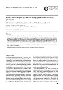
The feedforward model displays excellent results on all four events tested. Table 6 presents these specific results. These results show that the feed-forward model is able to provide sufficiently accurate forecasting for the vigicrues requirements relative to k + 1 to k + 4, i.e., for forecast lead times of 30 min to 2 h. The Nash criterion values often lie close to 0.9 and decrease as the forecast lead time increases. For the most intense event (September 2002, event no. 19), the forecasting becomes less accurate for k + 4, though the predicted Nat. Hazards Earth Syst. Sci., 12, 3307–3324, 2012

level of vigilance remains accurate. The persistence index is, generally speaking, showing that the model brings better information than a naive forecasting. On average, it is more than 0.7 and rarely under 0.5. From a temporal standpoint, in most cases examined herein, lags indicate that the forecasting is slightly late, yet the limited degradation of SPPD vs. PPD serves to mitigate this concern. While not all of the hydrographs will be presented herein, Fig. 12a and b displays the predicted hydrographs for a medium to strong event (no. 13) and the extreme event (no. 19) for the k + 3 forecast lead time (90 min). Let us note the excellent quality of forecasting for this 90-min horizon, even on an extreme event, which is higher than any event in the training set. The results are satisfactory, which often proves to be the case with this configuration, where previous discharges are inputted to the model. Moreover, positive persistence index show that the model combines discharge and rainfall in order to bring useful information. In large lead times, it can be noticed that persistency increases. This phenomenon does not mean that the forecasting is better in an absolute way, but that it is easier to work better than the naive forecast for large lead times. This observation was highlighted in Kong A Siou et al. (2011). 3.5.2

Recurrent model

The recurrent model was run in a first step with real rainfall data (as measured by the rain gauges without correction) and in a second step with a 20-set range of modified rainfall data, thus, yielding 20 discharge forecasting, in order to enhance results. These results are presented in the current section. Deterministic rainfall: The recurrent model run with observed rainfall data produced the results shown in Table 6. As expected, this model yields poorer results than the feedforward model, which takes advantage of the measured discharges as state variables. As underscored by the results presented in this section, discharge information is quite important for the model; though the recurrent model is typically capable of providing reliable alternative forecasting when discharge measurement problems occur during floods (damaged devices, transmission problems, etc.). The persistence criteria are better for intense and simple events and, as previously, for large lead times. Generally speaking, roughly 70 % of the peak discharge is accurately predicted, in many instances in terms of time as well (to within 30 min). The level of underestimation ranges from −41 % to −17 % relative to SPPD, with an average of −30 % and a standard deviation of 8 %. Despite this underestimation, the relative constancy could allow forecasters to adapt their decision during operational applications. For an www.nat-hazards-earth-syst-sci.net/12/3307/2012/


3319

Table 5. Main characteristics of the events selected for the test step (Qx : peak discharge, Qa : average discharge, P : average rainfall during the event and Ix : maximum observed hourly intensity). No.

Date

13 19 8 302

Sep 2000 Sep 2002 Nov 1996 Nov 2003

Peaks

Qx (m3 s−1 )

Qa (m3 s−1 )

P (mm)

Ix (mm h−1 )

1 1 2 1

454 819 269 200

70 116 47 67

230 235 222 155

40 82 26 16

Table 6. Results obtained by the feedforward model (Vp : level of vigilance predicted by the model, Vo : level of vigilance required given the observed discharge, Lag: delay between the maximum observed discharge and maximum forecast discharge). Event

l (0.5 h)

R2

Cp

PPD

SPPD

Vp

Vo

Lag (0.5 h)

13 13 13 13 19 19 19 19 8 8 8 8 302 302 302 302

1 2 3 4 1 2 3 4 1 2 3 4 1 2 3 4

0.99 0.98 0.97 0.95 0.93 0.94 0.94 0.78 0.97 0.94 0.91 0.88 0.97 0.95 0.93 0.89

0.73 0.92 0.96 0.95 0.42 0.65 0.7 0.67 0.64 0.75 0.67 0.70 0.65 0.8 0.84 0.79

98 % 96 % 96 % 95 % 86 % 89 % 94 % 87 % 99 % 90 % 88 % 83 % 91 % 87 % 83 % 81 %

94 % 95 % 88 % 94 % 71 % 89 % 94 % 82 % 99 % 85 % 79 % 77 % 88 % 82 % 82 % 76 %

O O O O R R R R Y Y Y Y Y Y Y Y


1 1 1 1 −1 0 0 1 0 1 1 1 2 1 2 1

0.93 0.05

0.74 0.14

90 % 6%

86 % 8%

– –

– –

0.81 0.8

Average Std. Dev.

average event, the synchronization of peaks is better than that obtained by use of the feedforward model. Here once again, we will not present all of the hydrographs produced, but limit our display to the following ones: event no. 8 for k + 1, no. 13 for k + 2, no. 302 for k + 3, and no. 19 (the most intense of the entire database) for k + 4 (Fig. 10). The event 8 shows a good consideration of the hydrological dynamics by the model. Particularly, it is worth noting that the increase of discharge at the beginning of the peaks is anticipated by the model. However, the second peak is slightly underestimated. Even with a little underestimation, the event 13 is well forecast in any case. Its standard shape can be easily linked to the shape of the rainfall signal so that the model, trained on intense and “impulse shaped” events, responds well. The event 302 is the most underestimated, at any instant of the event. Here again, the model reproduces well the general dynamics of the event, but the lack of amplitude is important. Finally, the forecasting on event 19 is of excellent quality especially when recognising that it is the most intense event of the database (roughly two times greater


than the second most intense event) and when recalling that this event, as a test event, was not used in either the training or stopping sets. Such a result proves that neural networks, if used with rigorous regularisation methods, can generalise efficiently to extreme never encountered events. Surprisingly (except for persistence), it can be observed on few events that performances tend to stabilise, or sometimes slightly increase, when the lead time increases. In order to confirm this observation over larger dataset, the crosscorrelation score is shown in Table 8 for the various lead times. One can note that this score is slightly better for k + 1, invalidating thus the previous observation in a general way. One can also note that the cross-validation score actually stabilises from k + 2 to k + 4 lead times. The last point would suggest that the recurrent model would actually be able to anticipate short term future rainfalls. Ensemble forecasting: In order to further enhance the results obtained, the uncertainty in rainfall measurements has been considered by Nat. Hazards Earth Syst. Sci., 12, 3307–3324, 2012

3320


Fig. 8. (a) Predicted and observed hydrographs for the k+3 horizon on event no. 19 using the feedforward model; (b) predicted and observed hydrographs for k + 3 horizon on event no. 13 with the feedforward model.

Fig. 9. Forecast and observed discharges for the four tested events with the recurrent model (the forecast lead times are indicated).

introducing a random component in the rainfall values. Future rainfall data were no longer applied to the model. The two main sources of uncertainty are: (i) the rain gauge itself and its location; and (ii) the spatial variability of both rainfall (especially relative to convective rainfall, which is the case within the Cévennes range) and strong winds. In this study, these uncertainties have been estimated at around 20 %, which is consistent with the conclusions by Marchandise (2007).


Consequently, a random modification of the rainfall was performed: each test set value used was multiplied by a random number between 0.8 and 1.2. This process was repeated 20 times, providing 20 different rainfall inputs for the model. No bias was introduced due to the poor knowledge of the rainfall field on the eastern part of the basin, combined with the high rainfall heterogeneity. In order to compare the results obtained using this model with the deterministic forecasting from Sect. 4.5.2., and as the most representative criterion for our purpose, SPPD was



3321

Table 7. Results output by the recurrent model (Vp : level of vigilance predicted by the model, Vo : vigilance required given the observed discharge, Lag: delay between the maximum observed discharge and maximum predicted discharge). Event

l (0.5 h)

R2

Cp

PPD

SPPD

Vp

Vo

Lag (0.5 h)

13 13 13 13 19 19 19 19 8 8 8 8 302 302 302 302

1 2 3 4 1 2 3 4 1 2 3 4 1 2 3 4

0.94 0.95 0.93 0.93 0.85 0.92 0.91 0.91 0.8 0.78 0.77 0.81 0.63 0.64 0.57 0.57

0.07 0.65 0.82 0.86 −0.25 0.71 0.84 0.89 −4.52 −0.84 0.33 0.15 −13.3 −3.51 −2.31 −0.63

84 % 83 % 79 % 77 % 67 % 72 % 74 % 83 % 70 % 62 % 67 % 65 % 64 % 70 % 72 % 65 %

81 % 79 % 79 % 75 % 63 % 69 % 73 % 83 % 70 % 62 % 63 % 59 % 64 % 70 % 72 % 63 %

O O Y Y O O R R Y Y Y Y Y Y Y Y


1 1 1 1 −1 −1 −1 0 0 0 1 2 0 1 0 1

0.81 0.14

−1.25 3.61

72 % 7%

70 % 8%

– –

– –

0.38 0.81

Average Std. Dev.

Table 8. Evolution of the cross-validation score versus the forecast lead-time. Lead time Cross validation score (0.10−6 )

Fig. 10. Summary of results obtained from ensemble forecasting compared with deterministic forecasting output.

chosen as the descriptive parameter. Figure 10 presents the maximum, minimum and average SPPD values derived from the ensemble forecasting, along with the SPPD values output by deterministic rainfall forecasting.


1

2

3

4

161

174

175

179

We have demonstrated herein that no improvement is gained by this method. The average results of ensemble forecasting are, as a general rule, either nearly the same or worse than the output of deterministic forecasting. The lag results, which have not been presented herein, also turn out to be similar. The maximum values can yield excellent results, yet in real-time use this information proves irrelevant. As a matter of fact, the question surrounding the choice of leading ensemble remains unsolved for the forecaster. It is currently recognised that when the average ensemble forecasting is similar to the deterministic forecasting, then the contribution of the ensemble forecasting becomes quite limited. Nevertheless, this part of the study has sparked discussion about the robustness of the recurrent model. Generally speaking, events nos. 8 and 302 display a lower variability than the others. We analysed this result through a diminished impact of rainfall modification on lower intensities and cumulative rainfalls. In the case of low-intensity events, the model shows relative insensitivity to rainfall uncertainty. In the case of higher-intensity events, the conclusion is rather ambiguous, but with the exception of maximum and minimum values, a low dispersion can be noticed. The model used, therefore, shows limited sensitivity to noise in the test set input data. Nat. Hazards Earth Syst. Sci., 12, 3307–3324, 2012

3322


If no strict forecasting enhancement is obtained, then model robustness is assessed and can be qualified as reasonable.

4

Discussions

The results obtained prove again the neural networks ability to provide robust and efficient forecasting in complex nonlinear natural systems. Here is targeted a small basin regularly submitted to flash floods. Previous work in the area was made by Toukourou et al. (2009, 2011) on the Gardon d’Anduze basin (545 km2 ). This basin is bigger than the Gardon de Mialet and not as homogeneous as the Gardon de Mialet basin is, even if they are nested. Consequently, the Gardon d’Anduze behaviour is more complex with lots of sub-basins, high slopes differences, geological heterogeneity... Thus, the maximum forecast lead time can be of the same order in both basins because the Gardon d’Anduze may be more sensitive to rainfall location, thereby reducing the average visibility. For these reasons, it would probably be difficult to build an efficient recurrent model for Anduze. We showed, in the present study, that for a simple basin, a linear part combined to a nonlinear one in the model brings a significant enhancing to a MLP feedforward model. This behaviour may be linked to the basin behaviour. The transformation of rainfall into discharge is more direct for rapid basin: both signals (average rainfall and discharge) have the same shape so that a linear relation can bring enhancement to the modelling process, while the nonlinear part supports complex relations. Concerning the shorter lead time k +1, forecasts are sometimes worse on the intense events chosen compared to the other events. One can explain this lower quality by the hydrologic behaviour of the basin and by the bias variance tradeoff. In order to explain this, we should observe Dolciné et al. (2001) work on the Gardon d’Anduze basin. They show that, very short-term rainfall forecast is not necessary to provide accurate discharge forecasting. Even if in the present work, no rainfall forecasting is used, the underlying phenomenon is the same. In both cases, the last rainfall values (forecast or observed) provided to the model are not useful to explain the short-term estimated discharge. Indeed, the rainfall recently observed (one or two step times before the instant of forecasting) is not yet participating to the hydrological response. In our study, this means that some recent values are unnecessary for short forecast lead times while they are still provided to the model. They increase complexity by increasing the number of parameters; taking into account the bias-variance tradeoff, this may degrade the forecasts obtained. A point is common amongst all of the studies about neural network hydrological modelling: a rigorous application of regularisation methods is a reliable path to design a wellworking neural network model. Then, if data are available, Nat. Hazards Earth Syst. Sci., 12, 3307–3324, 2012

the use of previous measured discharges is recommended for short-term forecasting; for longer terms forecasting it would be useful to take profit of the recurrent model, which seems to grasp the dynamics of the basin better. Finally, ensemble predictions do not enhance the results obtained by the recurrent model. The advantage is very clear: the sensitivity of the model to rainfall uncertainty is low. On the other hand, no improvement is obtained. In these conditions, if a bias could have been defined (under or overestimating of the rain gauges), we could have been opening another path of inquiry, in which forecasting could have been enhanced considering better the reliability of the rainfall measurements.

5

Conclusions

The potential human and financial losses related to flash floods have made their study and forecasting a very challenging concern. In this paper, we have evaluated six types of models based on machine learning: the first category belongs to feedforward models using previous observed discharge values, while the second represents recurrent models using previous estimated discharge values. In each category, linear, classical MLP and combined linear and MLP models were assessed, each one type was set forth in four versions corresponding to four forecast lead times. It appeared then that combined models were superior to the others and provided very good forecasts up to the response time of the basin without any assumption about future rainfalls. End users can benefit from these results in order to decrease the uncertainty inherent to flash flood forecasting. A rigorous variable selection process (using basin response times) and an accurate application of regularisation methods (early stopping, cross-validation) have highlighted the ability of neural networks to model nonlinear recurrent systems such as rapid basins. Their parsimony is highly valued in the context of flash flood forecasting, as characterised by a poorly known hydrological context, missing data and partial data unavailability during real-time use. As exhibited in the literature, the feedforward model is the more efficient. Applied to the Mialet Basin, it yields efficient forecasting on any kind of event tested up to a 2-h horizon. In the case of data transmission difficulties or discharge gauge damage, the recurrent model outputs forecasting in a degraded mode. Though efficiency is lower, still in most instances 70 % of the peak discharge is predicted. In order to raise this ratio value, ensemble forecasting that take into account the great uncertainty on rainfall inputs were developed. Unfortunately, the average results of these forecasting were nearly equal to those obtained using the simple input version. The longer computation time these forecasting require is not justified by the improvement in results. Nevertheless, the low sensitivity of neural networks to the noise and inaccuracy found in the test set has been demonstrated. This www.nat-hazards-earth-syst-sci.net/12/3307/2012/

G. Artigue et al.: Flash flood forecasting in poorly gauged basins using neural networks property constitutes another advantage of the neural network approach. It can be highlighted that such conclusions are generic and can be applied to any other basin in which data would be available for a sufficient number of events. Next, by taking soil moisture into account using associated indices or previous long-term rainfall series, the model could be enhanced, especially when considering the great seasonal variations in initial conditions. Lastly, after enhancing these forecasting, a generalisation of recurrent model forecasting to ungauged basins remains the main purpose of our future research.

Acknowledgements. The authors would like to thank SCHAPI for the availability of their BVNE project, with special mention of Caroline Wittwer and Arthur Marchandise for supplying data and hosting constructive discussions on flash flood forecasting. Sincere thanks are also addressed to the Hydrosciences Montpellier and Centre des Matériaux de Grande Diffusion research teams. Our gratitude is extended to the Civil Engineering student body of the Ecole des Mines d’Alès School, particularly Guillaume Burg and Pierre Etchart whose work has contributed to these research projects. The constant efforts made by Dominique Bertin (with the Geonosis Company) to enhance and develop the neural network software RNF Pro are hereby acknowledged as well. And lastly, special thanks go to the French National Research Agency for its support of the FLASH project (ANR-09-SYSC 004), which has contributed to the present work. Edited by: N. R. Dalezios Reviewed by: two anonymous referees

References Alfieri, L., Smith, P. J., Thielen-del Pozo, J., and Beven, K. J.: A staggered approach to flash flood forecasting – case study in the Cévennes region, Adv. Geosci., 29, 13–20, doi:10.5194/adgeo29-13-2011, 2011. Artigue, G., Johannet, A., Borrell, V., and Pistre, S.: Flash floods forecasting without rainfalls forecasts by recurrent neural networks, Case study on the Mialet basin (Southern France), Proceedings of the 3rd world congress on Nature and Biologically Inspired Comuting, 19–21 Oct. 2011 in Salamanca, 303–310, 2011. Ayral, P. A.: Contribution a` la spatialisation du modèle opérationnel de prévision des crues e´ clair ALHTAÏR, approches spatiale et expérimentale, application au bassin-versant du Gardon d’Anduze, PhD Thesis, Université de Provence, 311 pp., 2005. Barron, A. R.: universal approximation bounds for superpositions of a sigmoidal function, IEEE Transactions on Information Theory IT-39, 930–945, 1993. Bartholmes, H. and Todini, E.: Coupling meteorological and hydrological models for flood forecasting, Hydrol. Earth Syst. Sci., 9, 333–346, doi:10.5194/hess-9-333-2005, 2005. Beven, K. J. and Kirkby, M. J.: A physically based variable contributing area model of basin hydrology, Hydrol. Sci. Bull., 24, 43–69, 1979.


3323

Beven, K. J., Quinn, P., Romanivicz, R., Freer, J., and Lamb, R.: TOPMODEL, in: Computer models of watershed hydrology, edited by: Singh, V .P., Water Resources Publications, Highlands Ranchs, Colo., 627–668, 1995. Borrell, V., Chorda, J., and Dartus, D.: Prévision des crues e´ clair, C. R. Geoscience, 337, 1109–1119, 2005. Ceresetti, D.: Structure spatio-temporelle des fortes précipitations : application a` la région Cévennes-Vivarais, PhD Thesis, Université de Grenoble, Laboratoire d’étude des Transferts en Hydrologie et Environnement, 283 pp., 2011. Corzo, G. and Solomatine, D.: Knowledge-based modularization and global optimisation of artificial neural network models in hydrological forecasting, Neural Networks, 20, 528–536, 2007. Coulibaly, P., Anctil, F., and Bobee, B.: Daily reservoir inflow forecasting using artificial neural networks with stopped training approach, J. Hydrol., 230, 244–257, 2000. Coustau, M., Ricci, S., Borrell, V., Piacentini, A., Thual, O., Bouvier, C., and Marchandise, A.: Calibration of rainfall runoff hydrological model for flash flood forecasting using data assimilation, EGU, poster, European Geosciences Union General Assembly 2011 Vienna, Austria 3–8 April 2011, 2011. Dolciné, L., Andrieu, H., Sempere-Torres, D., and Creutin, D.: Flash flood forecasting with coupled precipitation model in mountainous Mediterranean basin, J. Hydrol. Eng., 6, 1–10, 2001. Dreyfus, G.: Neural networks, methodology and applications, Springer, Berlin, 2005. Gaume, E.: Eléments d’analyse sur les crues e´ clair, PhD Thesis, Ecole Nationale du Génie Rural, des Eaux et Forêts and Institut National de la Recherche Scientifique, 359 pp., 2002. Gaume, E., Bain, V., Bernardara, P., Newinger, O., Barbuc, M., Bateman, A., Blaˇskoviòvá, L., Bloschl, G., Borga, M., Dumitrescu, A., Daliakopoulos, I., Garcia, J., Irimescu, A., Kohnova, S., Koutroulis, A., Marchi, L., Matreata, S., Medina, V., Preciso, E., Sempere-Torres, D., Stancalie, G., Szolgay, J., Tsanis, I., Velasco, D., and Viglione, A.: A compilation of data on European flash floods, J. Hydrol., 367, 70–78, 2009. Geman, S., Bienenstock, E., and Doursat, R.: Neural networks and the bias/variance dilemma, Neural Comput., 4, 1–58, 1992. Hornik, K., Stinchcombe, M., and White, H.: Multilayer Feedforward Networks Are Universal Approximators, Neural Networks, 2, 359–366, 1989. Johannet, A.: Artificial Neural Networks, Environmental hydraulics 2, Mathematical Models, 419–443, 2010. Kessler, J. and Chambraud, A.: Météo de la France, tous les climats localité par localité, J.C. Lattès, 391 pp., 1990. Kitadinis, P. K. and Bras, R.: Real time forecasting with a conceptual hydrologic model, applications and results, Water Resour. Re., 16, 1034–1044, 1980. Kong A Siou, L., Johannet, A., Borrell, V., and Pistre, S.: Complexity selection of a neural network model for karst flood forecasting: The case of the Lez Basin (southern France), J. Hydrol., 403, 367–380, 2011. Kong A Siou, L., Johannet, A., Borrell, V., and Pistre, S.: Optimization of the generalisation capability for rainfall-runoff modelling by neural networks: the case of the Lez aquifer (southern France), Environ. Earth Sci., 65, 2365–2375, 2012. Le-Lay, M. and Saulnier, G. M.: Exploring the signature of climate and landscape spatial variabilities in flash flood events: case of


3324


the 8–9 September 2002 Cévennes-Vivarais catastrophic event, Geophys. Res. Lett., 34, L13401, doi:10.1029/2007GL029746, 2007. Maier, H. R. and Dandy, G. C.: Neural networks for the forecasting and forecasting of water resources variables: a review of modelling issues and applications, Environ. Model. Softw., 15, 101– 124, 2000. Marchandise, A.: Modélisation hydrologique distribuée sur le Gardon d’Anduze: e´ tude comparative de différents modèles pluie-débit, extrapolation de la normale a` l’extrême et tests d’hypothèses sur le processus hydrologiques, PhD Thesis, Université des Sciences et Techniques du Languedoc (Montpellier), 2007. Météo France, Jacq, F.: Pluies Extrêmes en France Métropolitaine, availanle at: http://pluiesextremes.meteo.fr/index.php, last access: 28 July 2011. MEDDTL, Ministère de l’Ecologie, du Développement Durable, des Transports et du Logement, available at: http://www. vigicrues.gouv.fr (last access: October 2012), 2011. Moussa, R., Chahinian, N., and Bocquillon, C.: Distributed hydrological modelling of a Mediterranean mountainous catchment – model construction and multi-site validation, J. Hydrol., 337, 35– 51, 2007. Nash, J. E. and Sutcliffe, J. V.: River flow forecasting through concepteual models part I – A discussion of principles, J. Hydrol., 10, 282–290, 1970. Pereira Filho, A. J. and Dos Santos, C. C.: Modeling a densely urbanized watershed with an artificial neural network, weather radar and telemetric data, J. Hydrol., 317, 31–48, 2006. Piotrowski, A., Napiórkowski, J. J., and Rowiński, P. M.: Flashflood forecasting by means of neural networks and nearest neighbour approach – a comparative study, Nonlin. Processes Geophys., 13, 443–448, doi:10.5194/npg-13-443-2006, 2006. Préfecture du Gard: Direction Départementale de l’Equipement, Règlement de surveillance, de prévision et de transmission de l’information sur les crues, availhttp://www.gard.equipement.gouv.fr/IMG/pdf/ able at: RIC SPCGD version 2011 cle7bd5c2.pdf (last access: October 2012), 2006. Rouzeau, M., Martin, X., and Pauc, J. C.: Retour d’expérience des inondations survenues dans le département du Var les 15 et 16 Juin 2010, Rapport du Ministère de l’Ecologie, de l’Energie, du Développement Durable et de la Mer, en Charge des Technologies Vertes et des Négociations sur le Climat, Ministère de l’Intérieur, de l’Outre-Mer et des Collectivités Territoriales, Secrétariat d’Etat Chargé de l’Ecologie, Inspection générale de l’Administration, Conseil Général de l’Environnement et du Développement Durable, 87 pp., 2010.


Sahoo, G. B., Ray, C., and De Carlo, E. H.: Use of neural network to predict flash flood and attendant water qualities of a mountainous stream on Oahu, Hawaii, J. Hydrol., 317, 63–80, 2006. Schmitz, G. H. and Cullmann, J.: PAI-OFF: A new proposal for online flood forecasting in flash flood prone catchments, J. Hydrol., 360, 1–14, 2008. Sjöberg, J. and Ljung, L.: Overtraining, regularisation and searching for minimum in neural networks, Preprint IFAC Symposium on Adaptive Systems in Control and Signal Processing, 1992. Stone, M.: Cross-validatory choice and assessment of statistical forecasting, J. Roy. Stat. Soc., B36, 111–147, 1974. Sudheer, K. P., Gosain, A. K., Rangan, D. M., and Saheb, S. M.: Modelling evaporation using an artificial neural network algorithm, Hydrol. Process., 16, 3189–3202, 2002. Sun, X., Mein, R. G., Keenan, T. D., and Elliott, J. F.: Flood estimation using radar and raingauge data, J. Hydrol., 239, 4–18, 2000. Tabary, P., Dupuy, P., L’Henaff, G., Laurantin, O., Merlier, C., and Soubeyroux, J. M.: A 10-year (1997–2006) reanalysis of quantitative precipitation estimation over France: methodology and first results, Hydrol. Sci. J., in press, 2012. Toukourou, M. S., Johannet, A., and Dreyfus, G.: Flash flood forecasting by statistical larning in the absence of rainfall forecast: a case study, Engineering Applications of Neural Networks Proceedings, 98–107, 2009. Toukourou, M., Johannet, A., Dreyfus, G., and Ayral, P.-A.: Rainfall-runoff modelling of flash floods in the absence of rainfall forecasts: the case of “Cévenol flash floods”, J. Appl. Intell., 35, 1078–189, 2011. Tramblay, Y., Bouvier, C., Martin,C., Didon-Lescot, J. F., Todorovik, D., and Domergue, J. M.: Assessment of initial soil moisture conditions for event-based rainfall-runoff modelling, J. Hydrol., 387, 176–187, 2010. Vinet, F.: Geographical analysis of damage due to flash floods in southern France: The cases of 12–13 November 1999 and 8–9 September 2002, Appl. Geogr., 28, 323–336, 2008. Younis, J., Anquetin, S., and Thielen, J.: The benefit of highresolution operational weather forecasts for flash flood warning, Hydrol. Earth Syst. Sci., 12, 1039–1051, doi:10.5194/hess-121039-2008, 2008.


Flash flood forecasting in poorly gauged basins using neural networks ...

Flash flood forecasting in poorly gauged basins using neural networks ...

Suggest Documents

Operational river discharge forecasting in poorly gauged basins: the ...

Neural networks-based operational prototype for flash flood forecasting

Water predictions in poorly gauged basins: set-up and ...

Neural Networks in Business Forecasting

Forecasting Financial Markets Using Neural Networks

time series forecasting using neural networks - arXiv.org

Forecasting Energy Commodity Prices Using Neural Networks

Multi-step-ahead neural networks for flood forecasting - CiteSeerX

Flood forecasting using medium-range

Performance of neural networks in forecasting daily precipitation using ...

Quantitative Flood Forecasting on Small- and Medium-Sized Basins: A ...

Flash Flood/Flood Safety

Understanding sources of uncertainty in flash-flood forecasting for ...

Neural Networks in Business Forecasting

Internet Traffic Forecasting using Neural Networks - Semantic Scholar

Inflow forecasting using Artificial Neural Networks for reservoir operation

Hydrologic forecasting using artificial neural networks: a ... - CHRS - UCI

Building Energy Load Forecasting using Deep Neural Networks

Forecasting of Chaotic Time Series Using RBF Neural Networks

Forecasting and Analysis of Marketing Data Using Neural Networks

peak weather forecasting using feedforward neural networks - CiteSeerX

Using Recurrent Neural Networks To Forecasting of Forex

Short Term Load Forecasting Using Neural Networks and Particle ...

Forecasting of Chaotic Time Series Using RBF Neural Networks ...