Flexible and Efficient Querying and Ranking on Hyperlinked Data Sources Ramakrishna Varadarajan, Vagelis Hristidis School of Computing & Information Sciences Florida International University Miami, FL 33199
{ramakrishna,vagelis}@cis.fiu.edu
Louiqa Raschid Department of Computer Science University of Maryland College Park, MD 20742
[email protected]
ABSTRACT There has been an explosion of hyperlinked data in many domains, e.g., the biological Web. Expressive query languages and effective ranking techniques are required to convert this data into browsable knowledge. We propose the Graph Information Discovery (GID) framework to support sophisticated user queries on a rich web of annotated and hyperlinked data entries, where query answers need to be ranked in terms of some customized ranking criteria, e.g., PageRank or ObjectRank. GID has a data model that includes a schema graph and a data graph, and an intuitive query interface. The GID framework allows users to easily formulate queries consisting of sequences of hard filters (selection predicates) and soft filters (ranking criteria); it can also be combined with other specialized graph query languages to enhance their ranking capabilities. GID queries have a well-defined semantics and are implemented by a set of physical operators, each of which produces a ranked result graph. We discuss rewriting opportunities to provide an efficient evaluation of GID queries. Soft filters are a key feature of GID and they are implemented using authority flow ranking techniques; these are query dependent rankings and are expensive to compute at runtime. We present approximate optimization techniques for GID soft filter queries based on the properties of random walks, and using novel path-length-bound and graphsampling approximation techniques. We experimentally validate our optimization techniques on large biological and bibliographic datasets. Our techniques can produce high quality (Top K) answers with a savings of up to an order of magnitude, in comparison to the evaluation time for the exact solution.
Categories and Subject Descriptors H.3.3 [Information Search and Retrieval]
General Terms Algorithms, Performance, Experimentation.
Keywords soft filters, hard filters, authority flow ranking, ObjectRank.
1. INTRODUCTION Consider a rich web of annotated data entries (objects) in Internet accessible sources with hyperlinks to entries in other Permission to copy without fee all or part of this material is granted provided that the copies are not made or distributed for direct commercial advantage, the ACM copyright notice and the title of the publication and its date appear, and notice is given that copying is by permission of the ACM. To copy otherwise, or to republish, to post on servers or to redistribute to lists, requires a fee and/or special permissions from the publisher, ACM. EDBT’09, March 24–26, 2008, Saint Petersburg, Russia. Copyright 2009 ACM 978-1-60558-422-5/09/0003 ...$5.00.
Maria-Esther Vidal, Luis Ibáñez, Héctor RodríguezDrumond Department of Computer Science Universidad Simón Bolívar Caracas, Venezuela {mvidal,ldibanyez,hector}@ldc.usb.ve
sources. Examples include the biological Web, GIS datasets and their metadata, bibliographic data sources, healthcare data, desktop files and Intranets. Such graphs have significant differences from the general Web graph. Each of the data entries or documents contains some specific typed knowledge, e.g., information on genes and proteins for the biological Web. Thus, this graph has an underlying schema graph. Users of such typed webs want answers to queries that are meaningful to them and go beyond traditional Information Retrieval (IR) keyword queries. These users have sophisticated information needs, which require both customization and personalization, when ranking query results. For example, a biologist may only want to retrieve protein data entries from SwissProt, or she may be interested in discovering the associations between a particular drug and a disease by following the links among publications that are linked to proteins and vice versa.. The challenges to query answering in this rich web of entities include supporting users to retrieve meaningful answers, given the user’s preferences, rather than just retrieving relevant data entries. The Graph Information Discovery (GID) framework must support a simple yet flexible query interface where a user can easily pose a complex query. Ranking of answers must reflect the semantics of this rich Web and the user’s personal perspective. GID queries must be interactive and support the exploratory discovery process. Hence, they must support formal semantics so that queries can be optimized and evaluated efficiently. The limitations of many prior solutions are that they typically converge on the extremes of query complexity, i.e., plain keyword or complex queries, with few solutions in between, or they fail to consider ranking. Web search [11, 12, 14, 22, 23] employs excellent ranking techniques but have limited search capability. The keyword search paradigm of Web search has also been adapted to structured databases [3, 5, 6, 16, 29]. On the other hand, there are a variety of extensions of SQL for Web graphs (WebSQL [21], W3QL [20], WebOQL [4], StruQL[12]) and RDF graphs (SPARQL [28]). However, none of these languages provide customized ranking techniques. The approach in [24] is an excellent start towards incorporating ranking in structured Web queries. They provide an underlying algebra and optimization; however, they do not support an interface that allows users (scientists in the case of the scientific Web) to intuitively write useful complex queries, nor do they support powerful ranking techniques like authority flow based ranking. NAGA [19] implements reasoning tasks on RDFS documents, and supports complex queries and ranking. NAGA targets typed graphs of facts and labeled relationships that may be expensive to create and keep up-to-date. It does not support query-customized ranking. That is, a fixed confidence-based ranking function is applied to the final results. In contrast, GID allows the user to specify what ranking
Figure. 1 Sample Data Graph for a Biological Dataset. mechanism (if any) should be used for each leg of the query. Furthermore, NAGA uses expensive reasoning algorithms, which may not scale to very large datasets like PubMed, whereas GID relies on a suite of scalable approximation and optimization techniques. We show in Section 4 that our framework can complement such prior research and extend it with support for sophisticated queries and ranking. This paper addresses the challenges of expressing and answering sophisticated user queries on typed graphs. We focus on a web of annotated data entries from biological data sources for our running examples and experiments. However, the generic GID framework is applicable in multiple domains; we use bibliographic data as a second evaluation domain in our experiments. The GID framework has the following features and capabilities: •
Given a typed graph, GID provides a user interface to specify a combination of hard and soft filters; the latter incorporate ranking in an intuitive manner. GID emulates domain graph query languages such as lgOR, lgPR [25] and filter queries in PubMed [1]. GID can be combined with more general graph languages to support complex queries.
•
Filters are implemented by an underlying closed algebra of physical operators. Each operator produces a ranked graph and GID operators can be combined. The properties of the operators are used to determine the relevant query rewriting rules.
•
GID soft filters are implemented using authority flow based ranking; they are query dependent and must be computed at runtime. Two novel approximation techniques are studied in order to achieve interactive query response times. One is a path-length-bound technique, where only paths of limited length are considered. The second is a graph-sampling approximation technique, where sampling over a Bayesian network is used to create sampled graphs and estimate the ranking scores.
•
GID queries were evaluated on biological and bibliographic datasets. We show that our approximation methods achieve execution time reductions of up to an order of magnitude, with negligible degradation of the Top-k answer’s quality (in comparison to the exact ranking). This allows GID to support an exploratory framework.
The paper is organized as follows: Section 2 presents the data model. Section 3 describes the query language. Section 4
presents related work. Section 5 presents the algebra and Section 6 discusses authority flow techniques used to implement soft filters and their efficient evaluation. Section 7 presents the GID optimizer and its execution. Section 8 presents the quality and performance experiments. Finally, Section 9 presents our conclusions and future work.
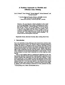
2. DATA MODEL The GID framework views a database as a labeled graph; this captures both relational and XML databases. It includes a data and a schema graph. The data graph DG(VD,ED) is a labeled directed graph where every node (object) v has a type λ(v), a set A1,…,As of attributes with attribute values A1(v),…,As(v) and a set c(v) of keywords. For example, the node “PMID 14656967” of Figure 1 has type “PubMed” and attributes “Title” and “Authors” and the set of keywords includes {“mammals”, “histocompatibility”, …}. The schema graph SG(VS, ES) (Figure 2) is a directed graph that describes the structure of a data graph DG. Every node v and every edge e have an associated type λ(v) or λ(e), respectively. For instance, the “Entrez Gene” to “PubMed” edge in Figure 2 has type “GN-PM”. We say that a data graph DG(VD,ED) conforms to a schema graph SG(VS,ES) if there is a unique assignment µ of data-graph nodes to schema-graph nodes and a consistent assignment of edges as follows: 1. for each v ∈ VD there is a µ(v) ∈ VS such that λ(v)=λ(µ(v)); 2. for every edge e ∈ ED from node u to node v there is an edge µ(e) ∈ ES that goes from µ(u) to µ(v) and λ(e) = λ(µ(e)).
Figure. 2 Subset of Schema Graph for a Biological Dataset.
3. GID QUERY LANGUAGE The intuition of the GID framework is the application of a sequence of hard and soft filters. A filter generally takes as input a ranked graph and outputs a ranked subgraph of the input graph. A hard filter is used to eliminate some nodes in a Boolean manner whereas a soft filter provides ranking.
3.1 GID Query Syntax Given a data graph DG and a schema graph SG, a query q is a sequence q=[r1>…>rm] of filters ri. We use the “>” symbol to denote a total order between the filters and this represents a pipelining of the output of one filter as input to the next. The results of a query, which are usually (see exception below) the nodes of the graph output by the last filter, are referred to as target objects. A query may also specify the number k of the requested top-k results. A filter r={R,N,S} is the following 3tuple: (1) The selection condition R as follows: • • • •
A keywords Boolean (OR, AND, NOT) expression E, e.g., Keywords = “cancer” AND “breast”. An attribute value pair av, e.g., title = “A comparative…” A type T, e.g., Type = {EntrezGene}. A Path expression P, e.g., Path = EntrezGene /PubMed or Path = EntrezGene [Keywords = “tnf”] / PubMed [author=“Michael”].
(2) A Boolean N; the value=true means that r is negated. (3) A Boolean S; a value=true means that r is soft. GID does not support soft filters (S=true), where R is a path expression, or negated soft filters (N=true and S=true) since the semantics are unintuitive. Path expression P may contain types, unidirectional single step navigational operators (/), multi-step navigational operators (//), and type wildcards (*). Notice that “Path”, “Keywords” and “Type” are reserved words in GID. GID does not support a combination of selection conditions (keyword expression, attribute value pair, type or path expression) within a single filter, in order to simplify the implementation and optimization process. Example 1: A biologist’s exploration is as follows: Starting from genes in Entrez Gene she follows links to Entrez Protein and then to PubMed; her target objects are a set of papers in PubMed. She wants to rank these papers by their importance/relevance to the word “human”. The following expresses her needs:
$EntrezGene$/EntrezProtein, false, false}] returns all EntrezGene objects that point to an EntrezProtein object.
3.2 GID Query Semantics To define the semantics of GID queries, we first define a score assignment function, Score for a data graph DG(VD,ED) to be a mapping of nodes v∈VD to real values Score(v) in [0,1]. A unit score assignment, Scoreunit, assigns Scoreunit(v)=1 to every v∈VD. The input of a filter r is a pair (Gin,Scorein) of a data graph Gin and a scores assignment Scorein for Gin. Similarly, the output is a pair (Gout,Scoreout), where Gout is a subgraph of Gin. Applying the filter is as follows: r(Gin,Scorein)=(Gout,Scoreout). Given a GID query q=[r1>r2>…>rm-1>rm] on the data graph DG=(VD,ED) the result (GR,ScoreR) of q is rm(rm-1(…(r2(r1(DG, Scoreunit)))…)). During query evaluation, filters are applied in the order indicated in the query. Note that the unit score assignment is used for the first filter r1. Alternative initial scores are possible, e.g., the global score of a node computed by a method like PageRank [23]. Each filter may change the scores of the data graph. This may also eliminate nodes and edges as explained next. Applying filter r on graph DG is as follows: • •
Each v in DG is assigned a score Score(v) in [0.0,1.0]. When node v is assigned Score(v)=0, then the node and its incident edges are removed. For example, applying r = {Keywords=“human”, false, false} removes all nodes and incident edges in graph Gin that do not contain the keyword “human” to create Gout .
Given the result (DGR,ScoreR) of q, where DGR=(VR,ER), GID will display a list of the nodes v of VR ranked by decreasing ScoreR(v) values. Hard filters are used to eliminate nodes (and their incident edges) of Gin. The filter is evaluated as a Boolean and may assign score 0 to some nodes. The score is unchanged for the rest of the nodes. Consider the following filter r={R,false,false}:
q1 = [{Path = EntrezGene/EntrezProtein/PubMed, false, false} > {Keywords=“human”, false, true} > {Type = PubMed, false, false}].
1.
If R is a keyword expression E (or simply a keyword), Scoreout(v)=0 if v does not satisfy E, else Scoreout(v) = Scorein(v).
The first hard filter creates a subgraph of paths from genes in Entrez to proteins to PubMed publications. The second, soft filter provides a “goodness” ranking (to be discussed below) with respect to the keyword “human”, and the last, hard filter identifies the “target objects” - publications from PubMed – in the result.
2.
If R is a attribute value pair av, then Scoreout(v)=0 if node v does not satisfy av, else Scoreout(v) = Scorein(v).
3.
If R is a type T, then Scoreout(v)=0 if v is not of type T, else Scoreout(v)=Scorein(v).
4.
If R is a path P, then Scoreout(v)=0 for nodes not contained in a path of type P, else Scoreout(v)=Scorein(v).
The most simple and intuitive GID query for novice users is to specify a set of hard filters {r1,…,rt } and a single soft filter rs. This can have a default interpretation of q ={r1,…,rt} > rs or as q = rs >{r1,…,rt} depending on the application semantics. The specific ordering of the hard filters {r1,…,rt} is not important as long as they do not include Path filters as shown in Section 5.2. Target Objects: As mentioned above, we assume by default that all the objects of the resulting subgraph of the query are output to the user. Alternatively, the $ sign is used to select a more finegrained group of target objects. For instance, q2 = [{Path =
The opposite scores are assigned if r={R,true,false}. Soft filters rank a result subgraph and are inherently fuzzy. Suppose R is a keyword w or keyword expression E, then, applying r results in the following score: Scoreout(v)=f(Scorein(v),Scorer(v)) 0≤Scorer(v)≤1 is the score assigned to v by r. Scorer(v) shows how “good” v is, given the graph Gin. GID does not specify the exact semantics or computation of these scores Scorer(v) for soft filters. Various approaches are possible including authority flow (Section
6), IR scoring [27], path count [18], keyword proximity [13, 17], minimum distance from the keyword nodes and so on. Note that Scorer(v) must be positive (non-zero) and must not depend on the input score assignment Scorein(v). This important assumption, the non-pruning order-free assumption for soft filters, is needed to obtain useful rewriting axioms. This assumption is reasonable to implement since a small epsilon value can be assigned to nodes instead of 0 if they are completely irrelevant to R. We use a combining function f (e.g., product or min). In principle, any combining function may be used. However, a monotone function is usually more intuitive and also allows pipelining and fast computation of the top results [10]. In order to maintain the Score(v) in [0.0,1.0], we normalize the Score(v) after application of each filter. Example 1 (cont’d): Figure 3 shows the query evaluation of query q1 given the input data graph DG of Figure 1. We assume initial unit scores assignment Scoreunit. We also assume a simple soft filter scoring function with Scorer(v)=0.5 if a node does not contains the term and Scorer(v)=1 otherwise. The combining function f is summation.
4. RELATED RESEARCH Meeting target user needs: We interviewed biomedical domain experts and examined popular search tools. When asked to describe the selection of target objects (results) that are documents in PubMed, these users chose progressive filtering of the objects; see PubMed filter queries [1]. They also requested simple navigational paths. PubMed supports filters in a limited manner; users can select a set of predefined filters (hard filters in our terminology), e.g., filter the publications that cite MEDLINEplus articles. In [29], we conducted user experiments that show the benefits of soft filters for this domain. We note that the real test of the GID framework will be a friendly graphical user interface and user evaluation studies; this is included in our future work. A second aspect of user needs is the richness of the data model. The GID model is much simpler compared to RDF, yet it can capture much of the knowledge used by a scientist in the process of literature based discovery (LBD) on the Web. NAGA [19] has a similar labeled directed multi-graph data model. However, they may have significant overhead in determining the confidence of facts and relationships of the RDFS graph. A third aspect of user needs is personalized ranking. NAGA does not support query-customized ranking. That is, a fixed ranking function is applied to the final results, based on confidence-based edge weights that reflect the estimated accuracy of the extraction process and trust in the source. In contrast, GID allows the user to specify what ranking mechanism (if any) should be used for each leg of the query. GID supports authority flow based ranking and the authority weights can be personalized. This is well suited to scientists whose value for specific domain knowledge may vary depending on the task. Expressive power: GID is clearly more powerful than the current PubMed language which only supports hard filters and has no ranking capability. Research by Raghavan and Garcia-Molina [24] studies an expressive graph algebra and query operators. The GID language can support the “linear” plans of this algebra. The “tree” plans were not considered since they cannot be supported by a simple user language. While users wanted navigation, they did not
express a need for general join operations, recursion, etc. as found in [24]. GID soft filters are more general than the ranking operators in [24]. GID soft filters are evaluated against the whole input subgraph (e.g., ObjectRank) instead of just relying on the properties of each individual node as is done in [24]. This property is the key to intuitive GID user query interface. Example 2: This example shows that the GID query language allows expressing complex queries in an intuitive way; no query language was proposed in [24]. Consider the following sample query from [24]: “Generate a list of universities with whom Stanford researchers working on ‘Mobile networking’ collaborate”. A sequence of instructions corresponding to this query is presented in [24]: Let S be a weighted set consisting of all the pages in the stanford.edu domain that contain the phrase ’Mobile networking’. The weight of a page in S is equal to the normalized sum of its PageRank and text search ranks. Compute R, the set of all the “.edu” domains (except stanford. edu) to which pages in S point. For each domain in R, assign a weight equal to the sum of the weights of all the pages in S that point to that domain. List the top-10 domains in R in descending order of their weights [24]. Creating the algebraic execution plan for this query (Figure 8 of [24]) requires significant training. In contrast, the hard and soft filters of GID can express this query in the following sequential and straightforward manner: [{Keywords="",false,true}>{IRFilter("Mobile Networking"), false, true} > {Path=Webpage[URL="stanford.edu" AND Keywords = "Mobile networking"]/$Webpage[URL=".edu" AND URL ≠ "stanford.edu"]$, false, false}> {URL="stanford.edu", false, true}]. For this query, we first initialize the graph nodes with global PageRank scores (empty keywords expression in first soft filter). For computing the textrank (IRscores), we need to introduce the IR soft filter. The combining function, f is summation that adds textranks and pageranks. Notice that the last filter is a soft filter that computes the final scores for each web page and outputs the non-Stanford.edu pages in descending score order. We assume that this attribute-constrained soft filter uses the scores of the nodes in the input graph as the weights in the base set for the authority flow execution algorithm. There has been significant work on query languages for the Web and search engines ranging from keywords based languages to query languages for semi-structured data, to graph query languages; a detailed comparison is in the extended version [30]. For users who require general query language features to write complex queries, the GID operators and ranking semantics can be incorporated in a straightforward manner into a language such as SPARQL. Alternatively, more complex path expressions or other relational operators can be incorporated into the GID language. NAGA too can express complex queries and can support a powerful inference mechanism; however, this may not scale well to large graphs and an interactive discovery process.
5. ALGEBRA FOR GID We present a closed algebra where the algebraic operators have a one-to-one correspondence to the filters of Section 3. A binary Combine operator is introduced to combine scores. Each (unary) operator, with the exception of Combine, accepts as input a pair of data graph and score assignment (DG, Score) and produces the pair (DG′, Score′), where DG=(VD,ED) and
Figure. 3 Sample semantic query evaluation. DG′=(VD′,ED′). Further, VD′ ⊆ VD and ED′⊆ ED.
5.1 Operators 1.
2.
3.
4.
5.
HardExp(DG,Score,E) → (DG′,Score′) where E is a Boolean expression over keywords, such that, VD′ ={v | v ∈ VD and satisfy(v,E)}, ED′={e=(u,v) | e∈ED and u,v ∈ VD′} and the Boolean predicate satisfy(.,.) is defined by induction over E as follows: • If E is a term, satisfy(v,E)=true if v contains the term E, false otherwise. • If E=E1 Op E2, satisfy(v,E)=satisfy(v,E1) Op satisfy(v,E2). • If E = not (E1), satisfy(v,E)= not(satisfy(v,E1)). The score of each node v∈VD′ remains the same, i.e., Score′(v)=Score(v). HardAttribute(DG,Score,av) → (DG′,Score′) where av is an attribute value pair, such that, VD′ ={v | v ∈ VD and satisfy(v,av)}, ED′={e=(u,v) | e∈ED and u,v ∈ VD′} and the Boolean predicate satisfy(v,E)=true if v contains the corresponding value for the attribute specified, false otherwise. Notice that we overload the satisfy predicate. HardType(DG,Score,T)→(DG′,Score′) where T is a set of types (nodes of the schema graph), VD′ ={v | v ∈ VD and ∃ t ∈ T and v∈ t}, ED′={e=(u,v) | e ∈ ED and u,v ∈ VD′}. The score of each node v ∈ VD′ remains the same, i.e., Score′(v)=Score(v). HardPath(DG,Score,P)→(DG′,Score′) where P is a path expression, VD′ = {v | v ∈ VD and satisfyPath(v,P)}, ED′={e=(u,v) | e ∈ ED and u,v ∈ VD′}, the Boolean predicate satisfyPath(v,P) is true if v is part of a path p that satisfies P; false otherwise. The score of each node v ∈ VD′ remains the same, i.e., Score′(v)=Score(v).
•
If E=E1 OR E2, ScoreFunction(DG,E,v) = ScoreFunction(DG,E1,v)+ ScoreFunction(DG,E2,v).
•
If E=E1 AND E2, ScoreFunction(DG,E,v) = ScoreFunction(DG,E1,v) . ScoreFunction(DG,E2,v).
•
If E=not(E1), ScoreFunction(DG,E,v) ScoreFunction(DG,E1,v).
•
If E is a term w, ScoreFunction(DG,E,v) ScoreFunction(DG,w,v).
=
1
– =
Once ScoreFunction is executed, the scores Score′(v) of the nodes in DG are updated as follows: Score′(v) = ScoreFunction(DG,E,v). Note that Score′(v) is the Scorer(v) described in Section 3.2, that is, the score assigned by the soft filter. This score will then be combined with the previous nodes scores Score(v) using the Combine operator below. 6.
Combine(DG1,Score1,DG2,Score2,f) → (DG′,Score′) where f(score1,score2) is a combining function like product. For every node in the union of DG1 and DG2, Score(v) = f(Score1(v),Score2(v)). Given DG1=(VD1,ED1) and DG2=(VD2,ED2), the graph DG′= (VD′ , ED′) is defined as follows: VD′ ={v | v ∈ VD1 ∪ VD2 and Score′(v)>0.0}, ED′={e=(u,v) | e ∈ ED1 ∪ ED2 and u,v ∈ VD′}.
Example 1 (cont’d): Figure 4 shows an execution plan for query q1. We use f(.,.)=SUM(.,.) as the combining function (other combining functions are possible as explained above) and ObjectRank as the ScoreFunction . Due to space limitations we do not describe the operators to handle negation (N=true) in the filters.
SoftExp(DG, Score, E, ScoreFunction) → (DG′, Score′) where E is a Boolean expression over keywords, and ScoreFunction is a function such that, given E and DG, maps each node v to a score ScoreFunction(DG,E,v) in [0.0,1.0] ((0.0,1.0] given the non-pruning assumption for soft filters). Alternatives for ScoreFunction include ObjectRank, path count, MinDistance, keyword proximity and so on, as discussed in Section 3.2. The score for E is computed as follows: Figure. 4 Execution plan for query q1.
5.2 Axioms In this section we present the rewriting rules for GID queries, assuming any implementation for the soft filters, i.e., any definition of ScoreFunction. These rules will be applied together with the approximations (to be shown in Section 6). Consider the following theorems (without proof): Theorem 1: Let Hi, Hj be hard filters and Si, Sj be soft filters. The following properties hold: 1. The commutative property of non-path hard filters Hi > Hj ⇔ Hj > Hi. 2. The commutative property of soft filters Si > Sj ⇔ Sj > Si. 3. The idempotence property of hard filters Hi > Hi ⇔ Hi The proof is straightforward and relies on the following: The soft filters are non-pruning and always assign a non-zero score. The combining function f which combines the scores of a soft filter with the current scores is commutative (e.g., product, sum, max). Theorem 2: The rewritings of Theorem 1 can be applied to any subsequence of a query. For example, if Q = S1>H1>H2>S2 where Hi and Sj are hard and soft filters respectively, then using the commutative property of hard filters we can rewrite Q as S1>H2>H1>S2.
6. GID SOFT FILTER COMPUTED BY AUTHORITY FLOW GID soft filters will typically be the most expensive operators since the popular authority-flow based ranking techniques used by most soft filters are well known to be expensive for relatively large data graphs. PageRank [23] and ObjectRank [5], rely on pre-computing and indexing global or keyword-specific rankings. Given that the GID framework is meant to be interactive and exploratory, we aggressively optimize the evaluation of authority-flow soft filters. We first provide an overview of some ranking metrics. We then discuss two approximation techniques.
directions and not only in the direction that appears in the schema. For example, an Entrez Gene passes its authority to the PubMed paper it is associated with and vice versa. Notice however, that the authority flow in each direction (defined by the authority transfer rate) may not be the same. For example, a PubMed paper that is cited by important papers is clearly important but citing important PubMed papers does not make a paper important. In Figure 5, different rates could be assigned to different edge types to achieve personalized authority flow rankings.
Figure. 5 Authority Transfer Schema Graph for Biological Database. Authority Transfer Data Graph. Given a data graph DG(VD,ED) that conforms to an authority transfer schema graph TSG(VTS,ETS), we can derive an authority transfer data graph TDG(VTD,ETD) as follows. For every edge e = (u→v) ∈ ED, the authority transfer data graph has two edges ef = (u→v) and eb = (v→u). The edges ef and eb are annotated with authority transfer rates α(ef) and α(eb). f
Assuming that ef is of type e S , then α ( e Sf ) , if OutDeg (u ,e Sf ) > 0 f f OutDeg ( u , e ) S α (e ) = 0, if OutDeg (u , e Sf ) = 0
where,
OutDeg(u,e Sf ) is the number of outgoing edges from u, f
6.1 Authority Flow Ranking The ObjectRank score of a node v given a keyword w is the probability that a random surfer starting from a node that contains w (the base set) will be at v at a given time. Authority Transfer Schema Graph. From the schema graph SG(VS,ES), we create the authority transfer schema graph TSG(VTS,ETS) to reflect the authority flow through the edges of the graph. In particular, for each edge eS= (u→v) of ES, two authority f
of type e S . The authority transfer rate α(eb) is defined similarly. Figure 6 illustrates the authority transfer data graph that corresponds to the data graph of Figure 1 and the authority transfer schema graph of Figure 5. Each edge is annotated with its authority transfer rate. Notice that the sum of authority transfer rates of outgoing edges of node u of type µ(u) in the authority transfer data graph may be less than the sum of authority transfer rates of outgoing edges of µ(u) in the schema graph, if u does not have all types of edges.
b
transfer edges, e S = (u→v) and e S = (v→u) are created. The two edges carry the type of the schema graph edge and, in addition, each one is annotated with a (potentially different) f b authority transfer rate - α ( e S ) and α ( e S ) respectively. We say that a data graph conforms to an authority transfer schema graph if it conforms to the corresponding schema graph. The transfer rates can be determined manually by a domain expert [5] on a trial and error basis, while [29] present techniques that allow this task to be done automatically based on the user’s feedback.
Figure 5 shows the authority transfer schema graph that corresponds to the schema graph of Figure 2 (the edge types are omitted). The motivation for defining two edges for each edge of the schema graph is that authority potentially flows in both
(1)
Figure. 6 Authority transfer data graph for Biological database.
ObjectRank computation. Consider a single keyword (w) query and the authority transfer data graph TDG(VTD,ETD). A surfer starts from a node vi of the base set S(w) (nodes in VTD that contain w), and at each step she follows an edge with probability d or gets bored and jumps to a node in S(w) with probability 1 − d. The ObjectRank value of vi is the probability that at a given point in time, the surfer is at vi. The ObjectRank scores vector rQ = [rQ(v1),…,rQ(vn)]T given keyword query w, where n=|VD|, is defined as follows:
r w = dAr
w
+
(1 − d ) s | S (w) |
(2)
where A is a n × n matrix with Aij = α(e) if there is an edge e(vi → vj) in ETD and 0 otherwise, d is the damping factor which controls the base set importance and s = [s1, . .si . , sn]T is the base set vector where si is 1 if vi ∈ S(w) and 0 otherwise. [29] presents a variant of ObjectRank called ObjectRank2, where the random surfer jumps to different nodes of the base set with different probabilities, proportional to their query-specific IR score. All optimizations described below equally apply for ObjectRank and ObjectRank2. Layered Graph ObjectRank (lgOR): The class of GID queries with a hard path filter followed by a soft term filter is very useful and expressive. [25] proposed the lgOR ranking, a variant of ObjectRank, to answer such queries. These queries apply authority flow ranking on an acyclic directed layered graph produced by the hard path filter. Example 3: Consider the following GID query: [{Path = EntrezGene/EntrezProtein/$PubMed$, false, false } > {Keywords=“aging” OR “cancer”), false, true}]. First, the hard filter creates a layered graph of paths satisfying the path expression EntrezGene/EntrezProtein /PubMed (Figure 7). A layered graph is a DAG comprised of layers; each layer has data entries of one or more types, which have only edges to data entries in the next layer of the graph. The data entries in the last layer, which are returned by the query, are called the target objects. For simplicity we assume that each layer is composed of data entries of one type. Next, the soft filter executes ObjectRank on the layered graph for the keyword expression “aging” OR “cancer”. The target objects (PubMed objects) are ranked according to their ObjectRank value.
Figure. 7 Layered Graph. A key point of lgOR is that the authority flows between objects in the layered graph are only determined by the scores of the parents of each object in the previous layer of the graph, and the incoming authority transfer rates. lgOR is defined as follows: The ranking vector R of the target objects in the last layer of the
layered graph RG=(Vlg,Elg) of k layers is defined by a transition matrix Alg and an initial ranking vector Rini: R = Alg k −1 R ini = (
k −1
∏A
lg
) R ini
(3)
l =1
The transition matrix is Alg, where, αlg(e) is the authority transfer rate of edge e between nodes u and v of type U and V, respectively, in adjacent layers p and q. The OutDeg(u,V), the outdegree of node u to nodes of the type V, is limited to nodes and edges in the layered graph as follows: if e = (u → v) ∈ Elg α lg(e), Alg [u, v] = 0 , otherwise
(4)
6.2 Approximation Techniques to Efficiently Evaluate Authority-Flow based Soft Filters We present two techniques to achieve fast, high quality approximate rankings. Each of these two techniques is more effective in different settings. The path-length-bound technique considers paths with an upper bound on the length, in computing authority flow. The approximation is effective in evaluating a single authority-flow soft filter (Section 6.2.1) and can be applied to a sequence of soft filters. The graph-sampling technique probabilistically selects a subset of the paths using a Bayesian network. It is applied to approximating lgOR queries (introduced in [25]), which are equivalent to a hard path hard filter followed by an authority-flow soft filter (Section 6.2.2). This approximation is indispensable when the data graph is large. In both techniques, the complexity of evaluating a query is reduced, by minimizing the number of nodes visited during query execution time.
6.2.1 Approximate a Soft Filter with Path-LengthBound Technique: A path-length-bound technique is applied to approximate the evaluation of an authority-flow soft filter. The key idea is to evaluate ObjectRank on a subgraph TDG′(VTD′,ETD′) of TDG (VTD,ETD). TDG′ is created by first selecting all nodes VTD′, ⊆ VTD with distance up to M from the base set (the nodes that contain the keywords of the soft filter), where M is the radius constant, usually set to a number between 2 and 4 in our datasets. We add the edges ETD′ ⊆ ETD that connect nodes in VTD′. Figure 8 shows the detailed steps of this optimization.
1. Let q=[rs] be a query composed of a single soft filter rs 2. Let w be the keyword expression of rs. 3. Initialize TDG′ with the set of nodes in TDG satisfying w. 4. Repeat until user is satisfied with current results’ quality { 5. Do one step of breadth-first search in TDG′ and add each newly accessed node. 6. Exit loop, if no new nodes are added. 7. Execute ObjectRank on TDG′. 8. Output top-k objects. }
Figure. 8 Approximate Single Authority-Flow Soft Filter.
In order to guarantee interactive response times, we start with path length M=1 and progressively increase it to improve the results quality, in the spirit of [15] until the user is satisfied with the current results’ quality. To further accelerate the execution, we reuse the ObjectRank values of the previous iteration. Note that this algorithm is applicable for a sequence of soft queries, by merging their base sets (node weights are added if ObjectRank2 [29] is used, which has weighted base set).
6.2.2 Approximate lgOR: {Hard Path Filter} > {Soft Filter} with a Graph-Sampling Technique: A graph-sampling technique can be applied to approximate lgOR on a query comprising a hard path filter followed by a soft filter. Given a layered graph RG=(Vlg,Elg), the problem of approximating lgOR for RG is reduced to estimating a subgraph RG′ of RG, so that with high confidence (at least δ) the relative error of computing an approximation of lgOR in RG′ is ε. First, a set {RG1,…,RGm} of independent and identically distributed subgraphs of RG is generated. Then, RG′ is computed as the union of the m subgraphs. Each RGi is generated using a Direct Sampling technique over a Bayesian network [26] that encodes all the navigational information encoded in RG and in the transition matrix Alg. Finally, an approximation of lgOR is computed in RG′. A Bayesian network BN=(VB,EB) is built as follows: •
BN and RG are homomorphically equivalent, i.e., there is a mapping f: VB→ Vlg, such that, (f(u),f(v)) ∈ Elg iff (u,v) ∈ EB.
•
Nodes in VB correspond to discrete random variables that represent if a node is visited or not, i.e., VB = {X | X takes the value 1 (true) if the node X is visited and 0 (false) otherwise}.
•
Each node X of VB has a conditional probability distribution: n
Pr(X | Parents(X )) = ∑ (α ( f (Y j ), f (X )) ⋅ Y j ) j =1
(5)
confidence level in the relative error ε of computing an approximation of lgOR in RG′ is at least δ, the ChernoffHoeffding’s bound yields an upper bound on the number of times the Direct Sampling process needs to be evaluated, i.e., an upper bound on the size m of {RG1,…,RGm}. Details of the Direct Sampling process and the bounds are in the extended version [30].
7. GID OPTIMIZER AND EXECUTION We present an overview of the GID optimizer and execution engine, to illustrate how the rewriting rules of Section 5 and the approximation techniques of Section 6 are applied together to achieve interactive response times for GID queries. ObjectRank is used to implement the soft filters. The GID system works on top of relational DBMS, which stores the data graph.
Precomputation: Precomputation is required to achieve exact and timely query answering. (1) We build an ObjectRank index which stores the ObjectRank score for each pair of a keyword and an object. A threshold is used to avoid storing objects with very small scores. (2) Full-text indexes are created for all text attributes and keyword, as well as indexes on the primary keys of the relations. However, if the query does not allow the use of precomputed structures (e.g., the soft filter follows a hard filter), then the approximation techniques of Section 6 are employed. Query time: The GID optimizer accepts an input GID query and produces an execution plan. In particular, the following rewritings are possible: 1.
Select a physical implementation for each GID algebra operator. Table 1 shows the available physical operators for the GID algebra operators. Note that the path-length approximation is identified as a possible implementation for SoftExp.
2.
Change the order of operators using the rewriting potential of the axioms of Section 5.2.
3.
Insert the Combine operator to support each SoftExp operator.
4.
Replace a subsequence of operators with an equivalent “superoperator”. Only one such superoperator is currently implemented as shown in the last line of Table 1. It replaces (HardPath> SoftExp) and is implemented using the graphsampling approximation of Section 6.2.2.
where, Yj is the value of the random variable that represents the jth parent of the node X in the previous layer of the network, and α(f(Yj),f(X)) corresponds to the authority transfer rate of edge (f(Yj),f(X)) in the layered graph, and is seen as the probability to move from Yj to node X in the network. Thus, the conditional probability distribution of a node X represents the collective probability that X is visited by a random surfer, which starts from the objects in the first layer of the layered graph. Finally, the probability of the nodes in the first layer of the network corresponds to a score that indicates how good each object is with respect to the keywords in the original query.
Note that we only consider linear plans in this version of GID optimizer. This is a natural choice given the linear nature of execution of GID operators. We will relax this restriction as more capabilities are added to the GID algebra.
Direct Sampling is performed using the Bayesian Network and the topological ordering of the layered graph to generate each subgraph RGi. Once an iteration i of the Direct Sampling is finalized, the sampled layered graph RGi=(Vilg,Eilg) is created. The conditional probability of each node in the last layer of each subgraph RGi corresponds to an approximated value of lgOR. After all the subgraphs RG1,…,RGm are computed, an estimate RG′ is obtained as the union of these m subgraphs. The approximation of lgOR in the graph RG′ is computed as the average of the approximated lgOR values of target objects in the subgraphs RG1,…,RGm. To achieve an estimate RG′ so that the
We use some rules-of-thumb as indicated in the last column of Table 1 to determine which physical operator is preferred by the optimizer for each algebraic operator. Again, fine-tuning will be conducted in future versions in order to avoid using an index for non-selective hard filters. Also note that the Graph-Sampling algorithm is always used for HardPath>SoftExp subsequences. When re-ordering hard filters, we first apply the more-selective filters (if these statistics are known). In the future, we plan to integrate our GID optimizer with the relational cost-based optimizer to make better decisions.
Table 1. Physical Implementation of GID Algebra Operators. Algebra Operator HardExp HardPath HardType HardAttribute
Physical Operator Index Lookup On-the-fly Index Lookup (not supported currently) On-the-fly Table Scan On-the-fly Index Lookup On-the-fly ObjectRank index lookup
SoftExp
Requirements/Conditions for Selecting Full-Text Index Available/Always if available None Path Indexes Available/Always if available None Separate objects table for each type/Always if available None B+-tree index on this attribute available/Always if available None ObjectRank index available. Should be First filter of query/Always if available None
Path-Length-Bound Approximation (Progressively increase path length) Combine On-the-fly None HardPath> SoftExp Graph-Sampling None/Always used for this sequence of operators We illustrate how the optimizer creates a plan for three key The biological datasets were created following an experimental protocol that start from annotated gene records in public Web template queries involving the expensive soft filters. accessible sources, and follow hyperlinks, to reach publications in a. If the query begins with a keyword SoftExp, the precomputed PubMed. A subset of the schema of DS3 and DS7 is in Figure 2. ObjectRank index is used to evaluate the filter. For instance, DS7 follows less hyperlinks and visits less sources; hence it for query {Keywords=“TP53”, false, true} > {Path = creates a smaller graph. We use the larger graph DS3 to EntrezGene/PubMed, false, false}, the precomputed experiment with the graph-sampling approximation. We shredded ObjectRank index of keyword “TP53” is used to evaluate the the downloaded DBLP file [2] into the relational schema shown soft filter. in Figure 9. b. If the query starts with a HardPath filter followed by a Table 2. Datasets keyword SoftExp filter, e.g., {Path = Name #nodes #edges Size (MB) EntrezProtein/PubMed, false, false} > {Keywords DS7 699,199 3,533,756 2,189 =“cancer”, false, true}, we replace this subsequence with the DBLP 876,110 4,166,626 3,950 superoperator and introduce the Combine operator. Our DS3 28,351,615 10,014,869 5,978 experiments will show that this superoperator and the graphsampling approximation of Section 6.2.2 are essential when the data graph is large. c.
If a hard filter (excluding a HardPath filter) is followed by a keyword SoftExp filter, e.g., {Keywords = “TP53”, false, false}> {Keywords =“cancer”, false, true} - then we apply the path-length-bound technique described in Section 6.2.1. We start with path length M=1 and progressively increase it to improve the result quality, in the spirit of [15].
Clearly, it is not always possible to compute accurate results in interactive time for some complex queries, e.g., for a long alternating sequence of hard/soft filters. However, such queries are typically unintuitive.
8. EXPERIMENTAL RESULTS Our experiments focus on the evaluation time performance and the quality of producing approximate answers in the interactive GID framework. We do not compare with other systems. The framework of [24] is not targeted for online computation. They report on the evaluation times for an exact computation (in a warehouse environment) and the execution times that they report are in many hundreds of seconds. Other graph query languages, e.g., SPARQL, do not provide the sophisticated ranking which is the key to GID framework and so the comparison would not be meaningful.
Datasets: We use three real datasets (Table 2). DS3 and DS7 are two biological datasets while DBLP is a bibliographical dataset.
Figure. 9 The DBLP schema graph. Evaluation Metrics: We evaluate both quality and performance. (1) The quality of the ranking is with respect to the exact ranking. For the approximation techniques presented in Sections 6.2.1 and 6.2.2, we measure the quality of the approximation using a normalized top-k Spearman’s rho with ties [7, 8, 9]. Let σ1 and σ2 be 2 top-k lists. The set of results in ties is called a bucket. The ranked list of results, then can be viewed as ranked buckets B1, B2,….,Bn. The position of bucket Bi, denoted pos(Bi) is the average location within bucket Bi. We assign σ(x)=pos(B) where σ(x) is the rank of result, x and B is the bucket of x. ρ is the Spearman’s rho metric, which is a normalized distance measure that lies in the interval [0, 1] defined as follows:
ρ (σ 1 , σ
2
k 2 ∑ σ 1 (i) −σ 2 (i) i =1 ) = (k * ( k + 1 ) * ( 2 k + 1 )
1/ 2
1/2 / 3)
(6)
where we use k+1 as the penalty constant [9]. Note that the denominator of Equation 6 is used for normalization. (2) We also report on runtime performance. The experiments were evaluated on a Solaris machine with Sparcv9 1281 MHz
processor and 16GB of RAM. All algorithms were implemented in Java (JDK version 1.5.0_12). Oracle DBMS (version 10g Enterprise Edition Release 10.2.0.1.0) was used to store the database and JDBC was used to connect to the database system. We report on the execution time for successive iterations of the approximation algorithm.
8.1 Evaluate Path-Length-Bound Technique We evaluate the effectiveness of the path-length-bound optimization technique described in Section 6.2.1 on query template (c) of Section 7 as follows: Hard Filter > Keyword Soft Filter. We conducted these experiments on the DS7 and DBLP datasets. We did not use DS3 because this approximation technique was not scalable to the large DS3 dataset, as the value of the radius constant, M, increased. Table 4 presents the parameter settings of some sample queries of this template used in experiments over DS7 (see [30] for sample queries over DBLP). The entire data graph is loaded into memory. The database is then consulted only to find the base set (with their IR scores using oracle intermedia contains()) of each query. We optimize the query execution by avoiding the explicit creation of a subgraph. To do this, we reuse the original DBLP or DS7 database graph (already in memory) and mark the nodes in the subgraph using a Boolean. For example, we mark all nodes that are part of the subgraph “true” while the rest are marked “false”. Then we execute the path-length-bound approximation of ObjectRank using only those nodes and edges that are part of the subgraph. The total execution time is measured for the following stages: (i) creating the subgraph for the keyword hard filter and (ii) executing the keyword soft filter (ObjectRank) on the subgraph. Figures 10(a) and 10(b) show the execution time averaged over 20 queries, for the DBLP and DS7 datasets respectively, for increasing values of the radius constant, M, and a convergence threshold of 0.0001. To provide a baseline, we compare our execution time with the exact solution - the original ObjectRank algorithm executed over the data subgraph after application of the hard filer. This is equivalent to setting M to ∞. Note the significant execution time for the exact solution (over 20 seconds) for DBLP when compared to DS7 dataset is due to its larger size and high connectivity. We note that in the GID exploratory framework, we can iteratively provide answers to users. Thus, for M values of 1 and 2, we can provide answers after a relatively short delay (in Figure 10 each bar for varying M=1, 2, 3, 4 represents the delay time while M=∞ represents the total execution time). Figures 11(a) and 11(b) show the quality of the results using the top-k Spearman’s rho metric for the DBLP and DS7 datasets, respectively. Each group of results is for varying top-k and each bar is for varying M. As the radius constant M increases, the performance degrades and the quality improves (lower value of Spearman’s rho metric) since a larger subgraph is used for ObjectRank execution. There is clearly a trade-off; for lower M we have lower delay but also lower quality. Notice that in both datasets, for M=2, we achieve a good tradeoff of quality and performance (higher quality for a relatively shorter delay time), when compared to M=1, 3, or 4. There is a small improvement in quality (lower value of Spearman’s rho metric) for Top-500 and Top-1000 in both datasets. This is because of the large number of ties towards the end of these top-k lists.
8.2 Evaluate Graph-Sampling Technique We evaluate the effectiveness of the approximate lgOR metric using the Bayesian network and graph-sampling (Section 6.2.2) on the DS3 and DBLP datasets. (DS7 results are similar and omitted). We consider 30 queries of the query template (b) in Section 7. The sample queries for DS3 are as follows: {Path = EntrezGene/*/PubMed, false, false} > Keyword Soft Filter. Table 3 reports on the parameter settings for some queries in DS3, including the size of the subgraph after evaluating the hard path filter and the number of target objects (see [30] for sample queries over DBLP). A key success factor in sampling is to reach the golden objects. For these queries, we identified the golden objects as the objects in PubMed whose normalized score was greater than some threshold (see [30] for more details). To compute the exact lgOR metric for a given query, the entire layered graph is loaded in memory. The database is contacted to construct the layered graph and to find the base set of the query. Then, the lgOR is computed by traversing the whole layered graph. To compute the graphsampling for a given query, the entire layered graph is also loaded into main memory to build the Bayesian network. Then, the approximated lgOR is computed by following the direct sampling method in which a node in the network is visited depending on the conditional probability distribution of the node. Assuming that golden objects have a relatively high probability of being visited during the sampling, we optimize the query execution by avoiding traversing the whole layered graph and visiting only nodes that conduce to the golden objects of the query. Figure 12(a) reports the average execution time over 30 top-k queries in DS3 and Figure 12(b) reports time over 30 queries in DBLP. Graph-sampling is executed for i = 1 to 7 iterations where i corresponds to the number of sampled layered graphs RGi (Section 6.2.2). The total execution time corresponds to the time of creating the layered graph and the base set and computing approximate lgOR on the layered graph. We first observe that despite DS3 being a very large dataset, the execution times of approximate lgOR range from 1 to 2 seconds and show up to an order of magnitude improvement over the exact computation. This improvement suggests that this sampling method will be the key to success of the GID exploratory framework. These savings are maintained over additional iterations, in particular for the large dataset DS3. The savings for the smaller DBLP dataset are also significant after multiple iterations. Figure 13 reports the normalized Spearman’s rho for the queries in DS3 and DBLP. We group the queries into three groups of ten queries according to the number of golden objects whose normalized score is greater or equal than 0.7. The Top-1 group comprised of queries with one golden object; the Top-3 group with three golden objects and Top-4 group with four golden objects. We report on the average normalized Spearman’s rho values over 10 queries of each group. As can be seen, the graphsampling technique is able to rank the top-k objects in the sampled layered graphs RGi in an order close to the exact solution. Additionally, we have studied precision and recall of the top-k objects in the sampled layered graphs RGi with respect to the exact golden objects (Table 5). We have observed that after i=3 iterations, graph-sampling is able to produce almost 90% of the golden objects in all the queries. These results indicate that the
~20.09
~6.14
3
Mean Time(secs)
5
Mean Time(secs)
~8.40
~8.15
4 3 2 1
2.5 2 1.5 1 0.5
0
0 Exact
M=1
M=2
SubGraph Marking
M=3
M=4
M=∞
Exact
ObjectRank Execution
M=1
M=2
SubGraph Marking
M=3
M=4
M=∞
ObjectRank Execution
0.1 0.08 0.06 0.04 0.02 0 10
25
100
500
1000
Normalized Spearman's rho
Normalized Spearman's rho
(a): DBLP Execution (b): DS7 Execution Figure. 10 Performance experiments of Path-Length-Bound Technique. 0.16 0.14 0.12 0.1 0.08 0.06 0.04 0.02 0 10
25
M=1
M=2
Top-k M=1
M=2
M=3
M=4
M=∞
100 Top-k M=3
500
1000
M=4
M=∞
(a): DBLP Execution (b): DS7 Execution Figure. 11 Quality Experiments of Path-Length-Bound Technique. Mean Time(secs)
Mean Time(secs)
10 8 6 4 2 0 Exact lgOR
1
2
3
5
8 7 6 5 4 3 2 1 0
7
Exact lgOR
Graph Sampling Iterations
(a) DS3 Execution.
1
2
3
5
7
Graph Sampling Iterations
(b): DBLP Execution.
0.3
0.7 0.6 0.5 0.4 0.3 0.2 0.1 0 1
3 Top-k i=1
i=2
4
Normalized Spearman's rho
Normalized Spearman's rho
Figure. 12 Performance experiments of Graph-Sampling Technique. 0.25 0.2 0.15 0.1 0.05 0 1
i=3
3 Top-k i=1
i=2
4 i=3
(a) DS3 Execution. (b): DBLP Execution. Figure. 13 Quality experiments of Graph-Sampling Technique Table 3. Sample Queries of query template (b) of Section 7 over DS3
GID DS3 Query {Path=EntrezGene/*/PubMed, false, false} > {Keywords=”cancer”, false, true} {Path=EntrezGene/*/PubMed, false, false} > {Keywords=”aging”, false, true} {Path=EntrezGene/*/PubMed, false, false} > {Keywords=”diabetes”, false, true} {Path=EntrezGene/*/PubMed, false, false} > {Keywords=”metastasis”, false, true}
Path Filter Selectivity (%nodes, %edges)
Soft Filter Base set size (nodes)
0.08% ,0.68% 0.08%,0.62% 0.08%,0.68% 0.08%,0.68%
1214 111 389 137
Target Objects for different values of i Target Objects and Top-k for Exact lgOR Exact i=1 i=2 i=3 i=5 i=7 lgOR 58 30 61 24
114 48 113 44
150 62, 155 88
244 105 227 126
339 139 335 172
(38397,1 (13948,6) (21553,1) (15187,4)
Table 4. Sample Queries of query template (c) of Section 7 over DS7
GID DS7 Query {Type=PubMed, false, false} > {Keywords=”metastasis”, false, true} {Type=PubMed, true, false} > {Keywords=”human”, false, true} {Keywords=”protein”, false, false} > {Keywords=”tumor”, false, true} {Keywords=”tnf”, false, false} > {Keywords=”cancer”, false, true}
Hard Filter Selectivity (%nodes, %edges)
Soft Filter Base set size (nodes)
66.77% , 18.68%
3984
33.22%, 2.95%
18143
22.58%, 6.24%
19639
7.62%, 0.94%
2794
Subgraph sizes (nodes/edges) & Object Rank Iterations performed until convergence (in parenthesis) for different values of M M=1
M=2
M=3
M=4
M=∞
Optimal
3984/2708 (3)
6538/8172 (3)
12002/16639 (3)
20469/25347 (3)
42082/38252 (4) Final M=13
466861 /660107 (4)
18143/138 (4) 19639/10356 (4) 2794/757 (3)
18281/42278 (6) 28167/17388 (3) 3470/1273 (3)
60421/42286 (2) 35199/21141 (3) 3986/1534 (3)
60429/42744 (2) 38952/22581 (3) 4247/1683 (3)
60887/42744 (6) Final M=5 41337/23526 (4) Final M=11 4521/1808 (3) Final M=8
232338/104422 (6) 157882/220773 (4) 53307/33442 (4)
Table 5. Quality of Graph-Sampling Technique-Precision/Recall w.r.t. exact Golden Objects Dataset DBLP
i=1
i=2
0.42
0.50
Precision i=3 i=5 0.63
0.76
i=7
i=1
i=2
Recall i=3 i=5
i=7
0.84
0.76
0.88
0.91
0.97
0.96
0.51 0.49 0.51 0.51 0.517 0.70 0.72 0.80 0.86 0.86 DS3 graph-sampling technique successfully achieves our optimization [10] R. Fagin, A. Lotem, M. Naor: Optimal Aggregation Algorithms for Middleware. PODS,2001. goal of minimizing the number of visited nodes during query [11] G. Feng, T.Y. Liu, Y. Wang, Y. Bao, Z. Ma, X. Zhang, W.Y. Ma: execution time. “AggregateRank: Bringing order to web sites”. SIGIR, 2006.
9. CONCLUSIONS AND FUTURE WORK We presented a simple and extensible framework for querying typed data graphs. An intuitive query language of soft and hard filters was presented along with an underlying closed algebra of physical operators and a set of rewriting rules. We then focused on soft filters computed by authority flow mechanisms, and proposed approximate optimization techniques. Experiments performed over large real and synthetic graphs show the feasibility of our techniques in supporting an interactive, exploratory and high-quality discovery process. In the future we will consider alternative implementations for the soft filters, in addition to authority flow ranking.
ACKNOWLEDGEMENTS
[12] M.Fernandez, D. Florescu, A. Levy, D. Suciu: A query language for a web site management system. SIGMOD Record 1997.
[13] R. Goldman, N. Shivakumar, S. Venkatasubramanian, H. GarciaMolina: “Proximity Search in Databases”. VLDB, 1998.
[14] T. Haveliwala: “Topic-Sensitive PageRank”. WWW, 2002. [15] J. Hellerstein, P. Haas, and H. J. Wang. Online aggregation. SIGMOD Rec. 26, 2 (Jun. 1997), 171-182.
[16] V. Hristidis and Y. Papakonstantinou: “DISCOVER: Keyword Search in Relational Databases”, VLDB, 2002.
[17] V. Hristidis, Y. Papakonstantinou and A. Balmin: “Keyword Proximity Search on XML Graphs”, IEEE ICDE, 2003.
[18] L. Katz: “A New Status Index derived from Sociometric Analysis”. Psychometrika, 1953, vol. 18, issue 1.
[19] G. Kasneci, F. M. Suchanek, G. Ifrim, M. Ramanath, G. Weikum: NAGA: Searching and Ranking Knowledge. ICDE 2008: 953-962.
This research was partially supported by the National Science Foundation under Grants IIS-0430915, IIS-0534530 and IIS0811922. M.E. Vidal is partially funded by USB-DID grants. Ramakrishna is supported by the Dissertation Year Fellowship from Florida International University.
[20] D. Konopnicki, O. Shmueli: W3QS: A query system for the World
10. REFERENCES
[23] L. Page, S. Brin, R. Motwani and T. Winograd: “The pagerank
[1] http://www.ncbi.nlm.nih.gov/sites/entrez, 2008. [2] http://dblp.uni-trier.de/xml/ [3] S. Agrawal, S. Chaudhuri and G. Das: “DBXplorer: A System for [4] [5] [6] [7] [8] [9]
Keyword-Based Search Over Relational Databases”, IEEE ICDE, 2002. G. Arocena, A. Mendelzon: WebOQL: Restructuring documents, databases and webs. ICDE 1998. A. Balmin, V. Hristidis and Y. Papakonstantinou: “Authority-Based Keyword Queries in Databases using ObjectRank”. VLDB 2004. G. Bhalotia, C. Nakhe, A. Hulgeri, S. Chakrabarti and S.Sudarshan: “Keyword Searching and Browsing in Databases using BANKS”, IEEE ICDE, 2002. R. Fagin, R. Kumar, M. Mahdian, D. Sivakumar, E. Vee: “Comparing and Aggregating rankings with Ties”. PODS, 2004. R. Fagin, R. Kumar, M. Mahdian, D. Sivakumar, E. Vee: “Comparing Partial Rankings”. SIDMA, 2006, vol. 20, No. 3. R. Fagin, R. Kumar, D. Sivakumar: “Comparing Top-k lists”. SODA, 2003.
Wide Web. VLDB 1995.
[21] A. Mendelzon, G. Mihalia, T. Milo: Querying the World Wide Web. Journal on Digital Libraries 1(1):54-67, 1997.
[22] L. Nie, B. D. Davison and X. Qi: “Topical link analysis for web search”. SIGIR, 2006.
[24] [25] [26] [27] [28] [29] [30]
citation ranking: Bringing order to the web”, Technical report, Stanford University, 1998. S. Raghavan, H. Garcia-Molina: “Complex Queries over Web Repositories”. VLDB, 2003. L. Raschid, Y. Wu, W.J. Lee, M.E. Vidal, P. Tsaparas, P. Srinivasan, A.K. Sehgal: “Ranking target objects of navigational queries”. ACM WIDM, 2006. S. Russell and P.Norvig: “Artificial Intelligence: A modern approach. Second Edition. Princeton Hall. 2003. A. Singhal: “Modern Information Retrieval: A Brief Overview”. Google, IEEE Data Eng. Bull, 2001. SPARQL: Query Language for RDF: http://www.w3.org/TR/rdfsparql-query/ R. Varadarajan, V. Hristidis, L. Raschid: Explaining and Reformulating Authority Flow Queries. IEEE ICDE, 2008. R. Varadarajan, V. Hristidis, L. Raschid, M. Vidal, L. Lbanez and H. Drumond: Flexible and Efficient Querying and Ranking of Hyperlinked Data Source (extended version). http://dbir.cs.fiu.edu/WebSearch/GID.pdf.