590
2010,22(4):590-597 DOI: 10.1016/S1001-6058(09)60092-5
FLOW STRUCTURE IN PARTIALLY VEGETATED RECTANGULAR CHANNELS * CHEN Gang, HUAI Wen-xin, HAN Jie, ZHAO Ming-deng State Key Laboratory of Water Resources and Hydropower Engineering Science, Wuhan University, Wuhan 430072, China, E-mail:
[email protected]
(Received February 22, 2010, Revised April 5, 2010)
Abstract: This article discusses the transverse distributions of the depth averaged velocity and the Reynolds stress in a steady uniform flow in partially vegetated rectangular channels. The momentum equation is expressed in dimensionless form and solved to obtain the depth averaged velocity. The analytical solution of the velocity in dimensionless form shows that the depth-averaged velocity is determined by gravity and its distribution is mainly determined by the frictions due to water or vegetations. The analytical solution of the Reynolds stress is also obtained. A relationship between the second flow and the inertia is established and it is assumed that the former is proportional to the square of the depth averaged velocity. The Acoustic Doppler Velocimeter (Micro ADV) was used to measure the steady uniform flow with emergent artificial rigid vegetation. Comparisons between the measured data and the computed results show that our method does well in predicting the transverse distributions of the stream-wise velocity and the Reynolds stress in rectangular channels with partially vegetations. Key words: drag force, partially vegetated channel, secondary currents, velocity distribution
1. Introduction The vegetation, as a significant ecological element of natural rivers, plays an essential role in river bioengineering. It influences both the flow structure and the stage-discharge relationship. Therefore, an understanding of the mechanisms of the flow with vegetation is important for flood protection and ecological river engineering. Recently, the flow in a partially vegetated channel attracted interests from researchers and numerous experiment results were obtained about vegetated channel flows[1-11]. At the same time, * Project supported by the National Natural Science Foundation of China (Grant Nos. 50679061, 10972163), the Specialized Research Fund for the Doctoral Program of Higher Education (Grant No. 20070486021). Biography: CHEN Gang (1986-), Male, Ph. D. Candidate Corresponding author: ZHAO Ming-deng, E-mail:
[email protected]
various numerical methods were proposed to describe the turbulent structure of the partially vegetated flow. Nadaoka and Yagi[12] introduced a SDS-2DH model to simulate the horizontal large-scale eddies, as a dominant factor in the horizontal momentum mixing. Su et al.[13] considered the vegetation as an internal source of the resistant force and developed a k-l model to simulate the dynamic development of large eddies. White and Nepf[14] studied the coherent vortex structures and presented a two layer model to predict the transverse distributions of the depth averaged velocity and the shear stress in a partially vegetated shallow channel. The model was used as the basis for modeling the flood conveyance and the sediment transport in the vegetated layer. Hirschowitz and James[15] suggested a direct, non-computational method to predict the depth-averaged velocity in the non-vegetated region. Despite the introduction of some unknown parameters into the model, some improvement over the existing method was made, as evidenced by a comparison with experimental data. Based on the Shiono and Knight[16] Model
591
(SKM), Huai et al.[17-19], Rameshwaran and Shiono[20], Tang and Knight[21] obtained a 2-D analytical solution of the depth averaged stream-wise velocity for straight-over bank flows in compound channels with vegetation floodplains. The drag due to the vegetation was introduced as a sink term, and the secondary flow was assumed to be proportional to γ HS0 , where γ is the specific weight of water, H is the water depth and S0 is the channel bed slope. The Reynolds Averaged Navier-Stokes (RANS) equation was integrated over the depth to obtain the stream-wise velocity. But with the dimensional expression of the velocity, the influences of the gravity and the friction can not be distinguished (as represented by the unknown constants A1 to A4 in Tang and Knight[21]). And the analytical solution of the Reynolds stress was not obtained from that of velocity. This article starts from the dimensionless control equation for a steady uniform flow with a partially rigid emergent vegetation. With the analytical solution of the depth averaged velocity obtained from the equation in dimensionless form, it is clearly shown that the gravity affects the magnitude of the velocity, while the frictions due to water or vegetations affect its distribution. Based on the analytical solution of the velocity, the lateral distribution of the Reynolds stress is obtained. In addition, the secondary flow in the equation is assumed to be proportional to the square of the depth averaged stream-wise velocity. With this assumption, a direct relation between the secondary flow and the inertia can be established. Comparisons with experimental data show that our solutions can well predict the transverse distributions both of the depth averaged velocity and the Reynolds stress.
2. Theoretical Analysis A steady uniform flow in a straight and partially vegetated channel is considered in this article (Fig.1). The flow is divided into two sub-regions along the transverse direction, i.e., the vegetated region and the non-vegetated region. The stream-wise Reynolds averaged Navier-Stokes equations in the two regions take the same form and can be cast as follows[20,21]:
(
) (
⎡ ∂ ux u y ∂ ux uz αρ ⎢ + ∂z ⎢ ∂y ⎣
∂τ yx
)
and u z are the
temporal mean velocities along x-, y- and z- directions, respectively, g is the gravitational acceleration, ρ is the water density, S0 is the energy slope, and is equal to the bottom slope in the uniform flow, τ yx = − ρ u ′y u x′ and τ zx = − ρ u z′ u x′ (where u x′ , u ′y ,
u z′ are the velocity fluctuations along x-, y- and zdirections, respectively) are the Reynolds stresses, 1/ 2 ρ CD λ u x
2
is the drag force due to the vegetation,
Cd is the vegetation drag coefficient and λ is the vegetation coefficient: λ = Di N v , where D is the
stick diameter, N v is the vegetation density[22],
α = 1 − N v Av , is defined as the porosity, where Av = πD 2 / 4 is the cross-sectional area of a single stick[20]. In the non-vegetated region, α = 1 .
Fig.1 Schematic diagram of a partially vegetated channel
The flow in vegetated channels features highly 3-D mixing, where the secondary flow and the transverse transport prevail. For the secondary flow, Tang and Knight[21] suggested a linear relationship with γHS0, which represents the influence of gravity. But it is better to assume that the secondary flow is related with inertia, as Ervine et al.[23] did in their quasi-2-D model:
u x u y = KU 2 where
(2) H
U = H −1 ∫ u x dz
is the
0
depth averaged
stream-wise velocity, and K is the secondary current intensity coefficient, which is assumed to be constant in a specific case. Integrating Eq.(1) over the flow depth, we obtain the depth-averaged equation:
⎤ ⎥ = αρ gS0 + ⎥ ⎦
2 ∂τ 1 + α zx − ρ CD λ u x α ∂y ∂z 2
and vertical directions, u x , u y
(1)
where x , y , z denote the longitudinal, transverse
αρ HK
H ∂U 2 + αρ ∫ d u x u z = αρ gHS0 + 0 ∂y
(
)
592
α
∂H τ yx
H
H
ρ
0
2
+ α ∫ dτ zx − ∫
∂y
0
CD λ u x dz
(3)
η=
Some assumptions are needed to simplify Eq.(3). Let α ′ is the correction factor for the velocity head. The depth averaged drag force due to vegetation can be estimated as
∫
H
0
ρ 2
CD λ u x dz = α ′
ρ 2
CD λ HU 2
where it is usually assumed that α ′ = 1 when the vertical distribution of velocity is uniform. The vertical velocity is usually zero both on the bed and on the water surface: u z = 0 , when z = 0 and z = H , thus the second term in Eq.(3) is zero: H
(
⎡ ∂ ⎢ξ H 2 ∂ U2 HK ⎢ ( )− · ∂y ⎢ 2 ∂y f f gHS0 α ⎢⎣ 8 8
⎤ ⎥ α f + 4C λ H U d · ( )⎥ − f f ⎥ gHS0 ⎥ 8α α 8 8 ⎦ 2
)
in Eq.(3) can be dealt with in the following manner:
τ yx = ρν t
∫
H
0
∂U ∂y
where ν t
8 U2 + =0 αf f α gHS0 8
(4)
∂τ zx dz = −τ b ∂z
(5)
is the depth-averaged eddy viscosity:
ν t = ξ HU ∗ = ξ HU f / 8 , where ξ
is the eddy
determined by τ b = ρ fU / 8 . Thus, Eq.(3) becomes: 2
αρ gHS0 + α
f ∂U ∂ ⎛ 2 U − ⎜⎜ ρξ H 8 ∂y ∂y ⎝
1 U2 ρ HKU 2 ) − αρ fU 2 − ρ Cd λ H = 0 8 2
1 ∂ 2η − 2 ∂Y 2
y B
∂η (α f + 4Cd λ H ) B 2 η+ − f ∂Y f 2 ξH 8αξ H 8 8 BK
8B 2 =0 αξ fH 2
(10)
The non-dimensional parameter η is then solved from Eq.(10):
η = C1er Y + C2 er Y + δ v when 0 ≤ Y ≤ 1
2
(6)
Some analytical solutions were obtained to predict the transverse distribution of velocity[17,18,23,24], but with some unknown constants in the solution in dimensional forms, the physical interpretation is not clear. To overcome the shortage, in this article, Eq.(6) is written in dimensionless form with the parameters as follows:
Y=
(9)
or
viscosity coefficient and f is the Darcy-Weisbach friction factor. And τ b is the bed shear stress and is
(8)
Dividing Eq.(6) by a 2 gHS0 f / 8 , we have
αρ ∫ d u x u z = 0 . Furthermore, the Reynolds stress 0
U2 f α gHS0 8
(7)
η = C3er Y + C4er Y + δ nv 3
4
when
Bv B
Bv ≤ Y ≤1 B
(11)
(12)
where Ci ( i = 1, 2,3, 4 ) are the dimensionless unknown constants. The next section will show how to determine them with boundary conditions. The other parameters in Eqs.(11) and (12) are
593
8
δv =
fv (α f v + 4Cd λ H ) 8
distribution of the Reynolds stress τ yx .
,
1 ⎛ f ⎞ K ± K 2 + ⎜ v + Cd λ H ⎟ ξ v ⎝ 4 α ⎠ r1,2 = f ξv v 8
fv 8 B H
(C r e i i
where the subscript v represents the vegetated region, and
8
δ nv =
f nv 8
α f nv
,
K ± K2 + r3,4 =
ξ nv
f nv ξ nv 4 f nv 8
f nv 8 B H
)
j = 2 , δ = δ v and
(13)
f = f v in the
j = 4 , δ = δ nv and
1/ 2
rY
+ C je j + δ
) (C r e −1/ 2
i i
riY
Y=
=
−
Bv B
∂U ∂Y
Y=
Bv + B
As a result, the unknown constants can be solved from the following matrix equation:
⎛ ⎜ ⎜ ⎜ ⎜ ⎜ ⎜ ⎝
1 0 fv e
1 0 r1
f v r1e
Bv B
r1
fv e
Bv B
0 e r3 r2
f v r2 e
Bv B
r2
rY
+ C j rj e j
) (14)
Combining with Eq.(4), we obtain the transverse
− f nv e
Bv B
0 e
r4
− f nv e
r4
− f nv r4 e
⎞ dU 1 dU 1 ⎛ f = = gHS0 ⎟⎟ · ⎜⎜ α dy B dY 2 B ⎝ 8 ⎠ riY
(15)
1/ 2
f = f nv in the non-vegetated region. Equation (13) gives the transverse distribution of the depth-averaged velocity, where it is clearly shown that the depth-averaged velocity is determined by the gravity gHS0 , while its distribution is mainly determined by the frictions due to water or vegetations. As the variation in the equation is dimensionless, the velocity gradient is obtained by calculating the derivative:
i
) HB
3. Estimation of parameters The four boundary conditions to determine the unknown constants C1 , C2 , C3 and C4 are as follows: (1) the velocity is zero at the edge of the channel: U (Y = 0) = 0 and U (Y = 1) = 0 , (2) the velocity and the velocity gradient are continuous at the interface of the two regions:
∂U ∂Y
(
(C e
rY
+ C j rj e j
and
⎡ ⎤ f rY U = ⎢α gHS0 Ci e riY + C j e j + δ ⎥ 8 ⎣ ⎦
vegetated region and i = 3 ,
riY
U (Y = Bv − / B) = U (Y = Bv + / B)
where the subscript nv represents the non-vegetated region. With Eq.(8), Eqs.(11) and (12) are written as
where i = 1 ,
dU ρ f = αξ gHS0 · dy 16
τ yx = ρν t
⎛ ⎜ ⎜ ⎜ ⎜⎜ ⎝
Bv B
r4
Bv B
−δ v −δ nv f nv δ nv − 0
r3
Bv B
r3
Bv B
− f nv r3e
⎞ ⎟ ⎛ C1 ⎞ ⎟⎜C ⎟ ⎟⎜ 2 ⎟ = ⎟ ⎜ C3 ⎟ ⎟⎜ ⎟ ⎟ ⎝ C4 ⎠ ⎠ ⎞ ⎟ ⎟ fv δ v ⎟ ⎟⎟ ⎠
594
Table 1
Geometrical Data and Parameters of Experiments Flume width
Runs
(m)
Vegetated area width Bv (m)
Water depth H (m)
B
Rod diameter
Vegetation coefficient
Energy slope S0 (%)
D
Cd λ (m-1)
(m)
Our experiments
1
0.5
0.250
0.11
0.005
0.04
2
2
0.5
0.250
0.18
0.005
0.04
1
Tsujimoto and Kitamura[7]
A
0.4
0.120
0.05
0.0002
0.165
50.9
B
0.4
0.120
0.0457
0.0002
0.17
53.4
White and Nepf[14]
I
1.2
0.400
0.068
0.0065
0.0023
9.2
IV
1.2
0.400
0.066
0.0065
0.0092
28.5
Test 2
1.988
0.126
0.061
0.005
0.06
8.33
Test 8
1.477
0.254
0.06
0.005
0.04
8.33
Test 25
0.96
0.27
0.03
0.005
0.31
1
Hirschowitz and James[15]
The expression of C4 is
C4 = ⎡⎣δ v Rr1 E r1 − Λ (δ nv − δ nv R + δ v RE r1 ) +
δ nv E r e − r (Λ − r3 ) ⎤⎦ / ⎡⎣ E r ( Λ − r4 ) − 3
3
4
E r3 e r4 − r3 ( Λ − r3 ) ⎤⎦ R=
where
,
E = e Bv / B
and
E r2 r2 − E r1 r1 . And the other unknown constants E r2 − E r1 can be determined from the following recursive equations:
C2 =
(17)
nv
is the Manning’s coefficient in the region,
while
nnv
is
that
in
the
non-vegetated region, Rv and Rnv are the hydraulic radii in the vegetated and non-vegetated region, respectively. Detailed method to determine the friction factors can be found in Huai et al.[18]. The eddy viscosity coefficient in the non-vegetated region ξ nv is assumed to be a constant: ξ nv = 0.07 [24]. To determine that in the vegetated region, it is assumed that the Reynolds stress is continuous at the interface of regions:
δv − e r − r C4 , δ nv 3
δ nv − Rδ v + δ v RE r
1
R( E r2 − E r1 )
8 gnnv2 f nv = 1/ 3 Rnv
vegetated
f v / f nv
4
(16)
where
Λ=
C3 = −
8 gnv2 f v = 1/ 3 Rv
⎛ Bv− ⎞ ⎛ Bv+ ⎞ = τ ⎟ ⎟ yx ⎜ ⎝ B ⎠ ⎝ B ⎠
C E r3 + C E r4 + 3 r2 4 r1 , R( E − E )
τ yx ⎜
With Eq.(15), the value of ξv is determined by
C1 = −δ v − C2 The Darcy-Weisbach friction factors
(18)
f v and
f nv in the above matrix equation are determined by the Manning’s equation in the rectangle channel:
ξv =
f nv f vξ nv
(19)
The secondary flow will decrease in the vegetated region owing to the resistance of vegetation,
595
but should still be considered with the second current intensity coefficient K , which is related to a variety of factors, such as channel shape, roughness coefficient, flow depth and vegetated drag. With the value range suggested by Ervine et al.[23] ( K is about 0.5% for straight channels), the trial-and-error method is used to estimate the value of K . The drag coefficient Cd for an emerged vegetation was proposed by Wu et al.[25] as
Cd =
2 gS0 V2
slightly over-predicted or under-predicted, which may be due to the mixing of flows with strong 3-D characteristics in the interface region. With respect to the secondary currents intensity coefficient K , it is found that it takes the same magnitude for all runs. Predictions of different methods are compared with measured data in Figs.2(g), 2(h) and 2(i). Obviously, the predictions by using our method fare better.
(20)
where the mean velocity V = Q / At , Q is the total flow rate and At is the total flow area.
4. Experiments and results The experiments were conducted in a straight rectangular glass flume with the dimensions of 20 m long, 0.5 m wide and 0.44 m deep, and the bed slope S0 was set to be 0.04%. The steel bars were used to simulate the rigid vegetation, and the mean velocities were measured by a Micro ADV system. The flow discharge was controlled by an electric magnetic valve, and the water surface was adjusted to be about 0.04% by the gate installed at the end of the flume. All experiments were carried out under uniform conditions. The vegetation was emergent in the two runs as shown in Table 1. In addition, the article also uses the experimental results of other researchers[7,14,15] to validate the applicability of Eq.(13) and relevant parameters are shown in Table 1.
Fig.2(b) Velocity distribution of our experiment Run1
Fig.2(c) Velocity data from Ref.[7] Run A
Fig.2(d) Velocity data from Ref.[7] Run B
Fig.2(a) Velocity distribution of our experiment Run 1
With Eq.(13) and the parameters mentioned in Section 3, the transverse distributions of the depth-averaged velocity are obtained. Comparisons of experimental data and the analytic solution (i.e., Eqs.(11) and (12)) in Figs.2(a)-2(i) show that the predicted depth-averaged velocities agree well with the measured data when the second current intensity coefficient K takes a given optimum value. In the interface between the vegetated and non-vegetated regions, the modeling depth-averaged velocities are
Fig.2(e) Measured data of velocity from Ref.[14] Run I
596
As the vegetation would restrain the turbulence, the velocity hardly varies in this region (Figs.2(e) and 2(f)) and the Reynolds stress is nearly zero in most parts of the region. But in the region near the wall, the Reynolds stress increases again because the velocity decreases to zero at the wall. Within the non-vegetated region, the influence of vegetation would extend to the free flow, so the Reynolds stress varies more gradually and reaches to zero near 0.7 y / B . Fig.2(f) Measured data of velocity from Ref.[14] Run IV
Fig.3(a) Reynolds stress distribution of Ref.[14] Run I Fig.2(g) Measured data of velocity from Ref.[15] Run Test 2
Fig.3(b) Reynolds stress distribution of Ref.[14] Run IV Fig.2(h) Measured data of velocity from Ref.[15] Run Test 8
Fig.2(i) Measured data of velocity from Ref.[15] Run Test 25
Figures 3(a)-3(b) give comparisons between the analytical solutions of the Reynolds stress (i.e., Eq.(15)) and the experimental data for runs I and IV by White and Nepf [14]. The maximum value of the depth-averaged Reynolds stress occurs near 0.35 y / B , where is the interface between vegetated regions and non-vegetated regions because the velocity gradient also reaches the maximum value here. Within the vegetated region, the Reynolds stress sharply decreases from the maximum to zero near 0.25 y / B .
5. Conclusions (1) This article studies the steady uniform flow with emergent rigid vegetations partially planted in rectangular channels. Integrating the control equation over the water depth, we have obtained the dimensionless analytical solution for the velocity and discussed its physical interpretation. It is shown that the depth-averaged velocity is determined by the action of gravity, while its transverse distribution is mainly determined by the frictions due to water or vegetations. We have also obtained the analytical solution of the Reynolds stress from the velocity. The Micro ADV is used to measure the velocity for a partially vegetated rectangular channel. Comparisons between the analytical results and the experimental data show that our proposed method can well predict the depth-averaged velocity and the Reynolds stress. (2) The friction factors f nv and f v are estimated by the Manning’s equation. Their ratio f n / fv is an important factor both in estimating the unknown constants and the eddy viscosity in the
597
vegetated region ξv . It is assumed that the value of
[13]
ξv is proportional to that in the non-vegetated region ξ nv , which is 0.07 as Abril and Knight[1] gave for the flow without vegetation. In addition, the secondary current is considered by introducing the intensity coefficient K . Computational results indicate that the value of K is about 0.5% in the straight channel with vegetation.
[14]
[15]
References [16] [1]
BENNETT S. J., PIRIM T. and BARKDOLL B. D. Using simulated emergent vegetation to alter stream flow direction within a straight experimental channel[J]. Geomorphology, 2002, 44(1-2): 115-126. [2] LIU Cheng, SHEN Yong-ming. Flow structure and sediment transport with impacts of aquatic vegetation[J]. Journal of Hydrodynamics, 2008, 20(4): 461-468. [3] NEARY V. S. Numerical solution of fully developed flow with vegetative resistance[J]. Journal of Engineering Mechanics, 2003, 129(5): 558-563. [4] SHIMIZU Y., TSUJIMOTO T. Numerical analysis of turbulent open-channel flow over vegetation layer using κ-ε turbulence model[J]. Journal of Hydroscience and Hydraulic Engineering, 1994, 11(2): 57-67. [5] STONE B. M., SHEN H. T. Hydraulic resistance of flow in channels with cylindrical roughness[J]. Journal of Hydraulic Engineering, 2002, 128(5): 500-506. [6] TSUJIMOTO T. Mixing process in open channel with vegetation region[C]. Proceedings of International Symposium on Environmental Hydraulic. Hong Kong, China, 1991, 409-414. [7] SHIMIZU Y., TSUJIMOTO T. and NAKAGAWA H. Namerical study on fully developed turbulent flow in vegetated and non vegetated zones in a cross section of open channel[J]. Proc. Hydr. Engrg., JSCE, Japan, 1995, 36: 265-272. [8] WANG Chao, ZHU Ping and WANG Pei-fang et al. Effects of aquatic vegetation on flow in the Nansi Lake and its flow velocity modeling[J]. Journal of Hydrodynamics, Ser. B, 2006, 18(6): 640-648. [9] WU Fu-sheng. Characteristics of flow resistance in open channels with non-submerged rigid vegetation[J]. Journal of Hydrodynamics, 2008, 20(2): 172-178. [10] YANG Ke-jun, LIU Xing-nian and CAO Shu-you et al. Turbulence characteristics of overbank flow in compound river channel with vegetated floodplain[J]. Journal of Hydraulic Engineering, 2005, 36(10): 1263-1268(in Chinese). [11] YANG Ke-jun, LIU Xing-nian and CAO Shu-you et al. Velocity distribution in compound channels with vegetated floodplains[J]. Chinese Journal of Theoretical and Applied Mechanics, 2006, 38(2): 246-250(in Chinese). [12] NADAOKA K., YAGI H. Shallow-water turbulence modeling and horizontal large-eddy computation of river flow[J]. Journal of Hydraulic Engineering, ASCE, 1998, 124(5): 493-500.
[17]
[18]
[19]
[20]
[21]
[22]
[23]
[24]
[25]
SU Xiao-hui, LI C. W. and CHEN Bi-hong. Three-dimensional large eddy simulation of free surface turbulent flow in open channel within submerged vegetation domain[J]. Journal of Hydrodynamics, Ser. B, 2003, 15(3): 35-43. WHITE B. L., NEPF H. M. A vortex-based model of velocity and shear stress in a partially vegetated shallow channel[J]. Water Resource Research, 2008, 44(1): W01412. HIRSCHOWITZ P. M., JAMES C. S. Transverse velocity distributions in channels with emergent bank vegetation[J]. River Research and Application, 2009, 25(9): 1177-1192. SHIONO K., KNIGHT D.W. Turbulent open channel flows with variable depth across the channel[J]. Journal of Fluid Mechanics, 1991, 222(5): 617-646. HUAI Wen-xin, XU Zhi-gang and YANG Zhong-hua et al. Two dimensional analytical solution for a partially vegetated compound channel flow[J]. Applied Mathematics and Mechanics (English Edition), 2008, 29(8): 1077-1084. HUAI Wen-xin, GAO Min and ZENG Yu-hong et al. Two-dimensional analytical solution for compound channel flows with vegetated floodplains[J]. Applied Mathematics and Mechanics (English Edition), 2009, 30(9): 1121-1130. HUAI Wen-xin, CHEN Zheng-bing and HAN Jie et al. Mathematical model for the flow with submerged and emerged rigid vegetation[J]. Journal of Hydrodynamics, 2009, 21(5): 722-729. RAMESHWARAN P., SHIONO K. Quasi two-dimensional model for straight overbank flows through emergent vegetation on floodplains[J]. Journal of Hydraulic Research, 2007, 45(3): 302-315. TANG Xiao-nan, KNIGHT D. W. Lateral distributions of streamwise velocity in compound channels with partially vegetated floodplains[J]. Science in China Series E: Technological Sciences, 2009, 52(11): 3357-3362. KUBRAK E., KUBRAK J. and ROWINSK P. M. Vertical velocity distributions through and above submerged, flexible vegetation[J]. Hydrological Sciences, 2008, 53(4): 905-920. ERVINE D. A., BABAEYAN-KOOPAEI K. and SELLIN R. H. J. Two-dimensional solution for straight and meandering overbank flows[J]. Journal of Hydraulic Engineering, ASCE, 2000, 126(9): 653-669. ABRIL J. B., KNIGHT D. W. Stage-discharge prediction for rivers in flood applying a depth-averaged model[J]. Journal of Hydraulic Research, 2004, 42(6): 616-629. WU F. C., SHEN H. W. and CHOU Y. J. Variation of roughness coefficients for unsubmerged and submerged vegetation[J]. Journal Hydraulic Engineering, 1999, 125(9): 934-942.