Identification of Partially-known Systems*. P. J. GAWTHROP,t R. W. JONESt and S. A. MACKENZIEt. Key Words--Parameter estimation; recursive estimation; ...
0005-1098/92 $5.00 + 0.00 Pergamon Press Ltd (~) 1992 International Federation of Automatic Control
Automatica, Vol. 28, No. 4, pp. 831-836, 1992 Printed in Great Britain.
Brief Paper
Identification of Partially-known Systems* P. J. G A W T H R O P , t R. W. JONESt and S. A. MACKENZIEt Key Words--Parameter estimation; recursive estimation; partially-known systems; bond graph; polynomial-in-the parameter systems.
This paper provides an approach to making use of prior information about partially-known systems described by equation (1), where the parameters bi and ai are known polynomial functions of a single unknown parameter k. There are two problems associated with the identification of our specific class of partially-known systems which are addressed and solved in this paper. • The identification algorithms are not generic; they are specific to the partially-known system in question. • The identification problem is not linear in the unknown parameter k. The first problem arises because all partially-known systems are essentially different; whereas black box models based on equation (1), where al and bi are unknown are essentially the same for identification purposes. As will be illustrated by the examples, the second problem arises because the transfer-function parameters (ai and b/) of equation (1) are often nonlinearly related to the unknown physical system parameters. Within the restricted set of systems considered in this paper, the two problems are, respectively, solved by using. • Automatic generation of specific identification algorithms from system descriptions based on the bond graph representation (Karnopp and Rosenberg (1975); Rosenberg and Karnopp (1983); Karnopp et al. (1990); Thoma (1990)). • Polynomial-in-the-parameters identification techniques (Nihtila, 1983). A book by Canudas de Wit (1988) provides a useful guide to previous work in this area including his own contributions. Most previous work has assumed a linear-in-the-parameters form for the partially-known system. An exception noted by Canudas de Wit (1988) is the work of Dasgupta et al. (1986) where systems containing the product of two unknown parameters are considered. Recently, Ljung and Nagy have introduced bond graphs in the context of system identification (Nagy and Ljung (1991a,b); Nagy (1991)). In particular, they suggest that bond graphs provide a good way of representing system structure. A contribution of this paper is to show that the representation of equation (1) (where the parameters b~ and a i are known polynomial functions of a single unknown parameter k) for partially-known systems is also amenable to least-squares type techniques. This builds on earlier work (Gawthrop and Nihtila (1985); Gawthrop et al. (1989); Gawthrop and Nihtila (1991)) on the application of least-squares polynomial-in-the-parameters techniques to parameter estimation in the context of transcendental transfer functions. An outline of the paper follows. Section 2 introduces the notion of metamodelling and the use of bond graphs in this context. Section 3 gives details of the particular class of partially-known systems considered in the paper; the corresponding algorithm is given in Section 4. Implementation is discussed in Section 5 and two examples appear in Section 6. Because partially-known systems may not be linear in the unknown physical parameters, the possibility of local minima arises; this possibility is discussed in Section 7 where an explicit example is given.
Abstract--The concepts of partially-known system identification are introduced and the advantages of a ,method whereby process information can be utilized in a linear transfer function representation of the system are highlighted and discussed. In particular, an algorithm for identifying a single unknown physical system parameter associated with a linear system is given. It is assumed that the system is polynomial (as opposed to linear) in the physical parameter. The Bond graph representation is used as the basis for deriving a system-dependent algorithm for each partiallyknown system. The method is illustrated by simulated examples. 1. Introduction
MANY DYNAMIC SYSTEMS are partially-known in the sense that there is some quantitative information available about the system. A mechanical example is a robotic manipulator, with dimensions and masses known from the original design, grasping an object with unknown mass. A process engineering example is a tank of known dimensions containing a fluid of known density but whose outflow has an unknown discharge coefficient. In such circumstances, the physical knowledge about a system may be directly included in a system model, thereby highlighting the dependence of the system properties on physical parameters and focusing attention on the unknown system parameters. This paper focuses on a subclass of such systems which are single-input-single-ouput and linear and therefore may be represented by a (Laplace domain) transfer function of the form #(s) . . . . bo + b t s + . . . + bins" a ( s ) - ~ [ s ) = a--o+al---s-~_ . + a , s " '
(1)
where )7(s) is the Laplace transformed system output and t2(s) is the Laplace transformed system input.:[: One approach to the identification of such systems is to use prior structural information (n and m) but to discard prior parameter information bl and a i. This has the advantage of allowing the use of standard algorithms for the parameteric identification of such systems (Unbehauen and Rao, 1987), but clearly wastes prior information about the values of the parameters.
*Received 10 June 1991; received in final form 18 December 1991. The original version of this paper was presented at the IFAC/IFORS Symposium on Identification and System Parameter Estimation which was held in Budapest, Hungary during July, 1991. The Published Proceedings of this IFAC Meeting may be ordered from: Pergamon Press Ltd, Headington Hill Hall, Oxford, OX30BW, U.K. This paper was recommended for publication in revised form by Associate Editor B. Wahlberg under the direction of Editor P. C. Parks. Correspondence should be addressed to the first author. t Department of Mechanical Engineering, The University, Glasgow, G12 8QQ, U.K. ~:System initial conditions are implicitly ignored in this paper. AUTO 28:4-L
831
832
Brief Paper
2. Metamodelling and bond graphs As noted in the Introduction, there is a conflict between the need for generic algorithms to give wide applicability and special purpose algorithms needed to take advantage of particular system knowledge. However, this tension may be eliminated by the metamodelling approach: using generic modelling methods to automatically generate special purpose models and the corresponding identification algorithm. This approach requires a system representation that is general enough to capture the physical form and function of the system whilst at the same time containing enough information to generate models appropriate to the identification of the particular system. There are a number of methodologies available for building system models (Wellstead, 1979). More recently, the object-oriented approach to generating large equation-based models has been developed (Mattsson and Anderson (1990); Anderson (1989)). For reasons given in detail elsewhere (Gawthrop and Smith (1990); Gawthrop et al. (1991b)), the bond graph (Karnopp and Rosenberg (1975); Rosenberg and Karnopp (1983); Karnopp et al. (1990); Thoma (1990)) approach to system representation has been chosen. Briefly, these reasons are as follows. • Bond graphs provide a cross-disciplinary representation and modelling methodology. They have been applied to a range of systems with components in a number of domains including: mechanical, electrical, hydraulic, chemical and biological. • Bond graphs provide a precise and unambiguous modelling representation; many domains (with the notable exception of electrical circuits) do not have such a representation. • Bond graphs can be constructed without reference to computational causality. This is in distinction to other representations such as: block diagrams, signal flow graphs and simulation code such as ACSL. • Bond graphs provide a clear diagrammatic picture of system structure. This is in distinction to equation-based approaches. • Bond graphs can be constructed without identifying the system states, which may not be unique anyway. The system states may be deduced from the bond graph. • Bond graphs make a clear distinction between system structure and component behaviour. • Bond graphs of individual components can be directly combined to form systems. This is in distinction to system transfer functions which cannot be directly combined unless the systems which they represent do not interact. • The individual components within the bond graph structure may be linear or non-linear. A set of model transformation tools (MTT) has been developed (Gawthrop et al. (1991b)), based on the bond graph representation, which automatically translates the system bond graph representation to a range of derived models. For the purposes of the research reported here, an additional tool has been added which generates the particular representation for the partially-known systems discussed in Section 3. The reader does not need to known about bond graphs to understand most of the paper, but we have included system bond graphs for all the examples for those who are familiar with bond graphs. The book by Karnopp et al. (199(I) is recommended for those who wish to find out more. 3. A subset o f partially-known systems This paper considers a subset of systems described by equation (1) where there is a single unknown system parameter k and each coefficient of equation (1) is a polynomial function of k. Following earlier work (Gawthrop and Nihtila (1985); Gawthrop et al. (1989)) the state-variable filter approach (Young (1981); Unbehauen and Rao (1987)) is used to rewrite equation (1) as: g ( X ( s ) , O) = ao + als +"
C(s)" " + a.s n ~(s)
=
b o+ bls + • . • + b , , s " C,(s ) C(s) ,f(T(s)O,
(2)
where C(s) is a stable polynomial with degree higher than that of A(s). The data vector X ( s ) t and the parameter vector 0 are defined as
l y(s)\ 2(s) =
I
s"y(s)/
1
;
,~(s) /
an
0=
sa(s) /
ao al
_b °
(3)
-b 1
\:;5
s"a(s)/
The subset of partially-known systems that are considered in this paper are characterized as follows. • There is one unknown system parameter k. • The parameter vector 0 is polynomial in k: N 0 = ~ OiU. (4) i o Where the vectors 0 i are known. See Section 6 for examples of such systems. Equation (4) may be rewritten as: 0
=
OK(k),
(5)
where O is an (n + 1) + (m + 1) × N + 1 matrix of the form 0=(00
01
"'"
ON) ,
(6)
and K(k) =
k2
.
(7)
),; Equation (2) then becomes
g(2(s), o(k)) = 2T(s)OK(k),
(8)
where the additional argument k has been inserted to emphasise the dependence of 0, and hence g, on k. The equivalent time domain expression is: g ( X ( t ) , O(k))
=
xr(t)OK(k).
(9)
If k is not known, but an estimate/~ is available, a measure of the corresponding error is: g ( X ( t ) , O(k)) = X r ( t ) O K ( k ) .
(10)
It is therefore reasonable to use the standard least-squares cost function (as used in Nihtila (1983); Gawthrop and Nihtila (1985); Gawthrop et al. (1989); Gawthrop and Nihtila (1991)) as a basis for identifying k. J(fc(t), t) = ½e-t3'[/~(t) - ko]So[fc(t ) - k,,]
if,,
+2
e ~(' ~)gZ(X(r), 0(/~))dz,
(11)
where fl is the non-negative scalar forgetting factor: 3->0,
(12)
k o is the initial estimate of k and So is the positive definite matrix initial cost weighting: So > 0,
(13)
/¢(t) is the value of/~(t) which minimises J(fc(t), t). 4. The algorithm A least-squares algorithm, corresponding to the cost function in equation (11) for polynomial-in-the-parameters systems have been derived by Nihtila (1983). The algorithm has been used in the context of time-delay systems (Gawthrop and Nihtila (1985); Gawthrop et al. (1989)) and t Here, and hereafter, an over bar denotes a Laplace transformed variable.
Brief Paper in the context of other systems with transcendental functions (Gawthrop and Nihtila (1991)). In the context of the single parameter partially-known systems considered here the corresponding equations become:
d fc(t)=
t)-IH,(t),
(14)
and for i > I, Ji(fc(t),t) is given by the differential equation
dS,(fc(t), t) dt
+flJi(fc(t),t)=hi(t)+Ji+l(f~(t),t)~t) , (15)
where
hi(t )
1 6~g2(X(t), O(fc))
2
a/~i
(16)
The only non-zero initial conditions are: /~(0) = ko,
(17)
Jz(O, O) = So.
(18)
Using equation (5) it follows that
gZ(X(t), O(fc)) = Xr(t)OK(fc)Kr(fc)erX(t).
(19)
The scalar function g2(X(t), 0(/~)) is a function of the two variables t and /~. Of the terms on the ^right-hand side of equation (19), X depends on t and not k, K depends on /~ and not t, and O depends on neither. Noting that evaluation of hl involves differentiation with respect to/c only,
hi = ~Xr (t)eKiOrX (t),
(20)
di K,(k)=~,~K(k)Kr(k).
(21)
where ^
( ,2)
833
5. Implementation Some parts of the algorithm in Section 4 are system dependent, and other parts are not system dependent. The formulation in Section 3 distinguishes between these two aspects. In particular, the two system dependent attributes are N (the polynomial order in equation (4)) and the corresponding matrix O (the matrix of parameters in equation (4)). As discussed in Section 2, these two system dependent attributes are automatically derived from the system description in bond graph form (Karnopp and Rosenberg (1975); Rosenberg and Karnopp (1983); Karnopp et al. (1990); Thoma (1990)) using a set of model transformation tools, M T r (Gawthrop et al. (1991b)), written in Prolog (Clocksin and Meilish, 1984) and Reduce (Rayna, 1987) giving, in this case, appropriate Matlab (Moler et al., 1987) files. The derivatives of KKr(Ki) form a sequence of Hankel matrices which are generated using appropriate Matlab functions. The algorithm 'state' vector has four parts. (1) The state-variable filter state for y, Xy. (2) The state-variable filter state for u, X,. (3) The parameter estimate/c. (4) The 2 N - 1 values of Ji. The derivatives of the first part are computed as
Xy = As~fXy + B~fy,
(23)
where A~,t and B~of are appropriate matrices (Gawthrop (1987); Gawthrop (1990)). The second part is computed in a similar fashion and the third part follows from equation (14) and the fourth from equation (15). These are encapsulated in a Matlab Moler et al. (1987) file which is invoked from the variable step-size integration routine 'ode23'.
As an example, in the case where the system is quadratic in
K: KKr=
6. Examples
fc2 f? f: g 1~
~
2~ 3~~ ,
2~ 3~ ~ 4~U
K2=
K3=
K4=
(i0 2)
2 6/c , 6/c 12/~2
0 6 , 6 24/~
(i°:) 0
(22)
.
0 24
R:ta
S:v
"~ l:a
I:ia
OY:km
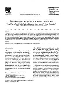
This Section contains two illustrative examples, one mechanical system and one process engineering system. The former is represented by a true (energy conserving) bond graph; the latter is represented by a pseudo bond graph. Further examples appear in a conference paper (Gawthrop et al. (1991a)). 6.1. DC drive with flexibility. The bond graph of a voltage-driven DC motor with armature resistance 1 2 , armature inductance 0.1H, inertia 1 k g m 2, and gain 1 N m A -1 driving an unknown load of mass k through a flexible shaft of stiffness 1 Nm tad -1, is shown in Fig. 1. The 1-junction labeled a corresponds to the motor armature: the armature resistance ra and the armature inductance ia are in series. The gyrator labeled km represents the (energy conserving) transformation from the electrical to the mechanical domain and vice versa. The 1-junction labeled m represents the mechanical part of the motor with common velocity shared by the inertia labeled j m and a measurement device labeled vm. The 0-junction labeled s represents the flexible drive shaft carrying a
I:jm
C:ks
l:m
""x O:s
M:vln
FIo. 1. DC drive with flexibility: bond graph.
I:jl
~
I:I
834
Brief Paper P a r a r n e m r estimates
common torque across the compliance labeled Its. The load inertia is represented by the inertia labeled jl. The corresponding transfer function is (lO(ks z + 1)) G(s) = ((s3 + lOsZ + l l s + 10)ks + s 2 + 10s + 10)"
iiiiiiiiiiii
'
iiiiiiiiiii i iii,
iiiiiiiiiiiii ii
This system is linear in the single parameter k, although the system is quite complex. The corresponding matrix O is
...... ! -
o
.
.
O= .
.
l
.
.
~
.
.
.
.
.
.
.
.
.
.
~
5 6 Time(s~:)
.
.
-10
!
~
~
6
~o
G Product
Stage 3
Stage 2
Stage 1
R:rl2
R:r23
C:c2
1
R.~3
C:c3
f l : f l 2
'N 0:xl
S:ye
l:fl
S
0:x2
R:rl
0:x3
~ l : t 2 1
M:x_l
R:r21
(26)
The time constant r is related to known quantities involving gas and liquid (l) flows and holdups, and can thus be
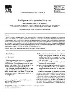
FIG. 3. A three-stage absorber.
1
(25)
(k ~) (((k + st + 1)(3st + 1)k + (st + 1)3 + k3)l) "
Feed
C:cl
10 11 10 1 0 0 -10
This system was simulated with a value of k = 10 kg and a unit step input for 10 sec. Using the software described in Section 5, the estimation algorithm was applied to the system using fl = 0.1, So = 10-4 and C ( s ) = (1 + s) s. The estimation was repeated with three different starting values k o = 0, 5, 20. The corresponding estimates (as a function of time~ appear superimposed in Fig. 2. In each case, the estimate k converges to k = 10. 6.2. A three-stage absorber. The three-stage absorber depicted in Fig. 3 is discussed in detail in a standard chemical engineering textbook (Seborg et al. (1989)). The (pseudo) bond graph appears in Fig. 4. The application of bond graphs to this area is discussed elsewhere (MacKenzie et al. (1991)). The junctions labeled xl, x2, and x3 are common concentration junctions carrying the component concentration of each stage. The junctions labeled 112 and 123 carry the component flows from Stage 1 to Stage 2 and from Stage 2 to Stage 3, respectively; the junctions labeled 132 and t21 carry the flows in the reverse direction. The C components represent the component holdup in each stage. The R components are expressed in terms of the flows transporting the component. Expressed incrementally, the transfer function relating feed changes to product changes is given by
Fro. 2. DC drive with flexibility; estimate of k.
L
(li0 10 1
iiiiiiiiiiiiiiiiiiiiiiiiiiiiiiiiiii
¸¸¸,¸ .
(24)
L
R:r32
FIG. 4. A three-stage absorber: bond graph.
1
Brief Paper System output (-)
835
1.2
0.1
T
': 1.1
0.08 1 0.06
0.9 0.8
0.04
0.7 0.02 0.6 0.5 0.4 -0.02
0.5
1
1.5
2
2.5
3
3.5
4
FIG. 7. Three-stage absorber: estimate of k (varying
C(s)).
3.5
0.5
1
1.5
2
Time (~c)
FIG. 5. Three-stage absorber: simulated data.
regarded as known. The separation factor k is, however, an empirical constant that cannot be easily deduced from first principles; it is regarded as unknown here. The transfer function coefficients contain k raised to the third power. The matrix O is given by: 31r O = 13lr 2 ~l~ 3
' 41r 31r 2 0 0
2.5
3
Time (sec)
'')
31T 0 0 0
0 0 0 -1
.
(27)
the effect of C(s) three simulations where performed as before except that the initial parameter estimate was chosen as ko = 1, and C(s) chosen to be C ( s ) = (1 + s T ) 4 with T = 0.5, 1, 2. The corresponding estimates appear superimposed in Fig. 7. The smallest value of T = 0.5 gives relatively fast, but oscillatory convergence; the largest value of T = 2 gives a relatively slower, but smoother, convergence of the parameter estimate k.
7. Local minima
The system was simulated with k = 0.72, r = 2 and I = 0.5. For additional realism, random numbers (uniformly distributed between - 0 . 0 2 and 0.02) were added to the data, which appear in Fig. 5. Using the software described in Section 5, the estimation algorithm was applied to this set of data. The estimation parameters were: fl = 0.1, So = 10 -4 and C(s) = (1 + s) 4. The simulation was repeated with five different starting values k 0 = 0 , 0.25, 0.5, 0.75, 1. The corresponding estimates appear superimposed in Fig. 6. In the latter four cases, the estimate k converges to k = 0.72; but convergence does not occur in the first case. This is symptomatic of a local minimum at/~ ~- -0.25. The filter polynomial C(s) appearing in equation (2) is chosen by the user; its primary role is to avoid data differentiation. However, it has a secondary role in actually changing the function g(X(s), O) of equation (2) and hence the cost function of equation (11). Different choices of C(s) thus give rise to different parameter estimates 0 although the parameter vector 0 is independent of C(s). To investigate
If the system is Nth order in k, then the cost function is of order 2N. If N = 1 (linear in the parameters) then there can only be one minimum which must therefore be a global minimum. But, if N > 1, multiple minima may exist. As a by-product, the algorithm generates the 2N derivatives of the cost function, and so, as the cost is of order 2N, it can be computed (as a function of/~, equation (11)) at each time t. The cost has been computed for the second example (Section 6.2) at the final time tf = 4 displayed in Fig. 8. The cost function for each of the three values of T is normalized:
7(/~(tf), tf) J(/~(t0, tO - J(/~(t0, t,)
and plotted against/c(t0./c is that (minimizing) value of/c(tf) computed by the algorithm. The costs for the three values of t are quite similar. It can be seen that there are two minima, one (the lowest) at / ~ = / ~ = k = 0 . 7 2 and one at / ~ = / ~ - 0 . 2 5 . The latter minimum is found in the simulation starting with/~ = k = 0 in Section 6.2.
1
0.4
0.8
0.35
0,6
o.31
0.4
o.251 J
(28)
.t(~(tf), t,)
o.21
0.2
o.151
0
Oal -0.2 -0.4 0.5
1.5
2
2.5
3
3.5
Time (sec)
FIG. 6. Three-stage absorber: estimate of k (varying k0).
-I
-O.S
-0.6
-0.4
-{).2
0
0.2
0.4
0.6
O.S
F.slftmv~d k
FIG. 8. Three-stage absorber: cost function (varying
C(s)).
836
Brief Paper
8. Conclusions An algorithm for identifying a single unknown parameter in a partially-known linear system has been described, implemented and verified using two simulated examples. The key ideas developed are as follows. • The use of automatic modelling techniques, based on bond graphs to give a general algorithm capable of expressing particular systems properties. • The use of polynomial in the parameter identification techniques. Immediate objectives for future work are to: • investigate further the problem of local minima, • understand the effect of C(s) on algorithm performance, • extend the method to multiple unknown parameters, • extend the method to nonlinear systems, • apply the method to real data arising from: (i) process engineering systems, (ii) robotic systems, • develop corresponding adaptive control techniques for partially-known systems. A longer term objective is to capture functional as opposed to parametric uncertainty in the context of partially-known systems. Acknowledgements--The ideas expressed in this paper arise from interdisciplinary research within the Control Systems Group at Glasgow University and all of the group have contributed ideas directly and indirectly. The ideas about partially-known systems arose from a project sponsored by SERC in collaboration with J. W. Ponton at Edinburgh University Chemical Engineering Department. The modelling tools were developed in conjunction with the Engineering Design Research Centre. The flexible drive example, and the idea of metamodelling, arose from an ACME sponsored project in conjunction with Lamberton Robotics.
References Anderson, M. (1989). Omola--an object-orientated modelling language. Report TFRT 7417, Lund Institute of Technology. CIocksin, W. F. and C. S. Mellish (1984). Programming in Prolog (2nd edition). Springer-Verlag, Berlin. Dasgupta S., B. D. O. Anderson and R. J. Kaye (1986). Output error identification methods for partially known systems. Int. J. Control, 43, 177-91. Canudas de Wit, C. A. (1988). Adaptive Control for Partially Known Systems. Elsevier, Amsterdam. Gawthrop, P. J. and M. T. Nihtila (1985). Identification of time-delays using a polynomial identification method. Systems and Control Letters, 5, 267-271. Gawthrop, P. J. and M. T. Nihtila (1991). Identification of distributed parameter systems using polynomial identification techniques. 9th IFAC/IFORS Symposium on Identification and System Parameter Estimation. Budapest, Hungary, pp. 975-980. Gawthrop, P. J. and L. Smith (1990). An environment for specification, design, operation, maintenance, and revision
of manufacturing control systems. Proc. of UKIT90 pp. 104-110. Gawthrop, P. J., M. T. Hihtila and A. Besharati-Rad (1989). Recursive parameter estimation of continuous-time systems with unknown time delay. C-TAT, 15. Gawthrop, P. J., R. W. Jones and S. A. MacKenzie (1991). Identification of partially-known systems. 9th 1FAC/IFORS symposium on identification and system parameter estimation. Budapest, Hungary, pp. 1347-1352. Gawthrop, P. J., N. A. Marrison and L. Smith (1991). M'IT: A bond graph toolbox. Proc. of the 5th 1FAC/IMACS Symposium on Computer-aided Design of Control Systems: CADCS91. Gawthrop, P. J. (1987). Continuous-time Self-tuning Control. Vol 1: Design. Research Studies Press, Engineering control series, Letchworth, U.K. Gawthrop, P. J. (1990). Continuous-time Self-tuning Control. Vol 2: Implementation. Research Studies Press, Engineering control series, Taunton, U.K. Karnopp, D. C. and R. C. Rosenberg (1975). System Dynamics: A Unified Approach. John Wiley, New York. Karnopp, D. C., D. L. Margolis and R. C. Rosenberg (1990). System Dynamics: A Unified Approach. John Wiley, New York. MacKenzie, S., P. J. Gawthrop, R. W. Jones and J. W. Ponton (1991). Systematic modelling of chemical processes. IFAC symposium on Advanced Control of Chemical Processes, ADCHEM91. Toulouse, France. Mattsson, S. E. and M. Anderson (1990). A kernel for system representation. Preprints of llth IFAC world congress, Vol. 10, pp. 91-96. Tallinn, Estonia. Moler, C., J. Little and S. Bangert (1987). MATLAB User's Guide. Mathworks, South Natizk, MA. Nagy, P. A. J. and L. Ljung (1991). Computer-aided model structure selection. Preprints of 9th IFAC/IFORS Symposium on Identification and System Parameter Estimation, Budapest, Hungary, pp. 918-923. Nagy, P. A. J. and L. Ljung. System identification using bond graphs. Proc. of the First European Control Conference, pp. 2564-2569. Grenoble, Hermes. Nagy, P. A. J. (1991). Bond tool m: An interactive interface to the system identification toolbox. Report LiTH-ISY-I1264, Department of Electrical Engineering, Linkoping University,. Nihtila, M. T. (1983). Optimal finite dimensional recursive identification in a polynomial output mapping class. Systems and Control Letters, 3, 341-348. Rayna, G. (1987). Reduce: Software for Algebraic Computation. Springer-Verlag, Berlin. Rosenberg, R. C. and D. C. Karnopp (1983). Introduction to Physical System Dynamics. McGraw-Hill, New York. Seborg, D. E., T. F. Edgar and D. A. Mellichamp (1989). Process Dynamics and Control. John Wiley, New York. Thoma, J. U. (1990). Simulation by Bond Graphs. Springer-Verlag, Berlin. Unbehauen, H. and G. P. Rao (1987). Identification of Continuous Systems. North Holland, Amsterdam. Welistead P. E. (1979). Introduction to Physical System Modelling. Academic Press New York. Young, P. C. (1981). Parameter estimation for continuoustime models---a survey. Automatica, 17, 23-39.