FLUENT 6.3 Tutorial Guide

FLUENT 6.3

September 2006

Tutorial Guide

c 2006 by Fluent Inc. Copyright All Rights Reserved. No part of this document may be reproduced or otherwise used in any form without express written permission from Fluent Inc.

Airpak, FIDAP, FLUENT, FLUENT for CATIA V5, FloWizard, GAMBIT, Icemax, Icepak, Icepro, Icewave, Icechip, MixSim, and POLYFLOW are registered trademarks of Fluent Inc. All other products or name brands are trademarks of their respective holders. CHEMKIN is a registered trademark of Reaction Design Inc. Portions of this program include material copyrighted by PathScale Corporation 2003-2004.

Fluent Inc. Centerra Resource Park 10 Cavendish Court Lebanon, NH 03766

Volume 1 1 2 3 4 5 6 7 8 9 10 11

Introduction to Using FLUENT: Fluid Flow and Heat Transfer in a Mixing Elbow Modeling Periodic Flow and Heat Transfer Modeling External Compressible Flow Modeling Unsteady Compressible Flow Modeling Radiation and Natural Convection Using a Non-Conformal Mesh Using a Single Rotating Reference Frame Using Multiple Rotating Reference Frames Using the Mixing Plane Model Using Sliding Meshes Using Dynamic Meshes

Volume 2 12 13 14 15 16 17 18 19 20 21 22 23 24

Modeling Species Transport and Gaseous Combustion Using the Non-Premixed Combustion Model Modeling Surface Chemistry Modeling Evaporating Liquid Spray Using the VOF Model Modeling Cavitation Using the Mixture and Eulerian Multiphase Models Using the Eulerian Multiphase Model for Granular Flow Modeling Solidification Using the Eulerian Granular Multiphase Model with Heat Transfer Postprocessing Turbo Postprocessing Parallel Processing

Contents

1 Introduction to Using FLUENT: Fluid Flow and Heat Transfer in a Mixing Elbow

1-1

Introduction . . . . . . . . . . . . . . . . . . . . . . . . . . . . . . . . . . . . .

1-1

Prerequisites

. . . . . . . . . . . . . . . . . . . . . . . . . . . . . . . . . . . .

1-1

Problem Description . . . . . . . . . . . . . . . . . . . . . . . . . . . . . . . .

1-2

Setup and Solution . . . . . . . . . . . . . . . . . . . . . . . . . . . . . . . . .

1-3

Preparation . . . . . . . . . . . . . . . . . . . . . . . . . . . . . . . . . .

1-3

Step 1: Grid . . . . . . . . . . . . . . . . . . . . . . . . . . . . . . . . . .

1-4

Step 2: Models . . . . . . . . . . . . . . . . . . . . . . . . . . . . . . . .

1-9

Step 3: Materials . . . . . . . . . . . . . . . . . . . . . . . . . . . . . . . 1-11 Step 4: Boundary Conditions . . . . . . . . . . . . . . . . . . . . . . . . 1-13 Step 5: Solution . . . . . . . . . . . . . . . . . . . . . . . . . . . . . . . . 1-19 Step 6: Displaying the Preliminary Solution . . . . . . . . . . . . . . . . 1-28 Step 7: Enabling Second-Order Discretization . . . . . . . . . . . . . . . 1-39 Step 8: Adapting the Grid . . . . . . . . . . . . . . . . . . . . . . . . . . 1-46 Summary . . . . . . . . . . . . . . . . . . . . . . . . . . . . . . . . . . . . . . 1-58 2 Modeling Periodic Flow and Heat Transfer

2-1

Introduction . . . . . . . . . . . . . . . . . . . . . . . . . . . . . . . . . . . . .

2-1

Prerequisites

. . . . . . . . . . . . . . . . . . . . . . . . . . . . . . . . . . . .

2-1


2-2


2-3

Preparation . . . . . . . . . . . . . . . . . . . . . . . . . . . . . . . . . .

2-3

Step 1: Grid . . . . . . . . . . . . . . . . . . . . . . . . . . . . . . . . . .

2-3

Step 2: Models . . . . . . . . . . . . . . . . . . . . . . . . . . . . . . . .

2-6

c Fluent Inc. September 21, 2006

i

CONTENTS

Step 3: Materials . . . . . . . . . . . . . . . . . . . . . . . . . . . . . . .

2-8

Step 4: Boundary Conditions . . . . . . . . . . . . . . . . . . . . . . . . 2-10 Step 5: Solution . . . . . . . . . . . . . . . . . . . . . . . . . . . . . . . . 2-13 Step 6: Postprocessing . . . . . . . . . . . . . . . . . . . . . . . . . . . . 2-16 Summary . . . . . . . . . . . . . . . . . . . . . . . . . . . . . . . . . . . . . . 2-25 Further Improvements . . . . . . . . . . . . . . . . . . . . . . . . . . . . . . . 2-25 3 Modeling External Compressible Flow

3-1

Introduction . . . . . . . . . . . . . . . . . . . . . . . . . . . . . . . . . . . . .

3-1

Prerequisites

. . . . . . . . . . . . . . . . . . . . . . . . . . . . . . . . . . . .

3-1


3-2


3-2

Preparation . . . . . . . . . . . . . . . . . . . . . . . . . . . . . . . . . .

3-2

Step 1: Grid . . . . . . . . . . . . . . . . . . . . . . . . . . . . . . . . . .

3-3

Step 2: Models . . . . . . . . . . . . . . . . . . . . . . . . . . . . . . . .

3-5

Step 3: Materials . . . . . . . . . . . . . . . . . . . . . . . . . . . . . . .

3-7

Step 4: Operating Conditions . . . . . . . . . . . . . . . . . . . . . . . .

3-8

Step 5: Boundary Conditions . . . . . . . . . . . . . . . . . . . . . . . .

3-9

Step 6: Solution . . . . . . . . . . . . . . . . . . . . . . . . . . . . . . . . 3-11 Step 7: Postprocessing . . . . . . . . . . . . . . . . . . . . . . . . . . . . 3-25 Summary . . . . . . . . . . . . . . . . . . . . . . . . . . . . . . . . . . . . . . 3-31 Further Improvements . . . . . . . . . . . . . . . . . . . . . . . . . . . . . . . 3-31 4 Modeling Unsteady Compressible Flow

ii

4-1

Introduction . . . . . . . . . . . . . . . . . . . . . . . . . . . . . . . . . . . . .

4-1

Prerequisites

. . . . . . . . . . . . . . . . . . . . . . . . . . . . . . . . . . . .

4-1


4-1


4-2

Preparation . . . . . . . . . . . . . . . . . . . . . . . . . . . . . . . . . .

4-2

Step 1: Grid . . . . . . . . . . . . . . . . . . . . . . . . . . . . . . . . . .

4-3


CONTENTS

Step 2: Units . . . . . . . . . . . . . . . . . . . . . . . . . . . . . . . . .

4-5

Step 3: Models . . . . . . . . . . . . . . . . . . . . . . . . . . . . . . . .

4-6

Step 4: Materials . . . . . . . . . . . . . . . . . . . . . . . . . . . . . . .

4-8

Step 5: Operating Conditions . . . . . . . . . . . . . . . . . . . . . . . .

4-9

Step 6: Boundary Conditions . . . . . . . . . . . . . . . . . . . . . . . . 4-10 Step 7: Solution: Steady Flow . . . . . . . . . . . . . . . . . . . . . . . . 4-12 Step 8: Enable Time Dependence and Set Unsteady Conditions . . . . . 4-24 Step 9: Solution: Unsteady Flow . . . . . . . . . . . . . . . . . . . . . . 4-27 Step 10: Saving and Postprocessing Time-Dependent Data Sets . . . . . 4-30 Summary . . . . . . . . . . . . . . . . . . . . . . . . . . . . . . . . . . . . . . 4-43 Further Improvements . . . . . . . . . . . . . . . . . . . . . . . . . . . . . . . 4-43 5 Modeling Radiation and Natural Convection

5-1

Introduction . . . . . . . . . . . . . . . . . . . . . . . . . . . . . . . . . . . . .

5-1

Prerequisites

. . . . . . . . . . . . . . . . . . . . . . . . . . . . . . . . . . . .

5-1


5-1


5-2

Preparation . . . . . . . . . . . . . . . . . . . . . . . . . . . . . . . . . .

5-2

Step 1: Grid . . . . . . . . . . . . . . . . . . . . . . . . . . . . . . . . . .

5-3

Step 2: Models . . . . . . . . . . . . . . . . . . . . . . . . . . . . . . . .

5-6

Step 3: Materials . . . . . . . . . . . . . . . . . . . . . . . . . . . . . . .

5-8


5-9

Step 5: Solution for the Rosseland Model . . . . . . . . . . . . . . . . . . 5-12 Step 6: Postprocessing for the Rosseland Model . . . . . . . . . . . . . . 5-15 Step 7: P-1 Model Setup, Solution, and Postprocessing . . . . . . . . . . 5-24 Step 8: DTRM Setup, Solution, and Postprocessing . . . . . . . . . . . . 5-28 Step 9: DO Model Setup, Solution, and Postprocessing . . . . . . . . . . 5-31 Step 10: Comparison of y-Velocity Plots . . . . . . . . . . . . . . . . . . 5-34 Step 11: Comparison of Radiation Models for an Optically Thick Medium . . . . . . . . . . . . . . . . . . . . . . . . . . . . 5-36


iii

CONTENTS

Step 12: S2S Setup, Solution, and Postprocessing for a Non-Participating Medium . . . . . . . . . . . . . . . . . . . . . 5-38 Step 13: Comparison of Radiation Models for a Non-Participating Medium . . . . . . . . . . . . . . . . . . . . . 5-43 Step 14: S2S Definition, Solution and Postprocessing with Partial Enclosure . . . . . . . . . . . . . . . . . . . . . . . . . . . 5-45 Step 15: Comparison of S2S Models with and without Partial Enclosure . 5-49 Summary . . . . . . . . . . . . . . . . . . . . . . . . . . . . . . . . . . . . . . 5-50 Further Improvements . . . . . . . . . . . . . . . . . . . . . . . . . . . . . . . 5-50 6 Using a Non-Conformal Mesh

6-1

Introduction . . . . . . . . . . . . . . . . . . . . . . . . . . . . . . . . . . . . .

6-1

Prerequisites

. . . . . . . . . . . . . . . . . . . . . . . . . . . . . . . . . . . .

6-1


6-2


6-3

Preparation . . . . . . . . . . . . . . . . . . . . . . . . . . . . . . . . . .

6-3

Step 1: Merging the Mesh Files . . . . . . . . . . . . . . . . . . . . . . .

6-3

Step 2: Grid . . . . . . . . . . . . . . . . . . . . . . . . . . . . . . . . . .

6-4

Step 3: Models . . . . . . . . . . . . . . . . . . . . . . . . . . . . . . . .

6-7

Step 4: Materials . . . . . . . . . . . . . . . . . . . . . . . . . . . . . . .

6-9

Step 5: Operating Conditions . . . . . . . . . . . . . . . . . . . . . . . . 6-10 Step 6: Boundary Conditions . . . . . . . . . . . . . . . . . . . . . . . . 6-10 Step 7: Grid Interfaces . . . . . . . . . . . . . . . . . . . . . . . . . . . . 6-20 Step 8: Solution . . . . . . . . . . . . . . . . . . . . . . . . . . . . . . . . 6-22 Step 9: Postprocessing . . . . . . . . . . . . . . . . . . . . . . . . . . . . 6-25 Summary . . . . . . . . . . . . . . . . . . . . . . . . . . . . . . . . . . . . . . 6-33 Further Improvements . . . . . . . . . . . . . . . . . . . . . . . . . . . . . . . 6-33

iv


CONTENTS

7 Modeling Flow Through Porous Media

7-1

Introduction . . . . . . . . . . . . . . . . . . . . . . . . . . . . . . . . . . . . .

7-1

Prerequisites

. . . . . . . . . . . . . . . . . . . . . . . . . . . . . . . . . . . .

7-1


7-2


7-2

Preparation . . . . . . . . . . . . . . . . . . . . . . . . . . . . . . . . . .

7-2

Step 1: Grid . . . . . . . . . . . . . . . . . . . . . . . . . . . . . . . . . .

7-3

Step 2: Models . . . . . . . . . . . . . . . . . . . . . . . . . . . . . . . .

7-5

Step 3: Materials . . . . . . . . . . . . . . . . . . . . . . . . . . . . . . .

7-7


7-9

Step 5: Solution . . . . . . . . . . . . . . . . . . . . . . . . . . . . . . . . 7-14 Step 6: Postprocessing . . . . . . . . . . . . . . . . . . . . . . . . . . . . 7-18 Summary . . . . . . . . . . . . . . . . . . . . . . . . . . . . . . . . . . . . . . 7-32 Further Improvements . . . . . . . . . . . . . . . . . . . . . . . . . . . . . . . 7-32 8 Using a Single Rotating Reference Frame

8-1

Introduction . . . . . . . . . . . . . . . . . . . . . . . . . . . . . . . . . . . . .

8-1

Prerequisites

. . . . . . . . . . . . . . . . . . . . . . . . . . . . . . . . . . . .

8-1


8-1


8-3

Preparation . . . . . . . . . . . . . . . . . . . . . . . . . . . . . . . . . .

8-3

Step 1: Grid . . . . . . . . . . . . . . . . . . . . . . . . . . . . . . . . . .

8-3

Step 2: Units . . . . . . . . . . . . . . . . . . . . . . . . . . . . . . . . .

8-5

Step 3: Models . . . . . . . . . . . . . . . . . . . . . . . . . . . . . . . .

8-6

Step 4: Materials . . . . . . . . . . . . . . . . . . . . . . . . . . . . . . .

8-8


8-9

Step 6: Solution Using the Standard k- Model

. . . . . . . . . . . . . . 8-13

Step 7: Postprocessing for the Standard k- Solution . . . . . . . . . . . 8-19 Step 8: Solution Using the RNG k- Model . . . . . . . . . . . . . . . . . 8-25


v

CONTENTS

Step 9: Postprocessing for the RNG k- Solution . . . . . . . . . . . . . . 8-26 Summary . . . . . . . . . . . . . . . . . . . . . . . . . . . . . . . . . . . . . . 8-29 Further Improvements . . . . . . . . . . . . . . . . . . . . . . . . . . . . . . . 8-29 References . . . . . . . . . . . . . . . . . . . . . . . . . . . . . . . . . . . . . . 8-30 9 Using Multiple Rotating Reference Frames

9-1

Introduction . . . . . . . . . . . . . . . . . . . . . . . . . . . . . . . . . . . . .

9-1

Prerequisites

. . . . . . . . . . . . . . . . . . . . . . . . . . . . . . . . . . . .

9-1


9-2


9-3

Preparation . . . . . . . . . . . . . . . . . . . . . . . . . . . . . . . . . .

9-3

Step 1: Grid . . . . . . . . . . . . . . . . . . . . . . . . . . . . . . . . . .

9-3

Step 2: Models . . . . . . . . . . . . . . . . . . . . . . . . . . . . . . . .

9-6

Step 3: Materials . . . . . . . . . . . . . . . . . . . . . . . . . . . . . . .

9-7


9-8

Step 5: Solution . . . . . . . . . . . . . . . . . . . . . . . . . . . . . . . . 9-13 Step 6: Postprocessing . . . . . . . . . . . . . . . . . . . . . . . . . . . . 9-16 Summary . . . . . . . . . . . . . . . . . . . . . . . . . . . . . . . . . . . . . . 9-19 Further Improvements . . . . . . . . . . . . . . . . . . . . . . . . . . . . . . . 9-20 10 Using the Mixing Plane Model

10-1

Introduction . . . . . . . . . . . . . . . . . . . . . . . . . . . . . . . . . . . . . 10-1 Prerequisites

. . . . . . . . . . . . . . . . . . . . . . . . . . . . . . . . . . . . 10-1

Problem Description . . . . . . . . . . . . . . . . . . . . . . . . . . . . . . . . 10-1 Setup and Solution . . . . . . . . . . . . . . . . . . . . . . . . . . . . . . . . . 10-2 Preparation . . . . . . . . . . . . . . . . . . . . . . . . . . . . . . . . . . 10-2 Step 1: Grid . . . . . . . . . . . . . . . . . . . . . . . . . . . . . . . . . . 10-3 Step 2: Units . . . . . . . . . . . . . . . . . . . . . . . . . . . . . . . . . 10-4 Step 3: Models . . . . . . . . . . . . . . . . . . . . . . . . . . . . . . . . 10-5 Step 4: Mixing Plane . . . . . . . . . . . . . . . . . . . . . . . . . . . . . 10-7

vi


CONTENTS

Step 5: Materials . . . . . . . . . . . . . . . . . . . . . . . . . . . . . . . 10-9 Step 6: Boundary Conditions . . . . . . . . . . . . . . . . . . . . . . . . 10-10 Step 7: Solution . . . . . . . . . . . . . . . . . . . . . . . . . . . . . . . . 10-21 Step 8: Postprocessing . . . . . . . . . . . . . . . . . . . . . . . . . . . . 10-27 Summary . . . . . . . . . . . . . . . . . . . . . . . . . . . . . . . . . . . . . . 10-32 Further Improvements . . . . . . . . . . . . . . . . . . . . . . . . . . . . . . . 10-32 11 Using Sliding Meshes

11-1


. . . . . . . . . . . . . . . . . . . . . . . . . . . . . . . . . . . . 11-1

Problem Description . . . . . . . . . . . . . . . . . . . . . . . . . . . . . . . . 11-1 Setup and Solution . . . . . . . . . . . . . . . . . . . . . . . . . . . . . . . . . 11-3 Preparation . . . . . . . . . . . . . . . . . . . . . . . . . . . . . . . . . . 11-3 Step 1: Grid . . . . . . . . . . . . . . . . . . . . . . . . . . . . . . . . . . 11-3 Step 2: Models . . . . . . . . . . . . . . . . . . . . . . . . . . . . . . . . 11-7 Step 3: Materials . . . . . . . . . . . . . . . . . . . . . . . . . . . . . . . 11-9 Step 4: Operating Conditions . . . . . . . . . . . . . . . . . . . . . . . . 11-10 Step 5: Boundary Conditions . . . . . . . . . . . . . . . . . . . . . . . . 11-11 Step 6: Grid Interfaces . . . . . . . . . . . . . . . . . . . . . . . . . . . . 11-16 Step 7: Solution . . . . . . . . . . . . . . . . . . . . . . . . . . . . . . . . 11-17 Step 8: Postprocessing . . . . . . . . . . . . . . . . . . . . . . . . . . . . 11-31 Summary . . . . . . . . . . . . . . . . . . . . . . . . . . . . . . . . . . . . . . 11-37 Further Improvements . . . . . . . . . . . . . . . . . . . . . . . . . . . . . . . 11-37 12 Using Dynamic Meshes

12-1


. . . . . . . . . . . . . . . . . . . . . . . . . . . . . . . . . . . . 12-1

Problem Description . . . . . . . . . . . . . . . . . . . . . . . . . . . . . . . . 12-2 Setup and Solution . . . . . . . . . . . . . . . . . . . . . . . . . . . . . . . . . 12-2 Preparation . . . . . . . . . . . . . . . . . . . . . . . . . . . . . . . . . . 12-2


vii

CONTENTS

Step 1: Grid . . . . . . . . . . . . . . . . . . . . . . . . . . . . . . . . . . 12-3 Step 2: Models . . . . . . . . . . . . . . . . . . . . . . . . . . . . . . . . 12-4 Step 3: Materials . . . . . . . . . . . . . . . . . . . . . . . . . . . . . . . 12-6 Step 4: Boundary Conditions . . . . . . . . . . . . . . . . . . . . . . . . 12-7 Step 5: Solution: Steady Flow . . . . . . . . . . . . . . . . . . . . . . . . 12-10 Step 6: Unsteady Solution Setup . . . . . . . . . . . . . . . . . . . . . . 12-12 Step 7: Mesh Motion . . . . . . . . . . . . . . . . . . . . . . . . . . . . . 12-13 Step 8: Unsteady Solution . . . . . . . . . . . . . . . . . . . . . . . . . . 12-19 Step 9: Postprocessing . . . . . . . . . . . . . . . . . . . . . . . . . . . . 12-26 Summary . . . . . . . . . . . . . . . . . . . . . . . . . . . . . . . . . . . . . . 12-29 Further Improvements . . . . . . . . . . . . . . . . . . . . . . . . . . . . . . . 12-29 13 Modeling Species Transport and Gaseous Combustion

13-1


. . . . . . . . . . . . . . . . . . . . . . . . . . . . . . . . . . . . 13-1

Problem Description . . . . . . . . . . . . . . . . . . . . . . . . . . . . . . . . 13-1 Background . . . . . . . . . . . . . . . . . . . . . . . . . . . . . . . . . . . . . 13-2 Setup and Solution . . . . . . . . . . . . . . . . . . . . . . . . . . . . . . . . . 13-3 Preparation . . . . . . . . . . . . . . . . . . . . . . . . . . . . . . . . . . 13-3 Step 1: Grid . . . . . . . . . . . . . . . . . . . . . . . . . . . . . . . . . . 13-3 Step 2: Models . . . . . . . . . . . . . . . . . . . . . . . . . . . . . . . . 13-5 Step 3: Materials . . . . . . . . . . . . . . . . . . . . . . . . . . . . . . . 13-9 Step 4: Boundary Conditions . . . . . . . . . . . . . . . . . . . . . . . . 13-13 Step 5: Initial Solution with Constant Heat Capacity . . . . . . . . . . . 13-21 Step 6: Solution with Varying Heat Capacity . . . . . . . . . . . . . . . . 13-26 Step 7: Postprocessing . . . . . . . . . . . . . . . . . . . . . . . . . . . . 13-29 Step 8: NOx Prediction . . . . . . . . . . . . . . . . . . . . . . . . . . . . 13-37 Summary . . . . . . . . . . . . . . . . . . . . . . . . . . . . . . . . . . . . . . 13-47 Further Improvements . . . . . . . . . . . . . . . . . . . . . . . . . . . . . . . 13-47

viii


CONTENTS

14 Using the Non-Premixed Combustion Model

14-1


. . . . . . . . . . . . . . . . . . . . . . . . . . . . . . . . . . . . 14-1

Problem Description . . . . . . . . . . . . . . . . . . . . . . . . . . . . . . . . 14-2 Setup and Solution . . . . . . . . . . . . . . . . . . . . . . . . . . . . . . . . . 14-3 Preparation . . . . . . . . . . . . . . . . . . . . . . . . . . . . . . . . . . . . . 14-3 Step 1: Grid . . . . . . . . . . . . . . . . . . . . . . . . . . . . . . . . . . 14-4 Step 2: Models . . . . . . . . . . . . . . . . . . . . . . . . . . . . . . . . 14-8 Step 3: Non Adiabatic PDF Table . . . . . . . . . . . . . . . . . . . . . . 14-12 Step 4: Materials . . . . . . . . . . . . . . . . . . . . . . . . . . . . . . . 14-16 Step 5: Operating Conditions . . . . . . . . . . . . . . . . . . . . . . . . 14-17 Step 6: Boundary Conditions . . . . . . . . . . . . . . . . . . . . . . . . 14-18 Step 7: Solution . . . . . . . . . . . . . . . . . . . . . . . . . . . . . . . . 14-23 Step 8: Postprocessing . . . . . . . . . . . . . . . . . . . . . . . . . . . . 14-26 Step 9: Energy Balances Reporting . . . . . . . . . . . . . . . . . . . . . 14-29 Summary . . . . . . . . . . . . . . . . . . . . . . . . . . . . . . . . . . . . . . 14-30 References . . . . . . . . . . . . . . . . . . . . . . . . . . . . . . . . . . . . . . 14-31 Further Improvements . . . . . . . . . . . . . . . . . . . . . . . . . . . . . . . 14-31 15 Modeling Surface Chemistry

15-1


. . . . . . . . . . . . . . . . . . . . . . . . . . . . . . . . . . . . 15-1

Problem Description . . . . . . . . . . . . . . . . . . . . . . . . . . . . . . . . 15-2 Setup and Solution . . . . . . . . . . . . . . . . . . . . . . . . . . . . . . . . . 15-3 Preparation . . . . . . . . . . . . . . . . . . . . . . . . . . . . . . . . . . 15-3 Step 1: Grid . . . . . . . . . . . . . . . . . . . . . . . . . . . . . . . . . . 15-3 Step 2: Models . . . . . . . . . . . . . . . . . . . . . . . . . . . . . . . . 15-6 Step 3: Materials . . . . . . . . . . . . . . . . . . . . . . . . . . . . . . . 15-9 Step 4: Operating Conditions . . . . . . . . . . . . . . . . . . . . . . . . 15-16


ix

CONTENTS

Step 5: Boundary Conditions . . . . . . . . . . . . . . . . . . . . . . . . 15-17 Step 6: Solution . . . . . . . . . . . . . . . . . . . . . . . . . . . . . . . . 15-22 Step 7: Postprocessing . . . . . . . . . . . . . . . . . . . . . . . . . . . . 15-26 Summary . . . . . . . . . . . . . . . . . . . . . . . . . . . . . . . . . . . . . . 15-32 Further Improvements . . . . . . . . . . . . . . . . . . . . . . . . . . . . . . . 15-32 16 Modeling Evaporating Liquid Spray

16-1


. . . . . . . . . . . . . . . . . . . . . . . . . . . . . . . . . . . . 16-1

Problem Description . . . . . . . . . . . . . . . . . . . . . . . . . . . . . . . . 16-1 Setup and Solution . . . . . . . . . . . . . . . . . . . . . . . . . . . . . . . . . 16-2 Preparation . . . . . . . . . . . . . . . . . . . . . . . . . . . . . . . . . . 16-2 Step 1: Grid . . . . . . . . . . . . . . . . . . . . . . . . . . . . . . . . . . 16-3 Step 2: Models . . . . . . . . . . . . . . . . . . . . . . . . . . . . . . . . 16-7 Step 3: Boundary Conditions . . . . . . . . . . . . . . . . . . . . . . . . 16-10 Step 4: Initial Solution Without Droplets . . . . . . . . . . . . . . . . . . 16-16 Step 5: Create a Spray Injection . . . . . . . . . . . . . . . . . . . . . . . 16-25 Step 6: Solution . . . . . . . . . . . . . . . . . . . . . . . . . . . . . . . . 16-32 Step 7: Postprocessing . . . . . . . . . . . . . . . . . . . . . . . . . . . . 16-34 Summary . . . . . . . . . . . . . . . . . . . . . . . . . . . . . . . . . . . . . . 16-38 Further Improvements . . . . . . . . . . . . . . . . . . . . . . . . . . . . . . . 16-38 17 Using the VOF Model

17-1


. . . . . . . . . . . . . . . . . . . . . . . . . . . . . . . . . . . . 17-1

Problem Description . . . . . . . . . . . . . . . . . . . . . . . . . . . . . . . . 17-1 Setup and Solution . . . . . . . . . . . . . . . . . . . . . . . . . . . . . . . . . 17-3 Preparation . . . . . . . . . . . . . . . . . . . . . . . . . . . . . . . . . . 17-3 Step 1: Grid . . . . . . . . . . . . . . . . . . . . . . . . . . . . . . . . . . 17-4 Step 2: Models . . . . . . . . . . . . . . . . . . . . . . . . . . . . . . . . 17-9

x


CONTENTS

Step 3: Materials . . . . . . . . . . . . . . . . . . . . . . . . . . . . . . . 17-11 Step 4: Phases

. . . . . . . . . . . . . . . . . . . . . . . . . . . . . . . . 17-13

Step 5: Operating Conditions . . . . . . . . . . . . . . . . . . . . . . . . 17-15 Step 6: User-Defined Function (UDF) . . . . . . . . . . . . . . . . . . . . 17-15 Step 7: Boundary Conditions . . . . . . . . . . . . . . . . . . . . . . . . 17-16 Step 8: Solution . . . . . . . . . . . . . . . . . . . . . . . . . . . . . . . . 17-21 Step 9: Postprocessing . . . . . . . . . . . . . . . . . . . . . . . . . . . . 17-27 Summary . . . . . . . . . . . . . . . . . . . . . . . . . . . . . . . . . . . . . . 17-30 Further Improvements . . . . . . . . . . . . . . . . . . . . . . . . . . . . . . . 17-30 18 Modeling Cavitation

18-1


. . . . . . . . . . . . . . . . . . . . . . . . . . . . . . . . . . . . 18-1

Problem Description . . . . . . . . . . . . . . . . . . . . . . . . . . . . . . . . 18-1 Setup and Solution . . . . . . . . . . . . . . . . . . . . . . . . . . . . . . . . . 18-2 Preparation . . . . . . . . . . . . . . . . . . . . . . . . . . . . . . . . . . 18-2 Step 1: Grid . . . . . . . . . . . . . . . . . . . . . . . . . . . . . . . . . . 18-3 Step 2: Models . . . . . . . . . . . . . . . . . . . . . . . . . . . . . . . . 18-5 Step 3: Materials . . . . . . . . . . . . . . . . . . . . . . . . . . . . . . . 18-8 Step 4: Phases

. . . . . . . . . . . . . . . . . . . . . . . . . . . . . . . . 18-11

Step 5: Operating Conditions . . . . . . . . . . . . . . . . . . . . . . . . 18-13 Step 6: Boundary Conditions . . . . . . . . . . . . . . . . . . . . . . . . 18-14 Step 7: Solution . . . . . . . . . . . . . . . . . . . . . . . . . . . . . . . . 18-18 Step 8: Postprocessing . . . . . . . . . . . . . . . . . . . . . . . . . . . . 18-22 Summary . . . . . . . . . . . . . . . . . . . . . . . . . . . . . . . . . . . . . . 18-26 Further Improvements . . . . . . . . . . . . . . . . . . . . . . . . . . . . . . . 18-26


xi

CONTENTS

19 Using the Mixture and Eulerian Multiphase Models

19-1


. . . . . . . . . . . . . . . . . . . . . . . . . . . . . . . . . . . . 19-1


. . . . . . . . . . . . . . . . . . . . . . . . . . . . . . . . 19-9

Step 5: Boundary Conditions . . . . . . . . . . . . . . . . . . . . . . . . 19-12 Step 6: Solution Using the Mixture Model . . . . . . . . . . . . . . . . . 19-16 Step 7: Postprocessing for the Mixture Solution . . . . . . . . . . . . . . 19-20 Step 8: Setup and Solution for the Eulerian Model . . . . . . . . . . . . . 19-23 Step 9: Postprocessing for the Eulerian Model . . . . . . . . . . . . . . . 19-26 Summary . . . . . . . . . . . . . . . . . . . . . . . . . . . . . . . . . . . . . . 19-28 Further Improvements . . . . . . . . . . . . . . . . . . . . . . . . . . . . . . . 19-28 20 Using the Eulerian Multiphase Model for Granular Flow

20-1


. . . . . . . . . . . . . . . . . . . . . . . . . . . . . . . . . . . . 20-1


. . . . . . . . . . . . . . . . . . . . . . . . . . . . . . . . 20-12

Step 5: User-Defined Function (UDF) . . . . . . . . . . . . . . . . . . . . 20-14

xii


CONTENTS

Step 6: Boundary Conditions . . . . . . . . . . . . . . . . . . . . . . . . 20-16 Step 7: Solution . . . . . . . . . . . . . . . . . . . . . . . . . . . . . . . . 20-18 Step 8: Postprocessing . . . . . . . . . . . . . . . . . . . . . . . . . . . . 20-28 Summary . . . . . . . . . . . . . . . . . . . . . . . . . . . . . . . . . . . . . . 20-30 Further Improvements . . . . . . . . . . . . . . . . . . . . . . . . . . . . . . . 20-30 21 Modeling Solidification

21-1


. . . . . . . . . . . . . . . . . . . . . . . . . . . . . . . . . . . . 21-1

Problem Description . . . . . . . . . . . . . . . . . . . . . . . . . . . . . . . . 21-1 Setup and Solution . . . . . . . . . . . . . . . . . . . . . . . . . . . . . . . . . 21-2 Preparation . . . . . . . . . . . . . . . . . . . . . . . . . . . . . . . . . . 21-2 Step 1: Grid . . . . . . . . . . . . . . . . . . . . . . . . . . . . . . . . . . 21-3 Step 2: Models . . . . . . . . . . . . . . . . . . . . . . . . . . . . . . . . 21-4 Step 3: Materials . . . . . . . . . . . . . . . . . . . . . . . . . . . . . . . 21-7 Step 4: Boundary Conditions . . . . . . . . . . . . . . . . . . . . . . . . 21-9 Step 5: Solution: Steady Conduction . . . . . . . . . . . . . . . . . . . . 21-17 Step 6: Solution: Unsteady Flow and Heat Transfer . . . . . . . . . . . . 21-25 Summary . . . . . . . . . . . . . . . . . . . . . . . . . . . . . . . . . . . . . . 21-31 Further Improvements . . . . . . . . . . . . . . . . . . . . . . . . . . . . . . . 21-31 22 Using the Eulerian Granular Multiphase Model with Heat Transfer 22-1 Introduction . . . . . . . . . . . . . . . . . . . . . . . . . . . . . . . . . . . . . 22-1 Prerequisites

. . . . . . . . . . . . . . . . . . . . . . . . . . . . . . . . . . . . 22-1

Problem Description . . . . . . . . . . . . . . . . . . . . . . . . . . . . . . . . 22-1 Setup and Solution . . . . . . . . . . . . . . . . . . . . . . . . . . . . . . . . . 22-2 Preparation . . . . . . . . . . . . . . . . . . . . . . . . . . . . . . . . . . 22-2 Step 1: Grid . . . . . . . . . . . . . . . . . . . . . . . . . . . . . . . . . . 22-3 Step 2: Models . . . . . . . . . . . . . . . . . . . . . . . . . . . . . . . . 22-5 Step 3: UDF

. . . . . . . . . . . . . . . . . . . . . . . . . . . . . . . . . 22-7


xiii

CONTENTS

Step 4: Materials . . . . . . . . . . . . . . . . . . . . . . . . . . . . . . . 22-8 Step 5: Phases

. . . . . . . . . . . . . . . . . . . . . . . . . . . . . . . . 22-10

Step 6: Boundary Conditions . . . . . . . . . . . . . . . . . . . . . . . . 22-13 Step 7: Solution . . . . . . . . . . . . . . . . . . . . . . . . . . . . . . . . 22-20 Step 7: Postprocessing . . . . . . . . . . . . . . . . . . . . . . . . . . . . 22-31 Summary . . . . . . . . . . . . . . . . . . . . . . . . . . . . . . . . . . . . . . 22-33 Further Improvements . . . . . . . . . . . . . . . . . . . . . . . . . . . . . . . 22-33 References . . . . . . . . . . . . . . . . . . . . . . . . . . . . . . . . . . . . . . 22-33 23 Postprocessing

23-1


. . . . . . . . . . . . . . . . . . . . . . . . . . . . . . . . . . . . 23-1

Problem Description . . . . . . . . . . . . . . . . . . . . . . . . . . . . . . . . 23-2 Setup and Solution . . . . . . . . . . . . . . . . . . . . . . . . . . . . . . . . . 23-2 Preparation . . . . . . . . . . . . . . . . . . . . . . . . . . . . . . . . . . 23-2 Step 1: Grid . . . . . . . . . . . . . . . . . . . . . . . . . . . . . . . . . . 23-3 Step 2: Adding Lights . . . . . . . . . . . . . . . . . . . . . . . . . . . . 23-5 Step 3: Creating Isosurfaces . . . . . . . . . . . . . . . . . . . . . . . . . 23-9 Step 4: Contours . . . . . . . . . . . . . . . . . . . . . . . . . . . . . . . 23-10 Step 5: Velocity Vectors . . . . . . . . . . . . . . . . . . . . . . . . . . . 23-15 Step 6: Animation . . . . . . . . . . . . . . . . . . . . . . . . . . . . . . 23-20 Step 7: Pathlines . . . . . . . . . . . . . . . . . . . . . . . . . . . . . . . 23-24 Step 8: Overlaying Velocity Vectors on the Pathline Display . . . . . . . 23-29 Step 9: Exploded Views . . . . . . . . . . . . . . . . . . . . . . . . . . . 23-32 Step 10: Animating the Display of Results in Successive Streamwise Planes . . . . . . . . . . . . . . . . . . . . . . . . . . 23-37 Step 11: XY Plots . . . . . . . . . . . . . . . . . . . . . . . . . . . . . . 23-39 Step 12: Annotation . . . . . . . . . . . . . . . . . . . . . . . . . . . . . 23-41

xiv


CONTENTS

Step 13: Saving Hardcopy Files . . . . . . . . . . . . . . . . . . . . . . . 23-44 Step 14: Volume Integral Reports . . . . . . . . . . . . . . . . . . . . . . 23-45 Summary . . . . . . . . . . . . . . . . . . . . . . . . . . . . . . . . . . . . . . 23-45 24 Turbo Postprocessing

24-1


. . . . . . . . . . . . . . . . . . . . . . . . . . . . . . . . . . . . 24-1

Problem Description . . . . . . . . . . . . . . . . . . . . . . . . . . . . . . . . 24-2 Setup and Solution . . . . . . . . . . . . . . . . . . . . . . . . . . . . . . . . . 24-3 Preparation . . . . . . . . . . . . . . . . . . . . . . . . . . . . . . . . . . 24-3 Step 1: Reading the Case and Data Files . . . . . . . . . . . . . . . . . . 24-3 Step 2: Grid Display . . . . . . . . . . . . . . . . . . . . . . . . . . . . . 24-3 Step 3: Defining the Turbomachinery Topology . . . . . . . . . . . . . . 24-5 Step 4: Isosurface Creation . . . . . . . . . . . . . . . . . . . . . . . . . . 24-7 Step 5: Contours . . . . . . . . . . . . . . . . . . . . . . . . . . . . . . . 24-9 Step 6: Reporting Turbo Quantities . . . . . . . . . . . . . . . . . . . . . 24-14 Step 7: Averaged Contours . . . . . . . . . . . . . . . . . . . . . . . . . . 24-15 Step 8: 2D Contours . . . . . . . . . . . . . . . . . . . . . . . . . . . . . 24-16 Step 9: Averaged XY Plots . . . . . . . . . . . . . . . . . . . . . . . . . 24-18 Summary . . . . . . . . . . . . . . . . . . . . . . . . . . . . . . . . . . . . . . 24-19 25 Parallel Processing

25-1


. . . . . . . . . . . . . . . . . . . . . . . . . . . . . . . . . . . . 25-1

Problem Description . . . . . . . . . . . . . . . . . . . . . . . . . . . . . . . . 25-2 Setup and Solution . . . . . . . . . . . . . . . . . . . . . . . . . . . . . . . . . 25-3 Preparation . . . . . . . . . . . . . . . . . . . . . . . . . . . . . . . . . . 25-3 Step 1: Starting the Parallel Version of FLUENT . . . . . . . . . . . . . . 25-3 Step 1A: Multiprocessor Windows, Linux, or UNIX Computer . . . . . . 25-3 Step 1B: Network of Windows, Linux, or UNIX Computers . . . . . . . . 25-4


xv

CONTENTS

Step 2: Reading and Partitioning the Grid . . . . . . . . . . . . . . . . . 25-7 Step 3: Solution . . . . . . . . . . . . . . . . . . . . . . . . . . . . . . . . 25-12 Step 4: Checking Parallel Performance . . . . . . . . . . . . . . . . . . . 25-13 Step 5: Postprocessing . . . . . . . . . . . . . . . . . . . . . . . . . . . . 25-14 Summary . . . . . . . . . . . . . . . . . . . . . . . . . . . . . . . . . . . . . . 25-16

xvi


Using This Manual What’s In This Manual The FLUENT Tutorial Guide contains a number of tutorials that teach you how to use FLUENT to solve different types of problems. In each tutorial, features related to problem setup and postprocessing are demonstrated. Tutorial 1 is a detailed tutorial designed to introduce the beginner to FLUENT. This tutorial provides explicit instructions for all steps in the problem setup, solution, and postprocessing. The remaining tutorials assume that you have read or solved Tutorial 1, or that you are already familiar with FLUENT and its interface. In these tutorials, some steps will not be shown explicitly. All of the tutorials include some postprocessing instructions, but Tutorial 23 is devoted entirely to standard postprocessing, and Tutorial 24 is devoted to turbomachinery-specific postprocessing.

Where to Find the Files Used in the Tutorials Each of the tutorials uses an existing mesh file. (Tutorials for mesh generation are provided with the mesh generator documentation.) You will find the appropriate mesh file (and any other relevant files used in the tutorial) on the FLUENT documentation CD. The “Preparation” step of each tutorial will tell you where to find the necessary files. (Note that Tutorials 23, 24, and 25 use existing case and data files.) Some of the more complex tutorials may require a significant amount of computational time. If you want to look at the results immediately, without waiting for the calculation to finish, you can find the case and data files associated with the tutorial on the documentation CD (in the same directory where you found the mesh file).

How To Use This Manual Depending on your familiarity with computational fluid dynamics and Fluent Inc. software, you can use this tutorial guide in a variety of ways.

For the Beginner If you are a beginning user of FLUENT you should first read and solve Tutorial 1, in order to familiarize yourself with the interface and with basic setup and solution procedures.


i

Using This Manual

You may then want to try a tutorial that demonstrates features that you are going to use in your application. For example, if you are planning to solve a problem using the non-premixed combustion model, you should look at Tutorial 14. You may want to refer to other tutorials for instructions on using specific features, such as custom field functions, grid scaling, and so on, even if the problem solved in the tutorial is not of particular interest to you. To learn about postprocessing, you can look at Tutorial 23, which is devoted entirely to postprocessing (although the other tutorials all contain some postprocessing as well). For turbomachinery-specific postprocessing, see Tutorial 24.

For the Experienced User If you are an experienced FLUENT user, you can read and/or solve the tutorial(s) that demonstrate features that you are going to use in your application. For example, if you are planning to solve a problem using the non-premixed combustion model, you should look at Tutorial 14. You may want to refer to other tutorials for instructions on using specific features, such as custom field functions, grid scaling, and so on, even if the problem solved in the tutorial is not of particular interest to you. To learn about postprocessing, you can look at Tutorial 23, which is devoted entirely to postprocessing (although the other tutorials all contain some postprocessing as well). For turbomachinery-specific postprocessing, see Tutorial 24.

Typographical Conventions Used In This Manual Several typographical conventions are used in the text of the tutorials to facilitate your learning process.

• An informational icon ( • An warning icon (

i

) marks an important note.

! ) marks a warning.

• Different type styles are used to indicate graphical user interface menu items and text interface menu items (e.g., Zone Surface panel, surface/zone-surface command). • The text interface type style is also used when illustrating exactly what appears on the screen or exactly what you must type in the text window or in a panel. • Instructions for performing each step in a tutorial will appear in standard type. Additional information about a step in a tutorial appears in italicized type.

ii


Using This Manual

• A mini flow chart is used to indicate the menu selections that lead you to a specific command or panel. For example, Define −→Boundary Conditions... indicates that the Boundary Conditions... menu item can be selected from the Define pull-down menu. The words surrounded by boxes invoke menus (or submenus) and the arrows point from a specific menu toward the item you should select from that menu.


iii

Using This Manual

iv


Tutorial 1. Introduction to Using FLUENT: Fluid Flow and Heat Transfer in a Mixing Elbow Introduction This tutorial illustrates the setup and solution of a three-dimensional turbulent fluid flow and heat transfer problem in a mixing elbow. The mixing elbow configuration is encountered in piping systems in power plants and process industries. It is often important to predict the flow field and temperature field in the area of the mixing region in order to properly design the junction. This tutorial demonstrates how to do the following: • Read an existing grid file into FLUENT. • Use mixed units to define the geometry and fluid properties. • Set material properties and boundary conditions for a turbulent forced convection problem. • Initiate the calculation with residual plotting. • Calculate a solution using the pressure-based solver. • Visually examine the flow and temperature fields using FLUENT’s postprocessing tools. • Enable the second-order discretization scheme for improved prediction of the temperature field. • Adapt the grid based on the temperature gradient to further improve the prediction of the temperature field.

Prerequisites This tutorial assumes that you have little to no experience with FLUENT, and so each step will be explicitly described.


1-1

Introduction to Using FLUENT: Fluid Flow and Heat Transfer in a Mixing Elbow

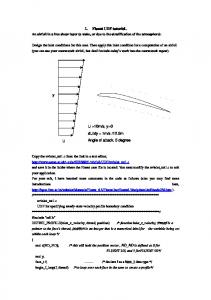
Problem Description The problem to be considered is shown schematically in Figure 1.1. A cold fluid at 20◦ C flows into the pipe through a large inlet, and mixes with a warmer fluid at 40◦ C that enters through a smaller inlet located at the elbow. The pipe dimensions are in inches, and the fluid properties and boundary conditions are given in SI units. The Reynolds number for the flow at the larger inlet is 50,800, so a turbulent flow model will be required.

Density: Viscosity: Conductivity: Specific Heat:

ρ µ k Cp

= = = =

1000 kg/m3 8 x 10 −4 Pa−s 0.677 W/m−K 4216 J/kg−K

8"

4"

Ux = 0.4 m/s T = 20oC I = 5%

1"

4" Dia. 3"

1" Dia.

8" Uy = 1.2 m/s T = 40oC I = 5%

Figure 1.1: Problem Specification

1-2



Setup and Solution Preparation 1. Download introduction.zip from the Fluent Inc. User Services Center (www.fluentusers.com) to your working folder. This file can be found by using the Documentation link on the FLUENT product page. OR, Copy introduction.zip from the FLUENT documentation CD to your working folder. For Linux / UNIX systems, you can find the file by inserting the CD into your CD-ROM drive and going to the following directory: /cdrom/fluent6.3/help/tutfiles/ where cdrom must be replaced by the name of your CD-ROM drive. For Windows systems, you can find the file by inserting the CD into your CD-ROM drive and going to the following folder: cdrom:\fluent6.3\help\tutfiles\ where cdrom must be replaced by the name of your CD-ROM drive (e.g., E). 2. Unzip introduction.zip. The file elbow.msh can be found in the introduction folder created after unzipping the file. 3. Start the 3D (3d) version of FLUENT.


1-3


Step 1: Grid 1. Read the grid file elbow.msh. File −→ Read −→Case...

(a) Select the grid file by clicking elbow.msh in the introduction folder created when you unzipped the original file. (b) Click OK to read the file and close the Select File dialog box. Note: As the grid file is read by FLUENT, messages will appear in the console that report the progress of the conversion. FLUENT will report that 13,852 hexahedral fluid cells have been read, along with a number of boundary faces with different zone identifiers.

1-4



2. Check the grid. Grid −→Check Grid Check Grid Check Domain Extents: x-coordinate: min (m) = -8.000000e+000, max (m) = 8.000000e+000 y-coordinate: min (m) = -9.134633e+000, max (m) = 8.000000e+000 z-coordinate: min (m) = 0.000000e+000, max (m) = 2.000000e+000 Volume statistics: minimum volume (m3): 5.098261e-004 maximum volume (m3): 2.330738e-002 total volume (m3): 1.607154e+002 Face area statistics: minimum face area (m2): 4.865882e-003 maximum face area (m2): 1.017924e-001 Checking number of nodes per cell. Checking number of faces per cell. Checking thread pointers. Checking number of cells per face. Checking face cells. Checking bridge faces. Checking right-handed cells. Checking face handedness. Checking face node order. Checking element type consistency. Checking boundary types: Checking face pairs. Checking periodic boundaries. Checking node count. Checking nosolve cell count. Checking nosolve face count. Checking face children. Checking cell children. Checking storage. Done.

Note: The minimum and maximum values may vary slightly when running on different platforms. The grid check will list the minimum and maximum x and y values from the grid in the default SI unit of meters, and will report a number of other grid features that are checked. Any errors in the grid will be reported at this time. In particular, you should always make sure that the minimum volume is not negative, since FLUENT cannot begin a calculation


1-5


when this is the case. In the next step, you will scale the grid so that it is in the correct unit of inches. 3. Scale the grid. Grid −→Scale...

(a) Select inches from the Grid Was Created In drop-down list in the Unit Conversion group box, by first clicking the down-arrow button and then clicking the in item from the list that appears. (b) Click Scale to scale the grid.

!

Be sure to click the Scale button only once.

The reported values of the Domain Extents will be reported in the default SI unit of meters. (c) Click the Change Length Units button to set inches as the working unit for length. (d) Confirm that the domain extents are as shown in the previous panel. (e) Close the Scale Grid panel by clicking Close. The grid is now sized correctly, and the working unit for length has been set to inches. Note: Because the default SI units will be used for everything except length, there will be no need to change any other units in this problem. The choice of inches for the unit of length has been made by the actions you have just taken. If you wanted the working unit for length to be something other than inches

1-6



(e.g., millimeters), you would have to open the Set Units panel from the Define pull-down menu and make the appropriate change. 4. Display the grid (Figure 1.2). Display −→Grid...

(a) Retain the default selection of all the items in the Surfaces selection list except default-interior. Note: A list item is selected if it is highlighted, and deselected if it is not highlighted. You can select and deselect items by clicking on the text. (b) Click Display to open a graphics window and display the grid. (c) Close the Grid Display panel. Extra: You can use the right mouse button to probe for grid information in the graphics window. If you click the right mouse button on any node in the grid, information will be displayed in the FLUENT console about the associated zone, including the name of the zone. This feature is especially useful when you have several zones of the same type and you want to distinguish between them quickly. For this 3D problem, you can make it easier to probe particular nodes by changing the view. You can perform any of the following actions in the graphics window: • Rotate the view. Drag the mouse while pressing the left mouse button. Release the mouse button when the viewing angle is satisfactory.


1-7


• Translate the view. Click the middle mouse button once at any point in the display to center the view at that point. • Zoom in to magnify a portion of the display. Drag the mouse to the right and either up or down while pressing the middle mouse button. This action will cause a white rectangle to appear in the display. When you release the mouse button, a new view will be displayed which consists entirely of the contents of the white rectangle. • Zoom out to reduce the magnification. Drag the mouse to the left and either up or down while pressing the middle mouse button. This action will cause a white rectangle to appear in the display. When you release the mouse button, the magnification of the view will be reduced by an amount that is inversely proportional to the size of the white rectangle. The new view will be centered at the center of the white rectangle.

Y Z

X

Grid FLUENT 6.3 (3d, pbns, lam)

Figure 1.2: The Hexahedral Grid for the Mixing Elbow

1-8



Step 2: Models 1. Retain the default solver settings. Define −→ Models −→Solver...

(a) Retain all of the default settings. (b) Click OK to close the Solver panel.


1-9


2. Turn on the k- turbulence model. Define −→ Models −→Viscous...

(a) Select k-epsilon from the Model list by clicking the radio button or the text, so that a black dot appears in the radio button. The Viscous Model panel will expand. (b) Select Realizable from the k-epsilon Model list. (c) Click OK to accept the model and close the Viscous Model panel.

1-10



3. Enable heat transfer by activating the energy equation. Define −→ Models −→Energy...

(a) Enable the Energy Equation option by clicking the check box or the text. Note: An option is enabled when there is a check mark in the check box, and disabled when the check box is empty. (b) Click OK to close the Energy panel.

Step 3: Materials 1. Create a new material called water. Define −→Materials...


1-11


(a) Enter water for Name by double-clicking in the text-entry box under Name and typing with the keyboard. (b) Enter the following values in the Properties group box: Property Value Density 1000 kg/m3 Cp 4216 J/kg − K Thermal Conductivity 0.677 W/m − K Viscosity 8e-04 kg/m − s (c) Click Change/Create. A Question dialog box will open, asking if you want to overwrite air. Click No so that the new material water is added to the list of materials which originally contained only air.

Extra: You could have copied the material water-liquid [h2o] from the materials database (accessed by clicking the Fluent Database... button). If the properties in the database are different from those you wish to use, you can edit the values in the Properties group box in the Materials panel and click Change/Create to update your local copy (the database copy will not be affected). (d) Make sure that there are now two materials defined locally by examining the Fluent Fluid Materials drop-down list. (e) Close the Materials panel.

1-12



Step 4: Boundary Conditions Define −→Boundary Conditions...

1. Set the boundary conditions for the fluid (fluid). (a) Select fluid from the Zone selection list.


1-13


(b) Click Set... to open the Fluid panel.

i. Select water from the Material Name drop-down list. ii. Click OK to close the Fluid panel. You have just specified water as the working fluid for this simulation. 2. Set the boundary conditions at the cold inlet (velocity-inlet-5). Hint: If you are unsure of which inlet zone corresponds to the cold inlet, you can probe the grid display with the right mouse button as described in a previous step. Not only will information be displayed in the FLUENT console, but the zone you probed will automatically be selected from the Zone selection list in the Boundary Conditions panel. (a) Select velocity-inlet-5 from the Zone selection list.

1-14



(b) Click Set... to open the Velocity Inlet panel.

i. Select Components from the Velocity Specification Method drop-down list. The Velocity Inlet panel will expand. ii. Enter 0.4 m/s for X-Velocity. iii. Retain the default value of 0 m/s for both Y-Velocity and Z-Velocity. iv. Select Intensity and Hydraulic Diameter from the Specification Method dropdown list in the Turbulence group box. v. Enter 5% for Turbulent Intensity. vi. Enter 4 inches for Hydraulic Diameter. The hydraulic diameter Dh is defined as: Dh =

4A Pw

where A is the cross-sectional area and Pw is the wetted perimeter.


1-15


vii. Click the Thermal tab.

viii. Enter 293.15 K for Temperature. ix. Click OK to close the Velocity Inlet panel. 3. In a similar manner, set the boundary conditions at the hot inlet (velocity-inlet-6), using the values in the following table: Velocity Specification Method X-Velocity Y-Velocity Z-Velocity Specification Method Turbulent Intensity Hydraulic Diameter Temperature

1-16

Components 0 m/s 1.2 m/s 0 m/s Intensity & Hydraulic Diameter 5% 1 inch 313.15 K



4. Set the boundary conditions at the outlet (pressure-outlet-7), as shown in the following panel.

Note: FLUENT will use the backflow conditions only if the fluid is flowing into the computational domain through the outlet. Since backflow might occur at some point during the solution procedure, you should set reasonable backflow conditions to prevent convergence from being adversely affected.


1-17

Introduction to Using FLUENT: Fluid Flow and Heat Transfer in a Mixing Elbow 5. For the wall of the pipe (wall), retain the default value of 0 W/m2 for Heat Flux in the Thermal tab.

6. Close the Boundary Conditions panel.

1-18



Step 5: Solution 1. Initialize the flow field, using the boundary conditions settings at the cold inlet (velocity-inlet-5) as a starting point. Solve −→ Initialize −→Initialize...

(a) Select velocity-inlet-5 from the Compute From drop-down list. (b) Enter 1.2 m/s for Y Velocity in the Initial Values group box. Note: While an initial X Velocity is an appropriate guess for the horizontal section, the addition of a Y Velocity component will give rise to a better initial guess throughout the entire elbow. (c) Click Init and close the Solution Initialization panel.


1-19


2. Enable the plotting of residuals during the calculation. Solve −→ Monitors −→Residual...

(a) Enable Plot in the Options group box. (b) Enter 1e-05 for the Absolute Criteria of continuity, as shown in the previous panel. (c) Click OK to close the Residual Monitors panel. Note: By default, all variables will be monitored and checked by FLUENT as a means to determine the convergence of the solution. Although residuals are useful for checking convergence, a more reliable method is to define a surface monitor. You will do this in the next step.

1-20



3. Define a surface monitor at the outlet (pressure-outlet-7). Solve −→ Monitors −→Surface...

(a) Set Surface Monitors to 1 by clicking once on the up-arrow button. (b) Enable the Plot and Write options for monitor-1. (c) Set Every to 3 for monitor-1. This setting instructs FLUENT to update the plot of the surface monitor and write data to a file after every 3 iterations during the solution. (d) Click the Define... button to open the Define Surface Monitor panel.

i. Select Mass-Weighted Average from the Report Type drop-down list. ii. Retain the default entry of monitor-1.out for File Name.


1-21


iii. Select Temperature... and Static Temperature from the Report of dropdown lists. iv. Select pressure-outlet-7 from the Surfaces selection list. v. Click OK to close the Define Surface Monitor panel. (e) Click OK to close the Surface Monitors panel. 4. Save the case file (elbow1.cas.gz). File −→ Write −→Case...

(a) (optional) Indicate the folder in which you would like the file to be saved. By default, the file will be saved in the folder from which you read in elbow.msh (i.e., the introduction folder). You can indicate a different folder by browsing to it or by creating a new folder. (b) Enter elbow1.cas.gz for Case File. Adding the extension .gz to the end of the file name extension instructs FLUENT to save the file in a compressed format. You do not have to include .cas in the extension (e.g., if you enter elbow1.gz, FLUENT will automatically save the file as elbow1.cas.gz). The .gz extension can also be used to save data files in a compressed format. (c) Make sure that the default Write Binary Files option is enabled, so that a binary file will be written.

1-22



(d) Click OK to close the Select File dialog box. Note: If you retained the default introduction folder in the Select File dialog box, a Warning dialog box will open to alert you that the file elbow1.cas.gz already exists. All of the files you will be instructed to save in this tutorial already exist in the introduction folder, and can be overwritten. Click OK in the Warning dialog box to proceed.

5. Start the calculation by requesting 150 iterations. Solve −→Iterate...

(a) Enter 150 for Number of Iterations. (b) Click Iterate.


1-23


Note: By starting the calculation, you are also starting to save the surface monitor data at the rate specified in the Surface Monitors panel. If a file already exists in your working folder with the name you specified in the Define Surface Monitor panel, then a Question dialog box will open, asking if you would like append the new data to the existing file. Click No in the Question dialog box, and then click OK in the Warning dialog box that follows to overwrite the existing file.

As the calculation progresses, the residuals will be plotted in the graphics window (Figure 1.3). An additional graphics window will open to display the convergence history of the mass-weighted average temperature (Figure 1.4). The solution will reach convergence after approximately 140 iterations. Note: The number of iterations required for convergence varies according to the platform used. Also, since the residual values are different for different computers, the plot that appears on your screen may not be exactly the same as the one shown here. (c) Close the Iterate panel when the calculation is complete.

1-24



Residuals continuity x-velocity y-velocity z-velocity energy k epsilon

1e+01 1e+00 1e-01 1e-02 1e-03 1e-04 1e-05 1e-06 1e-07 0

Y Z

20

40

60

80

100

120

140

Iterations

X

Scaled Residuals FLUENT 6.3 (3d, pbns, rke)

Figure 1.3: Residuals for the First 140 Iterations

monitor-1 296.6000

296.5000

296.4000

Mass 296.3000 Weighted Average (k) 296.2000 296.1000

296.0000 0

Y Z

X

20

40

60

80

100

120

140

Iteration

Convergence history of Static Temperature on pressure-outlet-7 FLUENT 6.3 (3d, pbns, rke)

Figure 1.4: Convergence History of the Mass-Weighted Average Temperature


1-25


6. Examine the plots for convergence (Figures 1.3 and 1.4). Note: There are no universal metrics for judging convergence. Residual definitions that are useful for one class of problem are sometimes misleading for other classes of problems. Therefore it is a good idea to judge convergence not only by examining residual levels, but also by monitoring relevant integrated quantities and checking for mass and energy balances. When evaluating whether convergence has been reached, there are three indicators: • The residuals have decreased to a sufficient degree. The solution has converged when the Convergence Criterion for each variable has been reached. The default criterion is that each residual will be reduced to a value of less than 10−3 , except the energy residual, for which the default criterion is 10−6 . • The solution no longer changes with more iterations. Sometimes the residuals may not fall below the convergence criterion set in the case setup. However, monitoring the representative flow variables through iterations may show that the residuals have stagnated and do not change with further iterations. This could also be considered as convergence. • The overall mass, momentum, energy, and scalar balances are obtained. You can examine the overall mass, momentum, energy and scalar balances in the Flux Reports panel. The net imbalance should be less than 0.2% of the net flux through the domain when the solution has converged. In the next step you will check to see if the mass balance indicates convergence.

1-26



7. Examine the mass flux report for convergence. Report −→Fluxes...

(a) Select pressure-outlet-7, velocity-inlet-5, and velocity-inlet-6 from the Boundaries selection list. (b) Click Compute. The sum of the flux for the inlets should be very close to the sum of the flux for the outlets. The difference will be displayed in the lower right field under kg/s, as well as in the console. Note that the imbalance is well below the 0.2% criteria suggested previously. (c) Close the Flux Reports panel. 8. Save the data file (elbow1.dat.gz). File −→ Write −→Data... In later steps of this tutorial you will save additional case and data files with different prefixes.


1-27


Step 6: Displaying the Preliminary Solution 1. Display filled contours of velocity magnitude on the symmetry plane (Figure 1.5). Display −→ Contours...

(a) Enable Filled in the Options group box. (b) Make sure that Node Values is enabled in the Options group box. (c) Select Velocity... and Velocity Magnitude from the Contours of drop-down lists. (d) Select symmetry from the Surfaces selection list. (e) Click Display to display the contours in the graphics window. Extra: Clicking the right mouse button on a point in the displayed domain will cause the value of the corresponding contour to be reported in the console.

1-28



1.42e+00 1.35e+00 1.28e+00 1.21e+00 1.14e+00 1.07e+00 9.95e-01 9.24e-01 8.53e-01 7.82e-01 7.11e-01 6.40e-01 5.69e-01 4.98e-01 4.26e-01 3.55e-01 2.84e-01 2.13e-01 1.42e-01 7.11e-02 0.00e+00

Y Z

X

Contours of Velocity Magnitude (m/s) FLUENT 6.3 (3d, pbns, rke)

Figure 1.5: Predicted Velocity Distribution after the Initial Calculation

2. Display filled contours of temperature on the symmetry plane (Figure 1.6). Display −→Contours...

(a) Select Temperature... and Static Temperature from the Contours of drop-down lists.


1-29


(b) Click Display and close the Contours panel.

3.13e+02 3.12e+02 3.11e+02 3.10e+02 3.09e+02 3.08e+02 3.07e+02 3.06e+02 3.05e+02 3.04e+02 3.03e+02 3.02e+02 3.01e+02 3.00e+02 2.99e+02 2.98e+02 2.97e+02 2.96e+02 2.95e+02 2.94e+02 2.93e+02

Y Z

X

Contours of Static Temperature (k) FLUENT 6.3 (3d, pbns, rke)

Figure 1.6: Predicted Temperature Distribution after the Initial Calculation

1-30



3. Display velocity vectors on the symmetry plane (Figures 1.7 and 1.8). Display −→ Vectors...

(a) Select symmetry from the Surfaces selection list. (b) Click Display to plot the velocity vectors. Note: The Auto Scale option is enabled by default in the Options group box. This scaling sometimes creates vectors that are too small or too large in the majority of the domain. (c) Enter 4 for Scale to increase the display size of the vectors. (d) Set Skip to 2 to make the individual vectors easier to see. (e) Click Display again (Figure 1.7). (f) Zoom in on the vectors in the display. To do this, drag your mouse to the right and either up or down, while pressing the middle mouse button. A rectangle will appear on the screen. Make sure that the rectangle frames the region that you wish to enlarge and let go of the middle mouse button. The image will be redisplayed at a higher magnification (Figure 1.8).


1-31


1.48e+00 1.42e+00 1.35e+00 1.29e+00 1.23e+00 1.17e+00 1.11e+00 1.05e+00 9.85e-01 9.24e-01 8.62e-01 8.01e-01 7.39e-01 6.77e-01 6.16e-01 5.54e-01 4.93e-01 4.31e-01 3.69e-01 3.08e-01 2.46e-01

Y Z

X

Velocity Vectors Colored By Velocity Magnitude (m/s) FLUENT 6.3 (3d, pbns, rke)

Figure 1.7: Resized Velocity Vectors

1.48e+00 1.42e+00 1.35e+00 1.29e+00 1.23e+00 1.17e+00 1.11e+00 1.05e+00 9.85e-01 9.24e-01 8.62e-01 8.01e-01 7.39e-01 6.77e-01 6.16e-01 5.54e-01 4.93e-01 4.31e-01 3.69e-01 3.08e-01 2.46e-01

Y Z

X

Velocity Vectors Colored By Velocity Magnitude (m/s) FLUENT 6.3 (3d, pbns, rke)

Figure 1.8: Magnified View of Velocity Vectors

1-32



(g) Zoom out to the original view. To do this, drag your mouse to the left and either up or down, while pressing the middle mouse button. A rectangle will appear on the screen. Make sure that the rectangle is approximately the same size as the rectangle you made while zooming in, and then let go of the middle mouse button. The image will be redisplayed at a lower magnification (Figure 1.7). If the resulting image is not centered, you can translate the view by clicking once with the middle mouse button near the center of the geometry. Alternatively, you can select the original view in the Views panel. Simply select front from the Views selection list and click Apply, as shown in the following panel. Display −→Views...

(h) Close the Vectors panel.


1-33


4. Create a line surface at the centerline of the outlet. Surface −→Iso-Surface...

(a) Select Grid... and Z-Coordinate from the Surface of Constant drop-down lists. (b) Click Compute. The range of values in the z direction will be displayed in the Min and Max fields. (c) Retain the default value of 0 inches for Iso-Values. (d) Select pressure-outlet-7 from the From Surface selection list. (e) Enter z=0 outlet for New Surface Name. (f) Click Create. After the line surface z=0 outlet is created, a new entry will automatically be generated for New Surface Name, in case you would like to create another surface. (g) Close the Iso-Surface panel.

1-34



5. Display and save an XY plot of the temperature profile across the centerline of the outlet for the initial solution (Figure 1.9). Plot −→ XY Plot...

(a) Select Temperature... and Static Temperature from the Y Axis Function dropdown lists. (b) Select z=0 outlet from the Surfaces selection list. (c) Click Plot. (d) Enable Write to File in the Options group box. The button that was originally labeled Plot will change to Write.... (e) Click Write... to open the Select File dialog box. i. Enter outlet temp1.xy for XY File. ii. Click OK to save the temperature data and close the Select File dialog box. (f) Close the Solution XY Plot panel.


1-35


z=0_outlet2 3.02e+02 3.01e+02 3.00e+02 2.99e+02 2.98e+02

Static Temperature 2.97e+02 (k) 2.96e+02 2.95e+02 2.94e+02 2.93e+02 3.5

Y Z

4

4.5

X

5

5.5

6

6.5

7

7.5

8

Position (in)

Static Temperature FLUENT 6.3 (3d, pbns, rke)

Figure 1.9: Outlet Temperature Profile for the Initial Solution

6. Define a custom field function for the dynamic head formula (ρ|V |2 /2). Define −→ Custom Field Functions...

(a) Select Density... and Density from the Field Functions drop-down lists, and click the Select button to add density to the Definition field. (b) Click the X button to add the multiplication symbol to the Definition field. (c) Select Velocity... and Velocity Magnitude from the Field Functions drop-down lists, and click the Select button to add |V| to the Definition field.

1-36



(d) Click y^x to raise the last entry in the Definition field to a power, and click 2 for the power. (e) Click the / button to add the division symbol to the Definition field, and then click 2. (f) Enter dynamic-head for New Function Name. (g) Click Define and close the Custom Field Function Calculator panel. 7. Display filled contours of the custom field function (Figure 1.10). Display −→ Contours...

(a) Select Custom Field Functions... and dynamic-head from the Contours of dropdown lists. Hint: Custom Field Functions... is at the top of the upper Contours of dropdown list. After you have opened the drop-down list, scroll up by clicking the up-arrow button on the scroll bar on the right. (b) Make sure that symmetry is selected from the Surfaces selection list. (c) Click Display and close the Contours panel. Note: You may need to change the view by zooming out after the last vector display, if you have not already done so.


1-37



Y Z

X

Contours of dynamic-head FLUENT 6.3 (3d, pbns, rke)

Figure 1.10: Contours of the Dynamic Head Custom Field Function

8. Save the settings for the custom field function by writing the case and data files (elbow1.cas.gz and elbow1.dat.gz). File −→ Write −→Case & Data... (a) Make sure that elbow1.cas.gz is entered for Case/Data File. Note: When you write the case and data file at the same time, it does not matter whether you specify the file name with a .cas or .dat extension, as both will be saved. (b) Click OK to close the Select File dialog box.

1-38



Step 7: Enabling Second-Order Discretization The elbow solution computed in the first part of this tutorial uses first-order discretization. The resulting solution is very diffusive; mixing is overpredicted, as can be seen in the contour plots of temperature and velocity distribution. You will now change to second-order discretization for all listed equations, in order to improve the accuracy of the solution. With the second-order discretization, you will change the gradient option in the solver from cell-based to node-based in order to optimize energy conservation. 1. Change the solver settings. Define −→ Models −→ Solver...

(a) Select Green-Gauss Node Based from the Gradient Option list. Note: This option is more suitable than the cell-based gradient option for unstructured meshes, as it will ensure better energy conservation. (b) Click OK to close the Solver panel.


1-39


2. Enable the second-order scheme for the calculation of all the listed equations. Solve −→ Controls −→Solution...

(a) Retain the default values in the Under-Relaxation Factors group box. (b) Select Second Order from the Pressure drop-down list in the Discretization group box. (c) Select Second Order Upwind from the Momentum, Turbulent Kinetic Energy, Turbulent Dissipation Rate, and Energy drop-down lists. Note: Scroll down the Discretization group box to find Energy. (d) Click OK to close the Solution Controls panel. 3. Continue the calculation by requesting 150 more iterations. Solve −→ Iterate...

1-40



Extra: To save the convergence history of the surface monitor for this set of iterations as a separate output file, you would need to change the File Name in the Define Surface Monitor to monitor-2.out prior to running the calculation. (a) Make sure that 150 is entered for Number of Iterations. (b) Click Iterate and close the Iterate panel when the calculation is complete. The solution will converge in approximately 57 additional iterations (Figure 1.11). The convergence history is shown in Figure 1.12.


1e+00 1e-01 1e-02 1e-03 1e-04 1e-05 1e-06 1e-07 0

Y Z

X

20

40

60

80

100

120

140

160

180

200

Iterations


Figure 1.11: Residuals for the Second-Order Energy Calculation

Note: You should expect to see the residuals jump whenever you change the solution control parameters.


1-41


monitor-1 296.6000 296.5500 296.5000 296.4500 296.4000

Mass 296.3500 Weighted Average 296.3000 (k) 296.2500 296.2000 296.1500 296.1000 0

Y Z

20

X

40

60

80

100

120

140

160

180

200

Iteration


Figure 1.12: Convergence History of Mass-Weighted Average Temperature

4. Save the case and data files for the second-order solution (elbow2.cas.gz and elbow2.dat.gz). File −→ Write −→Case & Data... (a) Enter elbow2.gz for Case/Data File. (b) Click OK to close the Select File dialog box. The files elbow2.cas.gz and elbow2.dat.gz will be saved in your folder.

1-42



5. Examine the revised temperature distribution (Figure 1.13). Display −→ Contours...

(a) Make sure that Filled is enabled in the Options group box. (b) Select Temperature... and Static Temperature from the Contours of drop-down lists. (c) Make sure that symmetry is selected from the Surfaces selection list. (d) Click Display and close the Contours panel. Figure 1.13 shows the thermal spreading of the warm fluid layer near the outer wall of the bend. Compare Figure 1.13 with Figure 1.6 to see the effects of second-order discretization.


1-43



Y Z

X


Figure 1.13: Temperature Contours for the Second-Order Solution

6. Display and save an XY plot of the temperature profile across the centerline of the outlet for the second-order solution (Figure 1.14). Plot −→ XY Plot...

(a) Disable Write to File in the Options group box by clicking the check box or the text. The button that was labeled Write... will change to Plot.

1-44



(b) Make sure that Temperature... and Static Temperature are selected from the Y Axis Function drop-down lists. (c) Make sure that z=0 outlet is selected from the Surfaces selection list. (d) Click Plot.

z=0_outlet 3.00e+02 2.99e+02 2.98e+02 2.97e+02

Static Temperature 2.96e+02 (k) 2.95e+02 2.94e+02 2.93e+02 3.5

Y Z

4

4.5

5

X

5.5

6

6.5

7

7.5

8

Position (in)


Figure 1.14: Outlet Temperature Profile for the Second-Order Solution (e) Enable Write to File in the Options group box. The button that was labeled Plot will change to Write.... (f) Click Write... to open the Select File dialog box. i. Enter outlet temp2.xy for XY File. ii. Click OK to save the temperature data. (g) Close the Solution XY Plot panel.


1-45


Step 8: Adapting the Grid The elbow solution can be improved further by refining the grid to better resolve the flow details. In the following steps, you will adapt the grid based on the temperature gradients in the current solution. Once the grid has been refined, you will continue the calculation. 1. Adapt the grid in the regions of high temperature gradient. Adapt −→Gradient...

(a) Make sure that Refine is enabled in the Options group box. It is not necessary to deselect Coarsen in this instance, since FLUENT will not coarsen beyond the original mesh for a 3D grid. (b) Select Temperature... and Static Temperature from the Gradients of drop-down lists. (c) Click Compute. FLUENT will update the Min and Max values to show the minimum and maximum temperature gradient. (d) Enter 0.003 for Refine Threshold. It is a good rule of thumb to use 10% of the maximum gradient when setting the value for Refine Threshold. (e) Click Mark. FLUENT will report in the console that approximately 1258 cells were marked for adaption.

1-46



(f) Click the Manage... button to open the Manage Adaption Registers panel.

i. Click Display. FLUENT will display the cells marked for adaption in the graphics window (Figure 1.15).

Y Z

X

Adaption Markings (gradient-r0) FLUENT 6.3 (3d, pbns, rke)

Figure 1.15: Cells Marked for Adaption


1-47


Extra: You can change the way FLUENT displays cells marked for adaption (Figure 1.16) by performing the following steps: A. Click the Options... button in the Manage Adaption Registers panel to open the Adaption Display Options panel.

B. Enable Draw Grid in the Options group box. The Grid Display panel will open.

C. Make sure that Edges is the only option enabled in the Options group box. D. Select Feature from the Edge Type list. E. Select all of the items except default-interior from the Surfaces selection list. F. Click Display and close the Grid Display panel.

1-48



G. Enable Filled in the Options group box in the Adaption Display Options panel. H. Enable Wireframe in the Refine group box. I. Click OK to close the Adaption Display Options panel. J. Click Display in the Manage Adaption Registers panel. K. Rotate the view and zoom in to get the display shown in Figure 1.16.

Y XZ

Adaption Markings (gradient-r0) FLUENT 6.3 (3d, pbns, rke)

Figure 1.16: Alternate Display of Cells Marked for Adaption L. After you are finished viewing the marked cells, rotate the view back and zoom out again to return to the angle and magnification shown in Figure 1.13. ii. Click Adapt in the Manage Adaption Registers panel. A Question dialog box will open, asking whether it is acceptable to adapt the grid by creating hanging nodes. Click Yes to proceed.

Note: There are two different ways to adapt. You can click Adapt in the Manage Adaption Registers panel as was just done, or close this panel and perform the adaption using the Gradient Adaption panel. If


1-49


you use the Adapt button in the Gradient Adaption panel, FLUENT will recreate an adaption register. Therefore, once you have the Manage Adaption Registers panel open, it saves time to use the Adapt button there. iii. Close the Manage Adaption Registers panel. (g) Close the Gradient Adaption panel. 2. Display the adapted grid (Figure 1.17). Display −→Grid...

(a) Make sure that All is selected from the Edge Type list. (b) Deselect all of the highlighted items from the Surfaces selection list except for symmetry. (c) Click Display and close the Grid Display panel.

1-50



Y Z

X

Grid FLUENT 6.3 (3d, pbns, rke)

Figure 1.17: The Adapted Grid

3. Request an additional 150 iterations. Solve −→ Iterate...

The solution will converge after approximately 100 additional iterations (Figures 1.18 and 1.19). 4. Save the case and data files for the second-order solution with an adapted grid (elbow3.cas.gz and elbow3.dat.gz). File −→ Write −→ Case & Data... (a) Enter elbow3.gz for Case/Data File. (b) Click OK to close the Select File dialog box. The files elbow3.cas.gz and elbow3.dat.gz will be saved in your folder.


1-51



1e+00 1e-01 1e-02 1e-03 1e-04 1e-05 1e-06 1e-07 0

Y Z

50

100

150

200

250

300

Iterations

X


Figure 1.18: The Complete Residual History

monitor-1 296.6000 296.5500 296.5000 296.4500 296.4000

Mass 296.3500 Weighted Average 296.3000 (k) 296.2500 296.2000 296.1500 296.1000 0

Y Z

X

50

100

150

200

250

300

Iteration


Figure 1.19: Convergence History of Mass-Weighted Average Temperature

1-52



5. Examine the filled temperature distribution (using node values) on the revised grid (Figure 1.20). Display −→ Contours...


Y Z

X


Figure 1.20: Filled Contours of Temperature Using the Adapted Grid 6. Display and save an XY plot of the temperature profile across the centerline of the outlet for the adapted second-order solution (Figure 1.21). Plot −→ XY Plot...


1-53


(a) Disable Write to File in the Options group box. The button that was originally labeled Write... will change to Plot. (b) Make sure that Temperature... and Static Temperature are selected from the Y Axis Function drop-down lists. (c) Make sure that z=0 outlet is selected from the Surfaces selection list. (d) Click Plot.

z=0_outlet 3.00e+02 2.99e+02 2.98e+02 2.97e+02

Static Temperature 2.96e+02 (k) 2.95e+02 2.94e+02 2.93e+02 3.5

Y Z

4

4.5

5

X

5.5

6

6.5

7

7.5

8

Position (in)


Figure 1.21: Outlet Temperature Profile for the Adapted Second-Order Solution (e) Enable Write to File in the Options group box. The button that was originally labeled Plot will change to Write.... (f) Click Write... to open the Select File dialog box. i. Enter outlet temp3.xy for XY File. ii. Click OK to save the temperature data. (g) Close the Solution XY Plot panel.

1-54



7. Display the outlet temperature profiles for each of the three solutions on a single plot (Figure 1.22). Plot −→File...

(a) Click the Add... button to open the Select File dialog box.


1-55


i. Click once on outlet temp1.xy, outlet temp2.xy, and outlet temp3.xy. Each of these files will be listed with their folder in the XY File(s) list to indicate that they have been selected. Hint: If you select a file by mistake, simply click the file in the XY File(s) list and then click Remove. ii. Click OK to close the Select File dialog box. (b) Select the folder path ending in outlet temp1.xy from the Files selection list. (c) Enter 1st Order Soln in the lowest field on the right (next to the Change Legend Entry button). (d) Click the Change Legend Entry button. The item in the Legend Entries list for outlet temp1.xy will be changed to 1st Order Soln. This legend entry will be displayed in the upper-left corner of the XY plot generated in a later step. (e) In a similar manner, change the legend entry for the folder path ending in outlet temp2.xy to be 2nd Order Soln. (f) In a similar manner, change the legend entry for the folder path ending in outlet temp3.xy to be Adapted Grid. (g) Click Plot and close the File XY Plot panel. Figure 1.22 shows the three temperature profiles at the centerline of the outlet. It is apparent by comparing both the shape of the profiles and the predicted outer wall temperature that the solution is highly dependent on the mesh and solution options. Specifically, further mesh adaption should be used in order to obtain a solution that is independent of the mesh. Extra: You can perform additional grid adaptions based on temperature gradient and run the calculation to see how the temperature profile changes at the outlet. A case and data file (elbow4.cas.gz and elbow4.dat.gz) has been provided in which the grid has undergone three more levels of adaption, and the resulting temperature profiles have been plotted with outlet temp2.xy and outlet temp3.xy in Figure 1.23. It is evident from Figure 1.23 that as the grid is adapted further, the profiles converge on a grid-independent profile. The resulting wall temperature at the outlet is predicted to be around 300.25 K once grid independence is achieved. If the adaption steps had not been performed, the wall temperature would have incorrectly been estimated at around 298.5 K. If computational resources allow, it is always recommended to perform successive adaptions until the solution is independent of the grid (within an acceptable tolerance). Typically, profiles of important variables are examined (in this case, temperature) and compared to determine grid independence.

1-56



Figure 1.22: Outlet Temperature Profiles for the Three Solutions

Figure 1.23: Outlet Temperature Profiles for Subsequent Grid Adaption Steps


1-57


Summary Comparison of the filled temperature contours for the first solution (using the original grid and first-order discretization) and the last solution (using an adapted grid and second-order discretization) clearly indicate that the latter is much less diffusive. While first-order discretization is the default scheme in FLUENT, it is good practice to use your first-order solution as a starting guess for a calculation that uses a higher-order discretization scheme and, optionally, an adapted grid. Note that in this problem, the flow field is decoupled from temperature, since all properties are constant. For such cases, it is more efficient to compute the flow-field solution first (i.e., without solving the energy equation) and then solve for energy (i.e., without solving the flow equations). You will use the Solution Controls panel to turn the solution of the equations on and off during this procedure.

1-58


Tutorial 2.

Modeling Periodic Flow and Heat Transfer

Introduction Many industrial applications, such as steam generation in a boiler or air cooling in the coil of an air conditioner, can be modeled as two-dimensional periodic heat flow. This tutorial illustrates how to set up and solve a periodic heat transfer problem, given a pregenerated mesh. The system that is modeled is a bank of tubes containing a flowing fluid at one temperature that is immersed in a second fluid in cross flow at a different temperature. Both fluids are water, and the flow is classified as laminar and steady, with a Reynolds number of approximately 100. The mass flow rate of the cross flow is known and the model is used to predict the flow and temperature fields that result from convective heat transfer. Due to symmetry of the tube bank and the periodicity of the flow inherent in the tube bank geometry, only a portion of the geometry will be modeled in FLUENT, with symmetry applied to the outer boundaries. The resulting mesh consists of a periodic module with symmetry. In the tutorial, the inlet boundary will be redefined as a periodic zone, and the outflow boundary defined as its shadow. This tutorial demonstrates how to do the following: • Create periodic zones. • Define a specified periodic mass flow rate. • Model periodic heat transfer with specified temperature boundary conditions. • Calculate a solution using the pressure-based solver. • Plot temperature profiles on specified isosurfaces.

Prerequisites This tutorial assumes that you are familiar with the menu structure in FLUENT and that you have completed Tutorial 1. Some steps in the setup and solution procedure will not be shown explicitly.


2-1


Problem Description This problem considers a 2D section of a tube bank. A schematic of the problem is shown in Figure 2.1. The bank consists of uniformly spaced tubes with a diameter of 1 cm, which are staggered across the cross-fluid flow. Their centers are separated by a distance of 2 cm in the x direction, and 1 cm in the y direction. The bank has a depth of 1 m. 4 cm

Τ

∞ = 300 K

⋅

m = 0.05 kg/s

{

1 cm

Τ wall = 400 K 0.5 cm

3 ρ = 998.2 kg/m µ = 0.001003 kg/m-s

c p = 4182 J/kg-K k = 0.6 W/m-K

Figure 2.1: Schematic of the Problem

Because of the symmetry of the tube bank geometry, only a portion of the domain needs to be modeled. The computational domain is shown in outline in Figure 2.1. A mass flow rate of 0.05 kg/s is applied to the inlet boundary of the periodic module. The temperature of the tube wall (Twall ) is 400 K and the bulk temperature of the cross flow water (T∞ ) is 300 K. The properties of water that are used in the model are shown in Figure 2.1.

2-2



Setup and Solution Preparation 1. Download periodic_flow_heat.zip from the Fluent Inc. User Services Center or copy it from the FLUENT documentation CD to your working folder (as described in Tutorial 1). 2. Unzip periodic_flow_heat.zip. The file tubebank.msh can be found in the periodic flow heat folder created after unzipping the file. 3. Start the 2D (2d) version of FLUENT.

Step 1: Grid 1. Read the mesh file tubebank.msh. File −→ Read −→Case... 2. Check the grid. Grid −→Check FLUENT will perform various checks on the mesh and report the progress in the console. Make sure that the minimum volume reported is a positive number. 3. Scale the grid. Grid −→Scale...

(a) Select cm (centimeters) from the Grid Was Created In drop-down list in the Unit Conversion group box. (b) Click Scale to scale the grid. (c) Close the Scale Grid panel.


2-3


4. Display the mesh (Figure 2.2). Display −→Grid...

(a) Retain the default settings. (b) Click Display and close the Grid Display panel.


Figure 2.2: Mesh for the Periodic Tube Bank

2-4



Quadrilateral cells are used in the regions surrounding the tube walls and triangular cells are used for the rest of the domain, resulting in a hybrid mesh (see Figure 2.2). The quadrilateral cells provide better resolution of the viscous gradients near the tube walls. The remainder of the computational domain is filled with triangular cells for the sake of convenience. Extra: You can use the right mouse button to probe for grid information in the graphics window. If you click the right mouse button on any node in the grid, information will be displayed in the FLUENT console about the associated zone, including the name of the zone. This feature is especially useful when you have several zones of the same type and you want to distinguish between them quickly. 5. Create the periodic zone. The inlet (wall-9) and outflow (wall-12) boundaries currently defined as wall zones need to be redefined as periodic using the text user interface. The wall-9 boundary will be redefined as a translationally periodic zone and wall-12 as a periodic shadow of wall-9. (a) Press in the console to get the command prompt (>). (b) Enter the text command and input responses outlined in boxes as shown:

> grid/modify-zones/make-periodic Periodic zone [()] 9 Shadow zone [()] 12 Rotational periodic? (if no, translational) [yes] no Create periodic zones? [yes] yes Auto detect translation vector? [yes] yes computed translation deltas: 0.040000 0.000000 all 26 faces matched for zones 9 and 12. zone 12 deleted created periodic zones.


2-5


Step 2: Models 1. Retain the default settings for the solver. Define −→ Models −→Solver...

2. Activate heat transfer. Define −→ Models −→Energy...

(a) Enable the Energy Equation option. (b) Click OK to close the Energy panel.

2-6



3. Define the periodic flow conditions. Define −→Periodic Conditions...

(a) Select Specify Mass Flow from the Type list. This will allow you to specify the Mass Flow Rate. (b) Enter 0.05 kg/s for Mass Flow Rate. (c) Click OK to close the Periodic Conditions panel.


2-7


Step 3: Materials The default properties for water defined in FLUENT are suitable for this problem. In this step, you will make sure that this material is available for selecting in future steps. 1. Add water to the list of fluid materials by copying it from the FLUENT materials database. Define −→Materials... (a) Click the Fluent Database... button to open the Fluent Database Materials panel.

i. Select water-liquid (h2o) from the Fluent Fluid Materials selection list. Scroll down the list to find water-liquid (h2o). Selecting this item will display the default properties in the panel. ii. Click Copy and close the Fluent Database Materials panel. The Materials panel will now display the copied properties for water-liquid.

2-8



(b) Close the Materials panel.


2-9



1. Set the boundary conditions for the continuum fluid zone (fluid-16).

(a) Select water-liquid from the Material Name drop-down list. (b) Click OK to close the Fluid panel.

2-10



2. Set the boundary conditions for the bottom wall of the left tube (wall-21).

(a) Enter wall-bottom for Zone Name. (b) Click the Thermal tab. i. Select Temperature from the Thermal Conditions list. ii. Enter 400 K for Temperature. These settings will specify a constant wall temperature of 400 K. (c) Click OK to close the Wall panel.


2-11


3. Set the boundary conditions for the top wall of the right tube (wall-3).

(a) Enter wall-top for Zone Name. (b) Click the Thermal tab. i. Select Temperature from the Thermal Conditions list. ii. Enter 400 K for Temperature. (c) Click OK to close the Wall panel. 4. Close the Boundary Conditions panel.

2-12



Step 5: Solution 1. Set the parameters that control the solution. Solve −→ Controls −→Solution...

(a) Enter 0.9 for Energy in the Under-Relaxation Factors group box. Scroll down to find the Energy number-entry box. (b) Select Second Order Upwind from the Momentum and Energy drop-down lists in the Discretization group box. (c) Click OK to close the Solution Controls panel.


2-13



(a) Enable Plot in the Options group box. (b) Click OK to close the Residual Monitors panel. 3. Initialize the solution. Solve −→ Initialize −→Initialize...

2-14



(a) Retain the default setting of 300 K for Temperature in the Initial Values group box. (b) Click Init and close the Solution Initialization panel. The values shown in the panel will be used as the initial condition for the solution. 4. Save the case file (tubebank.cas). File −→ Write −→Case... 5. Start the calculation by requesting 350 iterations. Solve −→Iterate...

(a) Enter 350 for Number of Iterations. (b) Click Iterate. (c) Close the Iterate panel when the calculation is complete. The energy residual curve that is displayed in the graphics window will begin to flatten out as it approaches 350 iterations. For the solution to converge to the recommended residual value of 10−6 , you need to reduce the under-relaxation factor for energy. 6. Change the Under-Relaxation Factor for Energy to 0.6. Solve −→ Controls −→Solution... 7. Continue the calculation by requesting another 300 iterations. Solve −→Iterate... After restarting the calculation, the plot of the energy residual will display an initial dip as a result of the reduction of the under-relaxation factor. The solution will converge in a total of approximately 580 iterations. 8. Save the case and data files (tubebank.cas and tubebank.dat). File −→ Write −→Case & Data...


2-15


Step 6: Postprocessing Postprocess the results and create plots and graphs of the solution. 1. Display filled contours of static pressure (Figure 2.3). Display −→Contours...

(a) Enable Filled in the Options group box. (b) Retain the default selection of Pressure... and Static Pressure from the Contours of drop-down lists. (c) Click Display and close the Contours panel.

2-16



8.18e-02 7.55e-02 6.92e-02 6.28e-02 5.65e-02 5.02e-02 4.38e-02 3.75e-02 3.12e-02 2.48e-02 1.85e-02 1.22e-02 5.82e-03 -5.20e-04 -6.85e-03 -1.32e-02 -1.95e-02 -2.59e-02 -3.22e-02 -3.85e-02 -4.49e-02

Contours of Static Pressure (pascal) FLUENT 6.3 (2d, pbns, lam)

Figure 2.3: Contours of Static Pressure

2. Change the view to mirror the display across the symmetry planes (Figure 2.4). Display −→Views...

(a) Select all of the symmetry zones (symmetry-18, symmetry-13, symmetry-11, and symmetry-24) in the Mirror Planes selection list by clicking on the shaded icon in the upper right corner. Note: There are four symmetry zones in the Mirror Planes selection list because the top and bottom symmetry planes in the domain are each comprised of two symmetry zones, one on each side of the tube centered on the


2-17


plane. It is also possible to generate the same display shown in Figure 2.4 by selecting just one of the symmetry zones on the top symmetry plane, and one on the bottom. (b) Click Apply and close the Views panel. (c) Translate the display of symmetry contours so that it is centered in the graphics window by using the left mouse button (Figure 2.4).

8.18e-02 7.55e-02 6.92e-02 6.28e-02 5.65e-02 5.02e-02 4.38e-02 3.75e-02 3.12e-02 2.48e-02 1.85e-02 1.22e-02 5.82e-03 -5.20e-04 -6.85e-03 -1.32e-02 -1.95e-02 -2.59e-02 -3.22e-02 -3.85e-02 -4.49e-02

Contours of Static Pressure (pascal) FLUENT 6.3 (2d, pbns, lam)

Figure 2.4: Contours of Static Pressure with Symmetry

The pressure contours displayed in Figure 2.4 do not include the linear pressure gradient computed by the solver. Thus, the contours are periodic at the inlet and outflow boundaries.

2-18



3. Display filled contours of static temperature (Figure 2.5). Display −→Contours...

(a) Select Temperature... and Static Temperature from the Contours of drop-down lists. (b) Click Display and close the Contours panel. The contours in Figure 2.5 reveal the temperature increase in the fluid due to heat transfer from the tubes. The hotter fluid is confined to the near-wall and wake regions, while a narrow stream of cooler fluid is convected through the tube bank.


2-19



Contours of Static Temperature (k) FLUENT 6.3 (2d, pbns, lam)

Figure 2.5: Contours of Static Temperature

2-20



4. Display the velocity vectors (Figure 2.6). Display −→Vectors...

(a) Enter 2 for the Scale. This will increase the size of the displayed vectors, making it easier to view the flow patterns. (b) Retain the default selection of Velocity from the Vectors of drop-down list. (c) Retain the default selection of Velocity... and Velocity Magnitude from the Color by drop-down lists. (d) Click Display and close the Vectors panel. (e) Zoom in on the upper right portion of one of the left tubes to get the display shown in (Figure 2.6), by using the middle mouse button in the graphics window. The magnified view of the velocity vector plot in Figure 2.6 clearly shows the recirculating flow behind the tube and the boundary layer development along the tube surface.


2-21


1.31e-02 1.25e-02 1.18e-02 1.12e-02 1.05e-02 9.85e-03 9.19e-03 8.53e-03 7.88e-03 7.22e-03 6.56e-03 5.91e-03 5.25e-03 4.60e-03 3.94e-03 3.28e-03 2.63e-03 1.97e-03 1.31e-03 6.58e-04 1.95e-06

Velocity Vectors Colored By Velocity Magnitude (m/s) FLUENT 6.3 (2d, pbns, lam)

Figure 2.6: Velocity Vectors

5. Create an isosurface on the periodic tube bank at x = 0.01 m (through the first column of tubes). This isosurface and the ones created in the steps that follow will be used for the plotting of temperature profiles. Surface −→Iso-Surface...

(a) Select Grid... and X-Coordinate from the Surface of Constant drop-down lists. (b) Enter 0.01 for Iso-Values.

2-22



(c) Enter x=0.01m for New Surface Name. (d) Click Create. 6. In a similar manner, create an isosurface on the periodic tube bank at x = 0.02 m (halfway between the two columns of tubes) named x=0.02m. 7. In a similar manner, create an isosurface on the periodic tube bank at x = 0.03 m (through the middle of the second column of tubes) named x=0.03m, and close the Iso-Surface panel. 8. Create an XY plot of static temperature on the three isosurfaces (Figure 2.7). Plot −→XY Plot...

(a) Enter 0 for X and 1 for Y in the Plot Direction group box, as shown in the previous panel. With a Plot Direction vector of (0,1), FLUENT will plot the selected variable as a function of y. Since you are plotting the temperature profile on cross sections of constant x, the temperature varies with the y direction. (b) Select Temperature... and Static Temperature from the Y-Axis Function dropdown lists. (c) Select x=0.01m, x=0.02m, and x=0.03m in the Surfaces selection list. Scroll down to find the x=0.01m, x=0.02m, and x=0.03m surfaces.


2-23


(d) Click Curves... to open the Curves - Solution XY Plot panel. This panel is used to define plot styles for the different plot curves.

i. Select + from the Symbol drop-down list. Scroll up to find the + item. ii. Click Apply to assign the + symbol to the x = 0.01 m curve. iii. Set the Curve # to 1 to define the style for the x = 0.02 m curve. iv. Select x from the Symbol drop-down list. Scroll up to find the x item. v. Enter 0.5 for Size. vi. Click Apply and close the Curves - Solution XY Plot panel. Since you did not change the curve style for the x = 0.03 m curve, the default symbol will be used. (e) Click Plot and close the Solution XY Plot panel.

2-24



x=0.01m x=0.02m x=0.03m

4.00e+02 3.80e+02 3.60e+02 3.40e+02

Static Temperature 3.20e+02 (k) 3.00e+02 2.80e+02 2.60e+02 0

0.001 0.002 0.003 0.004 0.005 0.006 0.007 0.008 0.009 0.01

Position (m)

Static Temperature FLUENT 6.3 (2d, pbns, lam)

Figure 2.7: Static Temperature at x=0.01, 0.02, and 0.03 m

Summary In this tutorial, periodic flow and heat transfer in a staggered tube bank were modeled in FLUENT. The model was set up assuming a known mass flow through the tube bank and constant wall temperatures. Due to the periodic nature of the flow and symmetry of the geometry, only a small piece of the full geometry was modeled. In addition, the tube bank configuration lent itself to the use of a hybrid mesh with quadrilateral cells around the tubes and triangles elsewhere. The Periodic Conditions panel makes it easy to run this type of model with a variety of operating conditions. For example, different flow rates (and hence different Reynolds numbers) can be studied, or a different inlet bulk temperature can be imposed. The resulting solution can then be examined to extract the pressure drop per tube row and overall Nusselt number for a range of Reynolds numbers.

Further Improvements This tutorial guides you through the steps to reach an initial solution. You may be able to obtain a more accurate solution by using an appropriate higher-order discretization scheme and by adapting the grid. Grid adaption can also ensure that the solution is independent of the grid. These steps are demonstrated in Tutorial 1.


2-25


2-26


Tutorial 3.

Modeling External Compressible Flow

Introduction The purpose of this tutorial is to compute the turbulent flow past a transonic airfoil at a nonzero angle of attack. You will use the Spalart-Allmaras turbulence model. This tutorial will demonstrate how to do the following: • Model compressible flow (using the ideal gas law for density). • Set boundary conditions for external aerodynamics. • Use the Spalart-Allmaras turbulence model. • Use Full Multigrid (FMG) initialization to obtain better initial field values. • Calculate a solution using the pressure-based coupled solver. • Use force and surface monitors to check solution convergence. • Check the near-wall grid resolution by plotting the distribution of y + .



3-1


Problem Description The problem considers the flow around an airfoil at an angle of attack α = 4◦ and a free stream Mach number of 0.8 (M∞ = 0.8). The flow is transonic, and has a fairly strong shock near the mid-chord (x/c = 0.45) on the upper (suction) side. The chord length is 1 m. The geometry of the airfoil is shown in Figure 3.1. α = 4°

M∞= 0.8 1m


Setup and Solution Preparation 1. Download external_compressible.zip from the Fluent Inc. User Services Center or copy it from the FLUENT documentation CD to your working folder (as described in Tutorial 1). 2. Unzip external_compressible.zip. The file airfoil.msh can be found in the external compressible folder created after unzipping the file. 3. Start the 2D (2d) version of FLUENT.

3-2



Step 1: Grid 1. Read the grid file airfoil.msh. File −→ Read −→Case... 2. Check the grid. Grid −→Check FLUENT will perform various checks on the mesh and will report the progress in the console. Make sure that the minimum volume reported is a positive number. 3. Display the grid (Figures 3.2 and 3.3). Display −→Grid...

(a) Retain the default settings. (b) Click Display and close the Grid Display panel. (c) Zoom in on the region around the airfoil (as shown in Figure 3.3), by using the middle mouse button in the graphics window. Quadrilateral cells were used for this simple geometry because they can be stretched easily to account for different flow gradients in different directions. In the present case, the gradients normal to the airfoil wall are much greater than those tangent to the airfoil. Consequently, the cells near the surface have high aspect ratios. For geometries that are more difficult to mesh, it may be easier to create a hybrid mesh comprised of quadrilateral and triangular cells. A parabola was chosen to represent the far-field boundary because it has no discontinuities in slope, enabling the construction of a smooth mesh in the interior of the domain.


3-3



Figure 3.2: The Entire Grid


Figure 3.3: Magnified View of the Grid Around the Airfoil

3-4



Extra: You can use the right mouse button to probe for grid information in the graphics window. If you click the right mouse button on any node in the grid, information will be displayed in the FLUENT console about the associated zone, including the name of the zone. This feature is especially useful when you have several zones of the same type and you want to distinguish between them quickly. 4. Reorder the mesh. Grid −→ Reorder −→Domain This is done to reduce the bandwidth of the cell neighbor number and to speed up the computations. This is especially important for large cases involving 1 million or more cells. The method used to reorder the domain is the Reverse Cuthill-McKee method.

Step 2: Models 1. Specify the solver settings. Define −→ Models −→Solver...

(a) Retain the default selection of Pressure Based from the Solver list. The pressure-based coupled solver is a good alternative to FLUENT’s densitybased solvers when dealing with applications involving high-speed aerodynamics with shocks. Selection of the coupled algorithm is made in the Solution Controls panel in Step 6: Solution.


3-5


(b) Select Green-Gauss Node Based from the Gradient Option list. This option uses better numerics, in particular on unstructured meshes. It also tends to predict drag more accurately. (c) Click OK to close the Solver panel. 2. Enable the Spalart-Allmaras turbulence model. Define −→ Models −→Viscous...

(a) Select the Spalart-Allmaras in the Model list. (b) Select Strain/Vorticity-Based Production in the Spalart-Allmaras Options list. (c) Retain the default settings in the Model Constants group box. (d) Click OK to close the Viscous Model panel. Note: The Spalart-Allmaras model is a relatively simple one-equation model that solves a modeled transport equation for the kinematic eddy (turbulent) viscosity. This embodies a relatively new class of one-equation models in which it is not necessary to calculate a length scale related to the local shear layer thickness. The Spalart-Allmaras model was designed specifically for aerospace applications involving wall-bounded flows and has been shown to give good results for boundary layers subjected to adverse pressure gradients.

3-6



Step 3: Materials The default Fluid Material is air, which is the working fluid in this problem. The default settings need to be modified to account for compressibility and variations of the thermophysical properties with temperature. 1. Set the properties for air, the default fluid material. Define −→Materials...

(a) Select ideal-gas from the Density drop-down list. (b) Select sutherland from the Viscosity drop-down list to open the Sutherland Law panel. Scroll down the list to find sutherland.


3-7


i. Retain the default selection of Three Coefficient Method from the Methods list. ii. Click OK to close the Sutherland Law panel. The Sutherland law for viscosity is well suited for high-speed compressible flows. (c) Click Change/Create to save these settings. (d) Close the Materials panel. While Density and Viscosity have been made temperature dependent, Cp and Thermal Conductivity have been left constant. For high-speed compressible flows, thermal dependency of the physical properties is generally recommended. For simplicity, Thermal Conductivity and Cp are assumed to be constant in this tutorial.

Step 4: Operating Conditions 1. Set the operating pressure. Define −→Operating Conditions...

(a) Retain the default entry of 101325 Pa for Operating Pressure. The operating pressure should be set to a meaningful mean value in order to avoid round-off errors. (b) Click OK to close the Operating Conditions panel. See Section 8.14 of the User’s Guide for more information on how to set the operating pressure.

3-8




1. Set the boundary conditions for pressure-far-field-1.

(a) Retain the default entry of 0 Pa for Gauge Pressure.


3-9


(b) Enter 0.8 for Mach Number. (c) Enter 0.997564 and 0.069756 for the X-Component of Flow Direction and Y-Component of Flow Direction, respectively. These values are determined by the 4◦ angle of attack: cos 4◦ ≈ 0.997564 and sin 4◦ ≈ 0.069756. (d) Select Turbulent Viscosity Ratio from the Specification Method drop-down list in the Turbulence group box. (e) Retain the default entry of 10 for Turbulent Viscosity Ratio. The viscosity ratio should be between 1 and 10 for external flows. (f) Click the Thermal tab and retain the default entry of 300 K for Temperature.

(g) Click OK to close the Pressure Far-Field panel. 2. Close the Boundary Conditions panel.

3-10



Step 6: Solution 1. Set the solution controls. Solve −→ Controls −→Solution...

(a) Select Coupled from the Pressure-Velocity Coupling drop-down list. (b) Retain the default entry of 200 for the Courant Number. (c) Enter 0.5 for Momentum and Pressure in the Explicit Relaxation Factors group box. Under-relaxing the momentum and pressure factors is recommended for higherorder discretization schemes. (d) Enter 0.5 for Density in the Under-Relaxation Factors group box. Under-relaxing the density factor is recommended for high-speed compressible flows. (e) Enter 0.9 for Modified Turbulent Viscosity. Larger under-relaxation factors (i.e., closer to 1) will generally result in faster convergence. However, instability can arise that may need to be eliminated by decreasing the under-relaxation factors. (f) Retain the default selection of Standard from the Pressure drop-down list in the Discretization group box. (g) Select Second Order Upwind from the Density, Momentum, Modified Turbulent Viscosity, and Energy drop-down lists. Scroll down to find the Energy drop-down list. The second-order scheme will resolve the boundary layer and shock more accurately than the first-order scheme.


3-11


(h) Click OK to accept the settings and close the Solution Controls panel. 2. Initialize the solution. Solve −→ Initialize −→Initialize...

(a) Select pressure-far-field-1 in the Compute From drop-down list. (b) Click Init to initialize the solution. (c) Close the Solution Initialization panel. 3. Run the Full Multigrid (FMG) initialization. FMG initialization often facilitates an easier start-up, where no CFL ramping is necessary, thereby reducing the number of iterations for convergence. (a) Press in the console to get the command prompt (>). (b) Enter the text commands and input responses outlined in boxes as shown, accepting the default values by pressing when no input response is given: > solve/initialize/set-fmg-initialization Customize your FMG initialization: set the number of multigrid levels [5] set FMG parameters on levels .. residual reduction on level 1 is: [0.001] number of cycles on level 1 is: [10] 100

3-12



residual reduction on level 2 is: [0.001] number of cycles on level 2 is: [50] 100 residual reduction on level 3 is: [0.001] number of cycles on level 3 is: [100] residual reduction on level 4 is: [0.001] number of cycles on level 4 is: [500] residual reduction on level 5 [coarsest grid] is: number of cycles on level 5 is: [500]

[0.001]

Number of FMG (and FAS geometric multigrid) levels: 5 * FMG customization summary: * residual reduction on level 0 [finest grid] is: 0.001 * number of cycles on level 0 is: 1 * residual reduction on level 1 is: 0.001 * number of cycles on level 1 is: 100 * residual reduction on level 2 is: 0.001 * number of cycles on level 2 is: 100 * residual reduction on level 3 is: 0.001 * number of cycles on level 3 is: 100 * residual reduction on level 4 is: 0.001 * number of cycles on level 4 is: 500 * residual reduction on level 5 [coarsest grid] is: 0.001 * number of cycles on level 5 is: 500 * FMG customization complete set FMG courant-number [0.75] enable FMG verbose? [no] yes > solve/initialize/fmg-initialization Enable FMG initialization? [no] yes

Note: The FMG initialized flow field can be inspected using FLUENT’s postprocessing tools. 4. Save the case and data files (airfoil.cas and airfoil.dat). File −→ Write −→Case & Data... It is good practice to save the case and data files during several stages of your case setup. 5. Start the calculation by requesting 50 iterations. Solve −→Iterate...


3-13


(a) Enter 50 for Number of Iterations. (b) Click Iterate. (c) Close the Iterate panel when the calculation is complete. By performing some iterations before setting up the force monitors, you will avoid large initial transients in the monitor plots. This will reduce the axes range and make it easier to judge the convergence. 6. Define a force monitor to plot and write the drag coefficient for the walls of the airfoil. Solve −→ Monitors −→Force...

(a) Enable Plot in the Options group box. (b) Enable the Write option to save the monitor history to a file. Note: If you do not select the Write option, the history information will be lost when you exit FLUENT. (c) Retain the default selection of Drag from the Coefficient drop-down list. (d) Retain the default entry of cd-history for the File Name. (e) Select wall-bottom and wall-top from the Wall Zones selection list. (f) Enter 0.9976 for X and 0.06976 for Y in the Force Vector group box. These X and Y values ensure that the drag coefficient is calculated parallel to the free-stream flow, which is 4◦ off of the global coordinates. (g) Set the Plot Window to 1. (h) Click Apply.

3-14



7. In a similar manner, define a force monitor for the lift coefficient, as shown in the following panel. Click Apply after the settings are complete. Solve −→ Monitors −→Force...

The X and Y values shown ensure that the lift coefficient is calculated normal to the free-stream flow, which is 4◦ off of the global coordinates. 8. In a similar manner, define a force monitor for the moment coefficient, as shown in the following panel. Click Apply after the settings are complete and close the Force Monitors panel. Solve −→ Monitors −→Force...


3-15


9. Set the reference values that are used to compute the lift, drag, and moment coefficients. The reference values are used to nondimensionalize the forces and moments acting on the airfoil. The dimensionless forces and moments are the lift, drag, and moment coefficients. Report −→Reference Values...

(a) Select pressure-far-field-1 from the Compute From drop-down list. FLUENT will update the Reference Values based on the boundary conditions at the far-field boundary. (b) Click OK to close the Reference Values panel.

3-16



10. Display filled contours of pressure overlaid with the grid in preparation for defining a surface monitor (Figures 3.4 and 3.5). Display −→Contours...

(a) Enable Filled in the Options group box. (b) Enable the Draw Grid option. The Grid Display panel will open.


3-17


i. Retain the default settings. ii. Close the Grid Display panel. (c) Click Display and close the Contours panel.

5.43e+04 4.88e+04 4.32e+04 3.77e+04 3.22e+04 2.67e+04 2.11e+04 1.56e+04 1.01e+04 4.53e+03 -1.00e+03 -6.53e+03 -1.21e+04 -1.76e+04 -2.31e+04 -2.87e+04 -3.42e+04 -3.97e+04 -4.52e+04 -5.08e+04 -5.63e+04

Contours of Static Pressure (pascal) FLUENT 6.3 (2d, pbns, S-A)

Figure 3.4: Pressure Contours After 50 Iterations The shock is clearly visible on the upper surface of the airfoil, where the pressure jumps to a higher value downstream of the low pressure area. Note: The color indicating a high pressure area near the leading edge of the airfoil is obscured by the overlaid green mesh. To view this contour, simply deselect the Draw Grid option on the Contours panel and click Display. (d) Zoom in on the shock wave, until individual cells adjacent to the upper surface (wall-top boundary) are visible, as shown in Figure 3.5.

3-18





Figure 3.5: Magnified View of Pressure Contours Showing Wall-Adjacent Cells

The magnified region contains cells that are just downstream of the shock and adjacent to the upper surface of the airfoil. In the following step, you will create a point surface inside a wall-adjacent cell, which you will use to define a surface monitor. 11. Create a point surface just downstream of the shock wave. Surface −→Point...

(a) Enter 0.53 m for x0 and 0.051 m for y0 in the Coordinates group box. (b) Retain the default entry of point-4 for New Surface Name. (c) Click Create and close the Point Surface panel.


3-19


Note: You have entered the exact coordinates of the point surface so that your convergence history will match the plots and description in this tutorial. In general, however, you will not know the exact coordinates in advance, so you will need to select the desired location in the graphics window as follows: (a) Click the Select Point with Mouse button. (b) Position the mouse pointer to a point located inside one of the cells adjacent to the upper surface (wall-top boundary), downstream of the shock (see Figure 3.6). (c) Click the right mouse button. (d) Click Create to create the point surface and close the Point Surface panel.



Figure 3.6: Pressure Contours after Creating a Point with the Mouse

3-20



12. Define a monitor for tracking the velocity magnitude value at the point created in the previous step. Since the drag, lift, and moment coefficients are global variables, indicating certain overall conditions, they may converge while local conditions at specific points are still varying from one iteration to the next. To account for this, you will define a monitor at a point (just downstream of the shock) where there is likely to be significant variation, and monitor the value of the velocity magnitude. Solve −→ Monitors −→Surface...

(a) Set the Surface Monitors to 1. (b) Enable the Plot and Write options for monitor-1. (c) Click the Define... button for monitor-1 to open the Define Surface Monitor panel.


3-21


i. Select Vertex Average from the Report Type drop-down list. Scroll down to find Vertex Average. ii. Set the Plot Window to 4. iii. Select Velocity... and Velocity Magnitude from the Report of drop-down list. iv. Select point-4 in the Surfaces selection list. v. Click OK to close the Define Surface Monitor panel. (d) Click OK to close the Surface Monitors panel. 13. Save the case and data files (airfoil-1.cas and airfoil-1.dat). File −→ Write −→Case & Data... 14. Enable residual plotting during the calculation. Solve −→ Monitors −→Residual...

(a) Enable Plot in the Options group box. (b) Select none from the Convergence Criterion drop-down list so that automatic convergence checking does not occur. (c) Click OK to close the Residual Monitors panel.

3-22



15. Continue the calculation for 200 more iterations. Solve −→Iterate... The force monitors (Figures 3.8 and 3.9) show that the case is converged after about 200 iterations. monitor-1 19.0000 18.0000 17.0000 16.0000

Average of Surface Vertex Values (m/s)

15.0000 14.0000 13.0000 12.0000 25

50

75

100

125

150

175

200

225

250

Iteration

Convergence history of Velocity Magnitude on point-4 FLUENT 6.3 (2d, pbns, S-A)

Figure 3.7: Velocity Magnitude History


3-23


0.0590 0.0580 0.0570 0.0560

Cd

0.0550 0.0540 0.0530 0.0520 0.0510 40

60

80

100 120 140 160 180 200 220 240 260

Iterations

Drag Convergence History FLUENT 6.3 (2d, pbns, S-A)

Figure 3.8: Drag Coefficient Convergence History

0.4200 0.4000 0.3800 0.3600

Cl 0.3400 0.3200 0.3000 0.2800 40

60

80

100 120 140 160 180 200 220 240 260

Iterations

Lift Convergence History FLUENT 6.3 (2d, pbns, S-A)

Figure 3.9: Lift Coefficient Convergence History

3-24



-0.0040 -0.0060 -0.0080 -0.0100

Cm

-0.0120 -0.0140 -0.0160 -0.0180 -0.0200 40

60

80

100 120 140 160 180 200 220 240 260

Iterations

Moment Convergence History About Z-Axis FLUENT 6.3 (2d, pbns, S-A)

Figure 3.10: Moment Coefficient Convergence History

16. Save the case and data files (airfoil-2.cas and airfoil-2.dat). File −→ Write −→Case & Data...

Step 7: Postprocessing 1. Plot the y + distribution on the airfoil (Figure 3.11). Plot −→XY Plot...


3-25


(a) Disable Node Values in the Options group box. (b) Select Turbulence... and Wall Yplus from the Y Axis Function drop-down list. Wall Yplus is available only for cell values. (c) Select wall-bottom and wall-top from the Surfaces selection list. (d) Click Plot and close the Solution XY Plot panel. Note: The values of y + are dependent on the resolution of the grid and the Reynolds number of the flow, and are defined only in wall-adjacent cells. The value of y + in the wall-adjacent cells dictates how wall shear stress is calculated. When you use the Spalart-Allmaras model, you should check that y + of the wall-adjacent cells is either very small (on the order of y + = 1), or approximately 30 or greater. Otherwise, you should modify your grid. The equation for y + is y+ =

y√ ρτw µ

where y is the distance from the wall to the cell center, µ is the molecular viscosity, ρ is the density of the air, and τw is the wall shear stress. Figure 3.11 indicates that, except for a few small regions (notably at the shock and the trailing edge), y + > 30 and for much of these regions it does not drop significantly below 30. Therefore, you can conclude that the near-wall grid resolution is acceptable.

wall-bottom wall-top 1.00e+02 9.00e+01 8.00e+01 7.00e+01 6.00e+01

Wall 5.00e+01 Yplus 4.00e+01 3.00e+01 2.00e+01 1.00e+01 0.00e+00 0

0.1

0.2

0.3

0.4

0.5

0.6

0.7

0.8

0.9

1

Position (m)

Wall Yplus FLUENT 6.3 (2d, pbns, S-A)

Figure 3.11: XY Plot of y + Distribution

3-26



2. Display filled contours of Mach number (Figure 3.12). Display −→Contours... (a) Disable the Draw Grid option. (b) Select Velocity... and Mach Number from the Contours of drop-down list. (c) Click Display and close the Contours panel. (d) Zoom in on the region around the airfoil, as shown in Figure 3.12.

1.42e+00 1.35e+00 1.28e+00 1.21e+00 1.14e+00 1.07e+00 9.99e-01 9.28e-01 8.58e-01 7.87e-01 7.17e-01 6.47e-01 5.76e-01 5.06e-01 4.35e-01 3.65e-01 2.94e-01 2.24e-01 1.53e-01 8.27e-02 1.22e-02

Contours of Mach Number FLUENT 6.3 (2d, pbns, S-A)

Figure 3.12: Contour Plot of Mach Number Note the discontinuity, in this case a shock, on the upper surface of the airfoil in Figure 3.12 at about x/c ≈ 0.45. 3. Plot the pressure distribution on the airfoil (Figure 3.13). Plot −→XY Plot... (a) Enable the Node Values option. (b) Select Pressure... and Pressure Coefficient from the Y Axis Function drop-down lists. (c) Click Plot.


3-27


wall-bottom wall-top 1.25e+00 1.00e+00 7.50e-01 5.00e-01 2.50e-01

Pressure Coefficient

0.00e+00 -2.50e-01 -5.00e-01 -7.50e-01 -1.00e+00 -1.25e+00 0

0.1

0.2

0.3

0.4

0.5

0.6

0.7

0.8

0.9

1

Position (m)

Pressure Coefficient FLUENT 6.3 (2d, pbns, S-A)

Figure 3.13: XY Plot of Pressure Notice the effect of the shock wave on the upper surface in Figure 3.13. 4. Plot the x component of wall shear stress on the airfoil surface (Figure 3.14). Plot −→XY Plot... (a) Disable the Node Values option. (b) Select Wall Fluxes... and X-Wall Shear Stress from the Y Axis Function dropdown lists. (c) Click Plot and close the Solution XY Plot panel. As shown in Figure 3.14, the large, adverse pressure gradient induced by the shock causes the boundary layer to separate. The point of separation is where the wall shear stress vanishes. Flow reversal is indicated here by negative values of the x component of the wall shear stress.

3-28



wall-bottom wall-top 2.25e+02 2.00e+02 1.75e+02 1.50e+02 1.25e+02

X-Wall Shear Stress (pascal)

1.00e+02 7.50e+01 5.00e+01 2.50e+01 0.00e+00 -2.50e+01 0

0.1

0.2

0.3

0.4

0.5

0.6

0.7

0.8

0.9

1

Position (m)

X-Wall Shear Stress FLUENT 6.3 (2d, pbns, S-A)

Figure 3.14: XY Plot of x Wall Shear Stress

5. Display filled contours of the x component of velocity (Figure 3.15). Display −→Contours... (a) Select Velocity... and X Velocity from the Contours of drop-down lists. Scroll up to find X Velocity. (b) Click Display and close the Contours panel. Note the flow reversal downstream of the shock in Figure 3.15. 6. Plot velocity vectors (Figure 3.16). Display −→Vectors... (a) Enter 15 for Scale. (b) Click Display and close the Vectors panel. (c) Zoom in on the flow above the upper surface at a point downstream of the shock, as shown in Figure 3.16. Flow reversal is clearly visible in Figure 3.16.


3-29


4.42e+02 4.17e+02 3.91e+02 3.66e+02 3.41e+02 3.15e+02 2.90e+02 2.64e+02 2.39e+02 2.13e+02 1.88e+02 1.62e+02 1.37e+02 1.11e+02 8.58e+01 6.04e+01 3.49e+01 9.42e+00 -1.60e+01 -4.15e+01 -6.70e+01

Contours of X Velocity (m/s) FLUENT 6.3 (2d, pbns, S-A)

Figure 3.15: Contour Plot of x Component of Velocity


Velocity Vectors Colored By Velocity Magnitude (m/s) FLUENT 6.3 (2d, pbns, S-A)

Figure 3.16: Plot of Velocity Vectors Downstream of the Shock

3-30



Summary This tutorial demonstrated how to set up and solve an external aerodynamics problem using the pressure-based coupled solver and the Spalart-Allmaras turbulence model. It showed how to monitor convergence using force and surface monitors, and demonstrated the use of several postprocessing tools to examine the flow phenomena associated with a shock wave.



3-31


3-32


Tutorial 4.

Modeling Unsteady Compressible Flow

Introduction In this tutorial, FLUENT’s density-based implicit solver is used to predict the timedependent flow through a two-dimensional nozzle. As an initial condition for the transient problem, a steady-state solution is generated to provide the initial values for the mass flow rate at the nozzle exit. This tutorial demonstrates how to do the following: • Calculate a steady-state solution (using the density-based implicit solver) as an initial condition for a transient flow prediction. • Define an unsteady boundary condition using a user-defined function (UDF). • Use dynamic mesh adaption for both steady-state and transient flows. • Calculate a transient solution using the second-order implicit unsteady formulation and the density-based implicit solver. • Create an animation of the unsteady flow using FLUENT’s unsteady solution animation feature.


Problem Description The geometry to be considered in this tutorial is shown in Figure 4.1. Flow through a simple nozzle is simulated as a 2D planar model. The nozzle has an inlet height of 0.2 m, and the nozzle contours have a sinusoidal shape that produces a 10% reduction in flow area. Due to symmetry, only half of the nozzle is modeled.


4-1

Modeling Unsteady Compressible Flow plane of symmetry

p (t )

0.2 m

exit

p = 0.9 atm inlet

p = 0.7369 atm exit


Setup and Solution Preparation 1. Download unsteady_compressible.zip from the Fluent Inc. User Services Center or copy it from the FLUENT documentation CD to your working folder (as described in Tutorial 1). 2. Unzip unsteady_compressible.zip. The files nozzle.msh and pexit.c can be found in the unsteady compressible folder created after unzipping the file. 3. Start the 2D (2d) version of FLUENT.

4-2



Step 1: Grid 1. Read in the mesh file nozzle.msh. File −→ Read −→Case... 2. Check the grid. Grid −→Check FLUENT will perform various checks on the mesh and will report the progress in the console. Make sure that the reported minimum volume is a positive number. 3. Display the grid. Display −→Grid...

(a) Retain the default settings. (b) Click Display and close the Grid Display panel. To make the view more realistic, you will mirror it across the centerline in the step that follows.


4-3


4. Mirror the view across the centerline (Figure 4.2). Display −→Views...

(a) Select symmetry from the Mirror Planes selection list. (b) Click Apply and close the Views panel.


Figure 4.2: 2D Nozzle Mesh Display with Mirroring

4-4



Step 2: Units 1. For convenience, change the unit of measurement for pressure. The pressure for this problem is specified in atm, which is not the default unit in FLUENT. You will need to redefine the pressure unit as atm. Define −→Units...

(a) Select pressure from the Quantities selection list. Scroll down the list to find pressure. (b) Select atm from the Units selection list. (c) Close the Set Units panel.


4-5


Step 3: Models 1. Specify the solver settings. The density-based implicit solver is the solver of choice for compressible, transonic flows without significant regions of low-speed flow. In cases with significant lowspeed flow regions, the pressure-based solver is preferred. Also, for transient cases with traveling shocks, the density-based explicit solver with explicit time stepping may be the most efficient. Define −→ Models −→Solver...

(a) Select Density Based from the Solver list. (b) Retain the default selection of Implicit from the Formulation list. (c) Retain the default selection of Steady from the Time list. Note: You will solve for the steady flow through the nozzle initially. In later steps, you will use these initial results as a starting point for an unsteady calculation. (d) Click OK to close the Solver panel.

4-6



2. Enable the energy equation. Define −→ Models −→Energy...

3. Enable the standard Spalart-Allmaras turbulence model. Define −→ Models −→Viscous...

The Spalart-Allmaras model is a relatively simple one-equation model that solves a modeled transport equation for the kinematic eddy (turbulent) viscosity. This embodies a class of one-equation models in which it is not necessary to calculate a length scale related to the local shear layer thickness. The Spalart-Allmaras model was designed specifically for aerospace applications involving wall-bounded flows and has been shown to give good results for boundary layers subjected to adverse pressure gradients.


4-7


Step 4: Materials 1. Set the properties for air, the default fluid material. Define −→Materials...

(a) Select ideal-gas from the Density drop-down list, so that the ideal gas law is used to calculate density. Note: FLUENT automatically enables the solution of the energy equation when the ideal gas law is used, in case you did not already enable it manually in the Energy panel. (b) Retain the default values for all other properties. (c) Click the Change/Create button to save your change. (d) Close the Materials panel.

4-8




(a) Enter 0 atm for Operating Pressure. (b) Click OK to close the Operating Conditions panel. Since you have set the operating pressure to zero, you will specify the boundary condition inputs for pressure in terms of absolute pressures when you define them in the next step. Boundary condition inputs for pressure should always be relative to the value used for operating pressure.


4-9



1. Set the boundary conditions for the nozzle inlet (inlet).

(a) Enter 0.9 atm for Gauge Total Pressure. (b) Enter 0.7369 atm for Supersonic/Initial Gauge Pressure.

4-10



The inlet static pressure estimate is the mean pressure at the nozzle exit. This value will be used during the solution initialization phase to provide a guess for the nozzle velocity. (c) Select Turbulent Viscosity Ratio from the Specification Method drop-down list in the Turbulence group box. (d) Enter 1 for Turbulent Viscosity Ratio. For low to moderate inlet turbulence, a viscosity ratio of 1 is recommended. (e) Click OK to close the Pressure Inlet panel. 2. Set the boundary conditions for the nozzle exit (outlet).

(a) Enter 0.7369 atm for Gauge Pressure. (b) Select Turbulent Viscosity Ratio from the Specification Method drop-down list in the Turbulence group box. (c) Retain the default entry of 10 for Backflow Turbulent Viscosity Ratio. If substantial backflow occurs at the outlet, you may need to adjust the backflow values to levels close to the actual exit conditions. (d) Click OK to close the Pressure Outlet panel. 3. Close the Boundary Conditions panel.


4-11


Step 7: Solution: Steady Flow In this step, you will generate a steady-state flow solution that will be used as an initial condition for the time-dependent solution. 1. Initialize the solution. Solve −→ Initialize −→Initialize...

(a) Select inlet in the Compute From drop-down list. (b) Click Init and close the Solution Initialization panel.

4-12



2. Set the solution parameters. Solve −→ Controls −→Solution...

(a) Select Second Order Upwind from the Modified Turbulent Viscosity drop-down list in the Discretization group box. Second-order discretization provides optimum accuracy. (b) Click OK to close the Solution Controls panel.


4-13


3. Perform gradient adaption to refine the mesh. You will activate dynamic adaption so that the solver periodically refines the mesh in the vicinity of the shocks as the iterations progress. The shocks are identified by their large pressure gradients. Adapt −→Gradient...

(a) Select Gradient from the Method list. The mesh adaption criterion can either be the gradient or the curvature (second gradient). Because strong shocks occur inside the nozzle, the gradient is used as the adaption criterion. (b) Select Scale from the Normalization list. Mesh adaption can be controlled by the raw (or standard) value of the gradient, the scaled value (by its average in the domain), or the normalized value (by its maximum in the domain). For dynamic mesh adaption, it is recommended to use either the scaled or normalized value because the raw values will probably change strongly during the computation, which would necessitate a readjustment of the coarsen and refine thresholds. In this case, the scaled gradient is used. (c) Enable the Dynamic option in the Dynamic group box. (d) Enter 100 for the Interval. For steady-state flows, it is sufficient to only seldomly adapt the mesh—in this case an interval of 100 iterations is chosen. For time-dependent flows, a considerably smaller interval must be used.

4-14



(e) Retain the default selection of Pressure... and Static Pressure from the Gradients of drop-down lists. (f) Enter 0.3 for Coarsen Threshold. (g) Enter 0.7 for Refine Threshold. As the refined regions of the mesh get larger, the coarsen and refine thresholds should get smaller. A coarsen threshold of 0.3 and a refine threshold of 0.7 result in a “medium” to “strong” mesh refinement in combination with the scaled gradient. (h) Click Apply to store the information. (i) Click the Controls... button to open the Grid Adaption Controls panel.

i. Retain the default selection of fluid from the Zones selection list. ii. Enter 20000 for Max # of Cells. To restrict the mesh adaption, the maximum number of cells can be limited. If this limit is violated during the adaption, the coarsen and refine thresholds are adjusted to respect the maximum number of cells. Additional restrictions can be placed on the minimum cell volume, minimum number of cells, and maximum level of refinement. iii. Click OK to close the Grid Adaption Controls panel. (j) Close the Gradient Adaption panel.


4-15


4. Enable the plotting of residuals. Solve −→ Monitors −→Residual...

(a) Enable Plot in the Options group box. (b) Click OK to close the Residual Monitors panel. 5. Enable the plotting of mass flow rate at the flow exit. Solve −→ Monitors −→Surface...

4-16



(a) Set Surface Monitors to 1. (b) Enable the Plot and Write options for monitor-1. Note: When the Write option is selected in the Surface Monitors panel, the mass flow rate history will be written to a file. If you do not select the write option, the history information will be lost when you exit FLUENT. (c) Click the Define... button to open the Define Surface Monitor panel.

i. Select Mass Flow Rate in the Report Type drop-down list. ii. Enter noz ss.out for File Name. iii. Select outlet in the Surfaces list. iv. Click OK to close the Define Surface Monitor panel. (d) Click OK to close the Surface Monitors panel. 6. Save the case file (noz ss.cas). File −→ Write −→Case...


4-17



monitor-1 -14.0000

-14.5000

-15.0000

Mass Flow Rate (kg/s)

-15.5000

-16.0000

-16.5000

-17.0000 0

200

400

600

800 1000 1200 1400 1600 1800 2000

Iteration

Convergence history of Mass Flow Rate on outlet FLUENT 6.3 (2d, dbns imp, S-A)

Figure 4.3: Mass Flow Rate History

The mass flow rate history shows that the solution is converged after around 1800 iterations. 8. Save the case and data files (noz ss.cas and noz ss.dat). File −→ Write −→Case & Data...

4-18



9. Check the mass flux balance. Report −→Fluxes...

!

Although the mass flow rate history indicates that the solution is converged, you should also check the mass flux throughout the domain to ensure that mass is being conserved.

(a) Retain the default selection of the Mass Flow Rate option. (b) Select inlet and outlet in the Boundaries selection list. (c) Click Compute and examine the values displayed in the panel.

!

The net mass imbalance should be a small fraction (e.g., 0.2%) of the total flux through the system. The imbalance is displayed in the lower right field under kg/s. If a significant imbalance occurs, you should decrease your residual tolerances by at least an order of magnitude and continue iterating.

(d) Close the Flux Reports panel.


4-19


10. Display the steady-flow velocity vectors (Figure 4.4). Display −→Vectors...

(a) Enter 10 for Scale. (b) Select all of the surfaces from the Surfaces selection list, by clicking the shaded icon above the right corner of the list. (c) Click Display and close the Vectors panel. The steady flow prediction in Figure 4.4 shows the expected form, with peak velocity of approximately 336 m/s through the nozzle.

4-20



3.36e+02 3.20e+02 3.03e+02 2.86e+02 2.69e+02 2.52e+02 2.36e+02 2.19e+02 2.02e+02 1.85e+02 1.69e+02 1.52e+02 1.35e+02 1.18e+02 1.01e+02 8.46e+01 6.78e+01 5.10e+01 3.42e+01 1.74e+01 6.02e-01

Velocity Vectors Colored By Velocity Magnitude (m/s) FLUENT 6.3 (2d, dbns imp, S-A)

Figure 4.4: Velocity Vectors (Steady Flow)


4-21


11. Display the steady flow contours of static pressure (Figure 4.5). Display −→Contours...

(a) Enable Filled in the Options group box. (b) Click Display and close the Contours panel. The steady flow prediction in Figure 4.5 shows the expected pressure distribution, with low pressure near the nozzle throat.

4-22




Contours of Static Pressure (atm) FLUENT 6.3 (2d, dbns imp, S-A)

Figure 4.5: Contours of Static Pressure (Steady Flow)


4-23


Step 8: Enable Time Dependence and Set Unsteady Conditions In this step you will define a transient flow by specifying an unsteady pressure condition for the nozzle. 1. Enable a time-dependent flow calculation. Define −→ Models −→Solver...

(a) Select Unsteady from the Time list. (b) Select 2nd-Order Implicit from the Unsteady Formulation list. (c) Click OK to close the Solver panel. Implicit (dual) time-stepping allows you to set the physical time step used for the transient flow prediction (while FLUENT continues to determine the time step used for inner iterations based on a Courant condition). Here, second-order implicit time-stepping is enabled: this provides higher accuracy in time than the first-order option.

4-24



2. Read in the user-defined function (pexit.c), in preparation for defining the unsteady condition for the nozzle exit. The pressure at the outlet is defined as a wave-shaped profile, and is described by the following equation: pexit (t) = 0.12 sin(ωt) + pexit where ω = pexit =

(4.1)

circular frequency of unsteady pressure (rad/s) mean exit pressure (atm)

In this case, ω = 2200 rad/s, and pexit = 0.7369 atm. A user-defined function (pexit.c) has been written to define the equation (Equation 4.1) required for the pressure profile. Note: To input the value of Equation 4.1 in the correct units, the function pexit.c has been multiplied by a factor of 101325 to convert from the chosen pressure unit (atm) to the SI unit required by FLUENT (Pa). This will not affect the displayed results. See the separate UDF Manual for details about user-defined functions.. Define −→ User-Defined −→ Functions −→Interpreted...

(a) Enter pexit.c for Source File Name. (b) Click Interpret. The user-defined function has already been defined, but it needs to be compiled within FLUENT before it can be used in the solver. (c) Close the Interpreted UDFs panel.


4-25


3. Set the unsteady boundary conditions at the nozzle exit (outlet). Define −→Boundary Conditions...

(a) Select udf unsteady pressure (the user-defined function) from the Gauge Pressure drop-down list. (b) Click OK to close the Pressure Outlet panel. 4. Update the gradient adaption parameters for the transient case. Adapt −→Gradient... (a) Enter 1 for Interval in the Dynamic group box. For the transient case, the mesh adaption will be done every time step. (b) Enter 0.3 for Coarsen Threshold. (c) Enter 0.7 for Refine Threshold. The refine and coarsen thresholds have been changed during the steady-state computation to meet the limit of 20000 cells. Therefore, you need to reset these parameters to their original values. (d) Click Apply to store the values. (e) Click Controls... to open the Grid Adaption Controls panel. i. Enter 8000 for Min # of Cells. ii. Enter 30000 for Max # of Cells. You need to increase the maximum number of cells to try to avoid readjustment of the coarsen and refine thresholds. Additionally, you need to limit

4-26



the minimum number of cells to 8000, because it is not desired to have a coarse mesh during the computation (the current mesh has approximately 10000 cells). iii. Click OK to close the Grid Adaption Controls panel. (f) Close the Gradient Adaption panel.

Step 9: Solution: Unsteady Flow 1. Set the time step parameters. The selection of the time step is critical for accurate time-dependent flow predictions. Using a time step of 2.85596 × 10−5 seconds, 100 time steps are required for one pressure cycle. The pressure cycle begins and ends with the initial pressure at the nozzle exit. Solve −→Iterate...

(a) Enter 2.85596e-5 s for Time Step Size. (b) Enter 600 for Number of Time Steps. (c) Enter 30 for Max Iterations per Time Step. (d) Click Apply and close the Iterate panel.


4-27


2. Modify the plotting of the mass flow rate at the nozzle exit. Because each time step requires 30 iterations, a smoother plot will be generated by plotting at every time step. Solve −→ Monitors −→Surface...

(a) Select Time Step from the When drop-down list for monitor-1. (b) Click the Define... button to open the Define Surface Monitors panel.

i. Select Time Step from the X Axis drop-down list. ii. Enter noz uns.out for File Name. iii. Click OK to close the Define Surface Monitors panel. (c) Click OK to close the Surface Monitors panel.

4-28



3. Save the transient solution case file (noz uns.cas). File −→ Write −→Case... 4. Start the transient calculation. Solve −→Iterate...

!

Calculating 600 time steps will require significant CPU resources. Instead of calculating the solution, you can read the data file (noz uns.dat.gz) with the precalculated solution. This data file can be found in the folder where you found the mesh and UDF files.

By requesting 600 time steps, you are asking FLUENT to compute six pressure cycles. The mass flow rate history is shown in Figure 4.6. monitor-1 -4.0000 -6.0000 -8.0000 -10.0000


-12.0000 -14.0000 -16.0000 -18.0000 0

100

200

300

400

500

600

Time Step

Convergence history of Mass Flow Rate on outlet (Time=1.7136e-02) FLUENT 6.3 (2d, dbns imp, S-A, unsteady)

Figure 4.6: Mass Flow Rate History (Unsteady Flow)

5. Save the transient case and data files (noz uns.cas and noz uns.dat). File −→ Write −→Case & Data...


4-29


Step 10: Saving and Postprocessing Time-Dependent Data Sets At this point, the solution has reached a time-periodic state. To study how the flow changes within a single pressure cycle, you will now continue the solution for 100 more time steps. You will use FLUENT’s solution animation feature to save contour plots of pressure and Mach number at each time step, and the autosave feature to save case and data files every 10 time steps. After the calculation is complete, you will use the solution animation playback feature to view the animated pressure and Mach number plots over time. 1. Request the saving of case and data files every 10 time steps. File −→ Write −→Autosave...

(a) Enter 10 for Autosave Case File Frequency. (b) Enter 10 for Autosave Data File Frequency. (c) Retain the default selection of time-step from the Append File Name with dropdown list. (d) Enter noz anim for File Name. When FLUENT saves a file, it will append the time step value to the file name prefix (noz anim). The standard extensions (.cas and .dat) will also be appended. This will yield file names of the form noz anim0640.cas and noz anim0640.dat, where 0640 is the time step number. Optionally, you can add the extension .gz to the end of the file name (e.g., noz anim.gz), which will instruct FLUENT to save the case and data files in compressed format, yielding file names of the form noz anim0640.cas.gz. (e) Click OK to close the Autosave Case/Data panel.

4-30



Extra: If you have constraints on disk space, you can restrict the number of files saved by FLUENT by enabling the Overwrite Existing Files option and setting the Maximum Number of Each File Type to a nonzero number. After saving the specified number of files, FLUENT will overwrite the earliest existing file. 2. Create animation sequences for the nozzle pressure and Mach number contour plots. Solve −→ Animate −→Define...

(a) Set Animation Sequences to 2. (b) Enter pressure for the Name of the first sequence and mach-number for the second sequence, as shown in the previous panel. (c) Select Time Step from the When drop-down lists for both sequences. With the default value of 1 for Every, this instructs FLUENT to update the animation sequence at every time step.


4-31


(d) Click the Define... button for pressure to open the associated Animation Sequence panel.

i. Select In Memory from the Storage Type list. The In Memory option is acceptable for a small 2D case such as this. For larger 2D or 3D cases, saving animation files with either the Metafile or PPM Image option is preferable, to avoid using too much of your machine’s memory. ii. Set Window to 2. iii. Click the Set button to open the FLUENT [2] graphics window.

4-32



iv. Select Contours in the Display Type group box. The Contours panel will open.

A. Make sure that Filled is selected under Options. B. Deselect Auto Range. C. Retain the default selections of Pressure... and Static Pressure from the Contours of drop-down lists. D. Enter 0.25 atm for Min and 1.25 atm for Max. This will set a fixed range for the contour plot and subsequent animation. E. Select all of the surfaces from the Surfaces selection list by clicking the shaded icon above the right corner of the list. F. Click Display and close the Contours panel. Figure 4.7 shows the contours of static pressure in the nozzle after 600 time steps. v. Click OK to close the Animation Sequence panel associated with the pressure sequence. (e) Click the Define... button for mach-number to open the associated Animation Sequence panel. i. Make sure that In Memory is selected in the Storage Type list. ii. Set Window to 3.


4-33



Contours of Static Pressure (atm) (Time=1.7136e-02) FLUENT 6.3 (2d, dbns imp, S-A, unsteady)

Figure 4.7: Pressure Contours at t = 0.017136 s iii. Click the Set button to open the FLUENT [3] graphics window. iv. Select Contours in the Display Type group box. The Contours panel will open. A. Select Velocity... and Mach Number in the Contours of drop-down list. B. Make sure that Filled is selected under Options. C. Deselect Auto Range. D. Enter 0.00 for Min and 1.30 for Max. E. Make sure that all of the surfaces are selected in the Surfaces selection list. F. Click Display and close the Contours panel. Figure 4.8 shows the Mach number contours in the nozzle after 600 time steps. v. Click OK to close the Animation Sequence panel associated with the machnumber sequence. (f) Click OK to close the Solution Animation panel.

4-34



1.30e+00 1.23e+00 1.17e+00 1.11e+00 1.04e+00 9.75e-01 9.10e-01 8.45e-01 7.80e-01 7.15e-01 6.50e-01 5.85e-01 5.20e-01 4.55e-01 3.90e-01 3.25e-01 2.60e-01 1.95e-01 1.30e-01 6.50e-02 0.00e+00

Contours of Mach Number (Time=1.7136e-02) FLUENT 6.3 (2d, dbns imp, S-A, unsteady)

Figure 4.8: Mach Number Contours at t = 0.017136 s


4-35


3. Continue the calculation by requesting 100 time steps. By requesting 100 time steps, you will march the solution through an additional 0.0028 seconds, or roughly one pressure cycle. With the autosave and animation features active (as defined previously), the case and data files will be saved approximately every 0.00028 seconds of the solution time; animation files will be saved every 0.000028 seconds of the solution time. Solve −→Iterate...

When the calculation finishes, you will have ten pairs of case and data files and there will be 100 pairs of contour plots stored in memory. In the next few steps, you will play back the animation sequences and examine the results at several time steps after reading in pairs of newly saved case and data files.

4-36



4. Change the display options to include double buffering. Double buffering will allow for a smoother transition between the frames of the animations. Display −→Options...

(a) Disable the Wireframe Animation option in the Rendering group box. (b) Enable the Double Buffering option. (c) Set Active Window to 2. (d) Click the Set button. (e) Click Apply and close the Display Options panel.


4-37


5. Play the animation of the pressure contours. Solve −→ Animate −→Playback...

(a) Retain the default selection of pressure from the Sequences selection list. (b) Click the play button (the second from the right in the group of buttons in the Playback group box). (c) Close the Playback panel. Examples of pressure contours at t = 0.017993 s (the 630th time step) and t = 0.019135 s (the 670th time step) are shown in Figures 4.9 and 4.10. 6. In a similar manner to steps 4. and 5., select the appropriate active window and sequence name for the Mach number contours. Examples of Mach number contours at t = 0.017993 s and t = 0.019135 s are shown in Figures 4.11 and 4.12.

4-38





Figure 4.9: Pressure Contours at t = 0.017993 s



Figure 4.10: Pressure Contours at t = 0.019135 s


4-39








4-40



Extra: FLUENT gives you the option of exporting an animation as an MPEG file or as a series of files in any of the hardcopy formats available in the Graphics Hardcopy panel (including TIFF and PostScript). To save an MPEG file, select MPEG from the Write/Record Format drop-down list in the Playback panel and then click the Write button. The MPEG file will be saved in your working folder. You can view the MPEG movie using an MPEG player (e.g., Windows Media Player or another MPEG movie player). To save a series of TIFF, PostScript, or other hardcopy files, select Hardcopy Frames in the Write/Record Format drop-down list in the Playback panel. Click the Hardcopy Options... button to open the Graphics Hardcopy panel and set the appropriate parameters for saving the hardcopy files. Click Apply in the Graphics Hardcopy panel to save your modified settings. In the Playback panel, click the Write button. FLUENT will replay the animation, saving each frame to a separate file in your working folder. If you want to view the solution animation in a later FLUENT session, you can select Animation Frames as the Write/Record Format and click Write.

!

Since the solution animation was stored in memory, it will be lost if you exit FLUENT without saving it in one of the formats described previously. Note that only the animation-frame format can be read back into the Playback panel for display in a later FLUENT session.

7. Read the case and data files for the 660th time step (noz anim0660.cas and noz anim0660.dat) into FLUENT. File −→ Read −→Case & Data...


4-41


8. Plot vectors at t = 0.018849 s (Figure 4.13). Display −→Vectors...

(a) Make sure that 10 is entered for Scale. (b) Click Display and close the Vectors panel. The unsteady flow prediction in Figure 4.13 shows the expected form, with peak velocity of approximately 243 m/s through the nozzle at t = 0.018849 seconds. 9. In a similar manner to step 7. and 8., read in the case and data files saved for other time steps of interest and display the vectors.

4-42




Velocity Vectors Colored By Velocity Magnitude (m/s) (Time=1.8849e-02) FLUENT 6.3 (2d, dbns imp, S-A, unsteady)

Figure 4.13: Velocity Vectors at t = 0.018849 s

Summary In this tutorial, you modeled the transient flow of air through a nozzle. You learned how to generate a steady-state solution as an initial condition for the unsteady case, and how to set solution parameters for implicit time-stepping. You also learned how to manage the file saving and graphical postprocessing for timedependent flows, using file autosaving to automatically save solution information as the transient calculation proceeds. Finally, you learned how to use FLUENT’s solution animation tool to create animations of transient data, and how to view the animations using the playback feature.

Further Improvements This tutorial guides you through the steps to generate a second-order solution. You may be able to increase the accuracy of the solution even further by using an appropriate higher-order discretization scheme and by adapting the grid further. Grid adaption can also ensure that the solution is independent of the grid. These steps are demonstrated in Tutorial 1.


4-43


4-44


Tutorial 5.

Modeling Radiation and Natural Convection

Introduction In this tutorial combined radiation and natural convection are solved in a two-dimensional square box on a mesh consisting of quadrilateral elements. This tutorial demonstrates how to do the following: • Use the radiation models in FLUENT (Rosseland, P-1, DTRM, discrete ordinates (DO), and surface-to-surface (S2S)) and understand their ranges of application. • Use the Boussinesq model for density. • Set the boundary conditions for a heat transfer problem involving natural convection and radiation. • Separate a single wall zone into multiple wall zones. • Change the properties of an existing fluid material. • Calculate a solution using the pressure-based solver. • Display velocity vectors and contours of stream function and temperature for flow visualization.

Prerequisites This tutorial assumes that you are familiar with the menu structure in FLUENT and that you have completed Tutorial 1 . Some steps in the setup and solution procedure will not be shown explicitly.

Problem Description The problem to be considered is shown schematically in Figure 5.1. A square box of side L has a hot right wall at T = 2000 K, a cold left wall at T = 1000 K, and adiabatic top and bottom walls. Gravity acts downwards. A buoyant flow develops because of thermally-induced density gradients. The medium contained in the box is assumed to be absorbing and emitting, so that the radiant exchange between the walls is attenuated by absorption and augmented by emission in the medium. All walls are black. The objective is to compute the flow and temperature patterns in the box, as well as the wall heat flux,


5-1


using the radiation models available in FLUENT, and to compare their performance for different values of the optical thickness aL. The working fluid has a Prandtl number of approximately 0.71, and the Rayleigh number based on L is 5 × 105 . This means the flow is inherently laminar. The Boussinesq assumption is used to model buoyancy. The Planck number k/(4σLT03 ) is 0.02, and measures the relative importance of conduction to radiation; here T0 = (Th + Tc )/2. Three values for the optical thickness are considered: aL = 0, aL = 0.2, and aL = 5. Note that the values of physical properties and operating conditions (e.g., gravitational acceleration) have been adjusted to yield the desired Prandtl, Rayleigh, and Planck numbers. Adiabatic

ρ = 1000 kg/m3

➢

h

T = 2000 K

g

➢

Tc= 1000 K

cp= 1.1030x10

y

L

J/kgK

k = 15.309 W/mK -3 µ = 10 kg/ms -5 1/K β = 10 -5 g = -6.96 x 10 m/s2 a = 0, 0.2, 5 1/m L=1m Ra = 5 x 10 Pr = 0.71 Pl = 0.02

x

4

5

τ = 0.2, 5


Setup and Solution Preparation 1. Download radiation_natural_convection.zip from the Fluent Inc. User Services Center or copy it from the FLUENT documentation CD to your working folder (as described in Tutorial 1). 2. Unzip radiation_natural_convection.zip. rad.msh can be found in the radiation natural convection folder created after unzipping the file. 3. Start the 2D (2d) version of FLUENT.

5-2



Step 1: Grid 1. Read the mesh file rad.msh. File −→ Read −→Case... As the mesh is read in, messages will appear in the console reporting the progress of the reading. The mesh size will be reported as 2500 cells. 2. Check the grid. Grid −→Check FLUENT will perform various checks on the mesh and report the progress in the console. Make sure that the minimum volume reported is a positive number. 3. Display the grid. Display −→Grid...

(a) Retain the default settings. (b) Click Display to view the grid in the graphics display window (Figure 5.2). (c) Close the Grid Display panel. Note: All of the walls are currently contained in a single wall zone, wall-4. You will need to separate them out into four different walls in the next step so that you can specify different boundary conditions for each wall.


5-3


Grid

FLUENT 6.3 (2d, pbns, lam)

Figure 5.2: Graphics Display of Grid

4. Separate the single wall zone into four wall zones. Grid −→ Separate −→Faces... Faces with normal vectors that differ by more than 89◦ are placed in separate zones. Since the four wall zones are perpendicular (angle = 90◦ ), wall-4 will be separated into four zones when you set the angle to 89◦ in this step .

(a) Retain the default Angle separation method in the Options list. (b) Select wall-4 from the Zones selection list. (c) Enter 89◦ for the Angle. (d) Click Separate to split the single wall into four zones. There are now four wall zones for wall-4 listed under Zones in the Separate Face Zones panel. The new zone information is also reported in the console.

5-4



(e) Close the Separate Face Zones panel. 5. Display the grid again. Display −→Grid... (a) Select all of the surfaces to display by clicking the shaded icon to the right of Surfaces. (b) Click Display to view the grid in the graphics window. Verify that you now have four different wall zones instead of only one. To do this, right-click on one of the wall boundaries in the graphics window to check which wall zone number corresponds to each wall boundary. Information will be displayed in the FLUENT console about the associated zone, including the name of the zone. This feature is especially useful when you have several zones of the same type and you want to distinguish between them quickly. In some cases, you may want to disable the display of the interior grid so as to more accurately select the boundaries for identification. (c) Close the Grid Display panel.


5-5


Step 2: Models As discussed earlier, in this tutorial you will define each radiation model in turn, obtain a solution, and then postprocess the results. You will start with the Rosseland model, then use the P-1 model, the discrete transfer radiation model (DTRM), and the discrete ordinates (DO) model. At the end of the tutorial, you will use the surface-to-surface (S2S) model. 1. Retain the default solver settings. Define −→ Models −→Solver...

2. Define the Rosseland radiation model. Define −→ Models −→Radiation...

5-6



(a) Select Rosseland in the Model list. (b) Click OK to close the Radiation Model panel. FLUENT will present an Information dialog box telling you that new material properties have been added for the radiation model. You will be setting properties later so you can simply click OK in the dialog box to acknowledge this information. Note: FLUENT will automatically enable the energy calculation when you select a radiation model, so you need not visit the Energy panel. 3. Add the effect of gravity to the model. Define −→Operating Conditions...

(a) Enable the Gravity option in the Gravity group box. The panel will expand to show additional inputs. (b) Enter -6.94e-5 m/s2 for Y in the Gravitational Acceleration group box. As previously mentioned, the gravitational acceleration is adjusted to yield the correct dimensionless quantities for Prandtl, Rayleigh, and Planck numbers. See Figure 5.1 and the associated comments. (c) Enter 1000 K for Operating Temperature in the Boussinesq Parameters group box. The operating temperature will be used by the Boussinesq model which you will enable in the next step. (d) Click OK to close the Operating Conditions panel and set the parameters.


5-7


Step 3: Materials The default fluid material is air which is the working fluid in this problem. However, since you are working with a fictitious fluid whose properties have been adjusted to give the desired values of the dimensionless parameters, you must change the default properties for air. You will use an optical thickness aL of 0.2 for this calculation. (Since L = 1, the absorption coefficient a will be set to 0.2.) Later in the tutorial, results for an optically thick medium with aL = 5 and non-participating medium with aL = 0 are computed to show how the different radiation models behave for different optical thicknesses. 1. Define the material properties. Define −→Materials...

(a) Select boussinesq from the drop-down list for Density and then enter 1000 to set the density to 1000 kg/m3 . For details about the Boussinesq model, see the User’s Guide. (b) Enter 1.103e4 J/kg-K for Cp to set the specific heat. (c) Enter 15.309 W/m-K for Thermal Conductivity. (d) Enter 0.001 kg/m-s for Viscosity.

5-8


Modeling Radiation and Natural Convection (e) Enter 0.2 m−1 for Absorption Coefficient Use the scroll bar to access the properties that are not initially visible in the panel. (f) Retain the default values for Scattering Coefficient, Scattering Phase Function, and Refractive Index since there is no scattering in this problem. (g) Enter 1e-5 K−1 for Thermal Expansion Coefficient (used by the Boussinesq model). (h) Click Change/Create and then close the Materials panel.



5-9


1. Set the boundary conditions for the left wall (wall-4).

(a) Enter left-wall for Zone Name. (b) Click the Thermal tab. i. Select Temperature from the Thermal Conditions list. ii. Enter 1000 K for Temperature. (c) Click OK to set the conditions and close the Wall panel.

5-10



2. Set the boundary conditions for the top wall (wall-4:005).

(a) Enter top-wall for Zone Name. (b) Click the Thermal tab and retain the default thermal conditions (Heat Flux of 0) to specify an adiabatic wall. (c) Click OK to set the conditions and close the Wall panel. 3. Set the boundary conditions for the bottom wall (wall-4:006). Note: The bottom wall should be called wall-4:006, but to be sure that you have the correct wall use your right mouse button to click on the bottom wall in the graphics window. When you do this, the corresponding zone will be selected automatically in the Zone list in the Boundary Conditions panel. You can do this when you set boundary conditions for the other walls as well to be sure that you are defining the correct conditions. (a) Enter bottom-wall for Zone Name. (b) Click the Thermal tab and retain the default thermal conditions (Heat Flux of 0) to specify an adiabatic wall. (c) Click OK to set the conditions and close the Wall panel. Note: The Rosseland model does not require you to set a wall emissivity. Later in the tutorial you will need to define the wall emissivity for the other radiation models.


5-11


4. Set the boundary conditions for the right wall (wall-4:007). (a) Enter right-wall for Zone Name. (b) Click the Thermal tab. i. Select Temperature from the Thermal Conditions list. ii. Enter 2000 K for Temperature. (c) Click OK to set the conditions and close the Wall panel. 5. Close the Boundary Conditions panel.

Step 5: Solution for the Rosseland Model 1. Set the parameters that control the solution. Solve −→ Controls −→Solution...

(a) Retain the default selected Equations and the default Under-Relaxation Factors. (b) Select PRESTO! from the Pressure drop-down list in the Discretization group box. (c) Select Second Order Upwind from the Momentum and Energy drop-down lists. (d) Click OK to set the parameters and close the Solution Controls panel.

5-12



2. Initialize the flow field. Solve −→ Initialize −→Initialize...

(a) Enter 1500 K for Temperature to set the initial temperature. (b) Click Init and then close the Solution Initialization panel. 3. Enable the plotting of residuals during the calculation. Solve −→ Monitors −→Residual...


5-13


(a) Enable Plot in the Options group box. (b) Click OK to set the conditions and close the Residual Monitors panel. Note: There is no extra residual for the radiation heat transfer because the Rosseland model does not solve extra transport equations for radiation; instead, it augments the thermal conductivity in the energy equation. When you use the P-1 and DO radiation models, which both solve additional transport equations, you will see additional residuals for radiation. 4. Save the case file (rad ross.cas). File −→ Write −→Case... 5. Start the calculation by requesting 200 iterations. Solve −→Iterate...

(a) Enter 200 for Number of Iterations. (b) Click Iterate. The results of the solution will be reported in the console. The solution will converge in approximately 180 iterations. (c) Close the Iterate panel. 6. Save the data file (rad ross.dat). File −→ Write −→Data...

5-14



Step 6: Postprocessing for the Rosseland Model 1. Display velocity vectors. Display −→Vectors...

(a) Retain the default settings. (b) Click Display to view the vectors in the graphics display window (Figure 5.3). (c) Close the Vectors panel.


5-15



Velocity Vectors Colored By Velocity Magnitude (m/s)


Figure 5.3: Velocity Vectors for the Rosseland Model 2. Display contours of stream function. Display −→Contours...

(a) Select Velocity... and Stream Function from the Contours of drop-down lists. (b) Click Display to view the contours in the graphics display window (Figure 5.4).

5-16



(c) Close the Contours panel. The recirculatory patterns observed are due to the natural convection in the box. At a low optical thickness (0.2), radiation should not have a large influence on the flow. The flow pattern is expected to be similar to that obtained with no radiation (Figure 5.5). However, the Rosseland model predicts a flow pattern that is very symmetric (Figure 5.4), and quite different from the pure natural convection case. This discrepancy occurs because the Rosseland model is not appropriate for small optical thickness.

7.02e-02 6.67e-02 6.32e-02 5.97e-02 5.62e-02 5.26e-02 4.91e-02 4.56e-02 4.21e-02 3.86e-02 3.51e-02 3.16e-02 2.81e-02 2.46e-02 2.11e-02 1.75e-02 1.40e-02 1.05e-02 7.02e-03 3.51e-03 0.00e+00

Contours of Stream Function (kg/s)


Figure 5.4: Contours of Stream Function for the Rosseland Model

Extra: If you want to compute the results without radiation yourself, turn off all the radiation models in the Radiation Model panel, set the under-relaxation factor for energy to 0.8 in the Solution Controls panel, and iterate the solution until convergence. (Remember to reset the under-relaxation factor to 1 (the default value) before continuing with the tutorial). Compare the stream function contours without radiation (Figure 5.5) to the plot with the Rosseland radiation model enabled (Figure 5.4).


5-17





Figure 5.5: Contours of Stream Function with No Radiation

3. Display filled contours of temperature. Display −→Contours...

(a) Enable Filled in the Options group box.

5-18



(b) Select Temperature... and Static Temperature from the Contours of drop-down lists. (c) Click Display to view the filled contours in the graphics display window (Figure 5.6). (d) Close the Contours panel. 2.00e+03 1.95e+03 1.90e+03 1.85e+03 1.80e+03 1.75e+03 1.70e+03 1.65e+03 1.60e+03 1.55e+03 1.50e+03 1.45e+03 1.40e+03 1.35e+03 1.30e+03 1.25e+03 1.20e+03 1.15e+03 1.10e+03 1.05e+03 1.00e+03

Contours of Static Temperature (k)


Figure 5.6: Contours of Temperature for the Rosseland Model

The Rosseland model predicts a temperature field (Figure 5.6) very different from that obtained without radiation (Figure 5.7). For the low optical thickness in this problem, the temperature field predicted by the Rosseland model is not physical.


5-19





Figure 5.7: Contours of Temperature with No Radiation

4. Create an isosurface at y = 0.5, the horizontal line through the center of the box. Surface −→Iso-Surface...

(a) Select Grid... and Y-Coordinate from the Surface of Constant drop-down lists. (b) Click Compute to calculate the extents of the domain. (c) Enter 0.5 for Iso-Values. (d) Enter y=0.5 for New Surface Name.

5-20



(e) Click Create to create a surface at y = 0.5. The new isosurface at y=0.5 will appear in the From Surface list. (f) Close the Iso-Surface panel. 5. Create an XY plot of y velocity on the isosurface. Plot −→XY Plot...

(a) Retain the default selection of Node Values in the Options group box. If you prefer to display the cell values, disable the Node Values option. Note, however, that you will need to ensure that whatever option you choose for Node Values is used throughout the tutorial for displaying and saving XY plots. This will enable you to correctly compare the XY plots for different radiation models in a later step, as they will use identical options. (b) Retain the default values of 1 for X and 0 for Y in the Plot Direction group box. With a Plot Direction vector of (1, 0), FLUENT will plot the selected variable as a function of x. Since you are plotting the velocity profile on a cross-section of constant y, the x direction is the one in which the velocity varies. (c) Select Velocity... and Y Velocity from the Y Axis Function drop-down lists. (d) Select y=0.5 from the Surfaces selection list. (e) Click Plot to display the x-y plot in the graphics display window (Figure 5.8).


5-21


y=0.5 2.50e-04 2.00e-04 1.50e-04 1.00e-04 5.00e-05

Y 0.00e+00 Velocity (m/s) -5.00e-05 -1.00e-04 -1.50e-04 -2.00e-04 -2.50e-04 0

0.1

0.2

0.3

0.4

0.5

0.6

0.7

0.8

0.9

1

Position (m)

Y Velocity


Figure 5.8: XY Plot of Centerline y Velocity for the Rosseland Model The velocity profile reflects the rising plume at the hot right wall, and the falling plume at the cold left wall. Compared to the case with no radiation, the profile predicted by the Rosseland model exhibits thicker wall layers. As discussed before, the expected profile for aL = 0.2 is similar to the case with no radiation. (f) Enable Write to File in the Options group box and save the plot data to a file. (g) Click Write... to open the Select File dialog box. (h) Enter rad ross.xy for XY File and click OK. This will save the xy plot file named rad ross.xy to your working folder. (i) Close the Solution XY Plot panel.

5-22



6. Compute the total wall heat flux on each lateral wall. Report −→Fluxes...

(a) Select Total Heat Transfer Rate in the Options list. (b) Select left-wall and right-wall from the Boundaries selection list. (c) Click Compute. The total wall heat transfer rate is reported for the hot and cold walls as approximately 7.43 × 105 W. The net heat flux on the lateral walls is a negligible imbalance. This is reported in the panel as well as displayed in the console. (d) Close the Flux Reports panel. 7. Save the case and data files (rad ross.cas and rad ross.dat). File −→ Write −→Case & Data... Thus far in this tutorial, you have learned how to set up a natural convection problem using the Rosseland model to compute radiation. You have also learned to postprocess the results. You will now enable the P-1 model, run a simulation, and compare the results to the Rosseland model.


5-23


Step 7: P-1 Model Setup, Solution, and Postprocessing You will now repeat Step 2 through Step 6 to define, solve, and postprocess a P-1 radiation model problem. The main steps are identical to the Rosseland model case. 1. Define the P-1 radiation model. Define −→ Models −→Radiation... (a) Select P-1 in the Model list and click OK. 2. Define the boundary conditions. Define −→Boundary Conditions... (a) Retain the default value of 1 for Internal Emissivity for all walls. Remember to click the Thermal tab to view emissivity in the Wall boundary condition panel. (b) Close the Wall and Boundary Conditions panels. 3. Set the solution parameters. Solve −→ Controls −→Solution... (a) Retain the default values of 0.3 for Pressure, 0.7 for Momentum, and 1.0 for Energy in the Under-Relaxation Factors group box. (b) Enter 1.0 for P1 in the Under-Relaxation Factors group box. Scroll down to view the P1 factor. Note that the P1 factor appears in the list because the P-1 model solves an additional radiation transport equation. This problem is relatively easy to converge for the P-1 model since there is not much coupling between the radiation and temperature equations at low optical thicknesses. Consequently a high under-relaxation factor can be used for P-1. (c) Click OK to set the parameters and close the Solution Controls panel. 4. Save the case file (rad p1.cas). File −→ Write −→Case... 5. Continue the calculation by requesting another 200 iterations. Solve −→Iterate... The P-1 model reaches convergence after approximately 115 additional iterations. 6. Save the data file (rad p1.dat). File −→ Write −→Data...

5-24



7. Display velocity vectors (Figure 5.9) of the P-1 model calculation. Display −→Vectors... Note: The following postprocessing steps do not include detailed instructions because the procedure is the same one that you followed for the Rosseland model postprocessing. See Step 6: Postprocessing for the Rosseland Model for details.




Figure 5.9: Velocity Vectors for the P-1 Model


5-25


8. Plot the y velocity along the horizontal centerline y = 0.5 (Figure 5.10) and then save the plot data to a file called rad p1.xy. Plot −→XY Plot... You may need to reselect Velocity... and Y Velocity in the Y Axis Function drop-down lists. Also, remember to deselect the Write to File option so that you can access the Plot button to generate the plot. y=0.5 2.50e-04 2.00e-04 1.50e-04 1.00e-04 5.00e-05 0.00e+00

Y Velocity -5.00e-05 (m/s) -1.00e-04 -1.50e-04 -2.00e-04 -2.50e-04 -3.00e-04

0

0.1

0.2

0.3

0.4

0.5

0.6

0.7

0.8

0.9

1

Position (m)

Y Velocity


Figure 5.10: XY Plot of Centerline y Velocity for the P-1 Model

9. Compute the total wall heat transfer rate. Report −→Fluxes ... The total heat transfer rate reported on the right wall is 8.47 × 105 W. The heat imbalance at the lateral walls is negligible. You will see later that the Rosseland and P-1 wall heat transfer rates are substantially different from those obtained by the DTRM and the DO model. Notice how different the velocity vectors and y-velocity profile are from those obtained using the Rosseland model. The P-1 velocity profiles show a clear momentum boundary layer along the hot and cold walls. These profiles are much closer to those obtained from the non-radiating case (Figures 5.11 and 5.12). Though the P-1 model is not appropriate for this optically thin limit, it yields the correct velocity profiles since the radiation source in the energy equation, which is proportional to the absorption coefficient, is small. The Rosseland model uses an effective conductivity to account for radiation, and yields the wrong temperature field, which in turn results in an erroneous velocity field.

5-26






Figure 5.11: Velocity Vectors with No Radiation

y=0.5 2.50e-04 2.00e-04 1.50e-04 1.00e-04 5.00e-05

Y 0.00e+00

Velocity (m/s) -5.00e-05 -1.00e-04 -1.50e-04 -2.00e-04 -2.50e-04

0

0.1

0.2

0.3

0.4

0.5

0.6

0.7

0.8

0.9

1

Position (m)

Y Velocity


Figure 5.12: XY Plot of Centerline y Velocity with No Radiation


5-27


Step 8: DTRM Setup, Solution, and Postprocessing 1. Define the DTRM and the ray tracing. Define −→ Models −→Radiation...

(a) Select Discrete Transfer (DTRM) in the Model list. The Radiation Model panel will expand to show additional inputs. (b) Retain the default parameters. (c) Click OK in the Radiation Model panel to open the DTRM Rays panel.

i. Retain the default settings for Clustering and Angular Discretization. The number of Cells Per Volume Cluster and Faces Per Surface Cluster control the total number of radiating surfaces and absorbing cells. For a small 2D problem, the default number of 1 is acceptable. For a large problem, however, you will want to increase these numbers to reduce the ray tracing expense. The Theta Divisions and Phi Divisions control the number of rays being created from each surface cluster. For most practical problems, however, the default settings will suffice. ii. Click OK to open the Select File dialog box. See Section 13.3.5 of the User’s Guide for a more detailed description of the ray tracing procedure.

5-28



iii. Enter rad dtrm.ray for the Ray File in the Select File dialog box. iv. Click OK to write the ray file. FLUENT will report on the status of the ray tracing in the console. 2. Set the parameters that control the solution. Solve −→ Controls −→Solution... (a) Retain the default solution values of 0.3 for Pressure, 0.7 for Momentum, and 1.0 for Energy in the Under-Relaxation Factors list. 3. Save the case file (rad dtrm.cas). File −→ Write −→Case... 4. Continue the calculation by requesting another 100 iterations. Solve −→Iterate... The solution will converge after about 80 additional iterations. 5. Save the data file (rad dtrm.dat). File −→ Write −→Data... 6. Display velocity vectors (Figure 5.13) of the DTRM calculation. Display −→Vectors... Note: The following postprocessing steps do not include detailed instructions because the procedure is the same one that you followed for the Rosseland model postprocessing. See Step 6: Postprocessing for the Rosseland Model for details. 7. Plot the y velocity along the horizontal centerline y = 0.5 (Figure 5.14), and save the plot data to a file called rad dtrm.xy. Plot −→XY Plot... You may need to reselect Velocity... and Y Velocity from the Y Axis Function dropdown lists. Also, remember to deselect the Write to File option so that you can access the Plot button to generate the plot. 8. Compute the total wall heat transfer rate. Report −→Fluxes ... The total heat transfer rate reported on the right wall is 6.07×105 W. Note that this is substantially lower than the values predicted by the Rosseland and P-1 models.


5-29





Figure 5.13: Velocity Vectors for the DTRM

y=0.5 2.50e-04 2.00e-04 1.50e-04 1.00e-04 5.00e-05 0.00e+00

Y Velocity -5.00e-05 (m/s) -1.00e-04 -1.50e-04 -2.00e-04 -2.50e-04 -3.00e-04

0

0.1

0.2

0.3

0.4

0.5

0.6

0.7

0.8

0.9

1

Position (m)

Y Velocity


Figure 5.14: XY Plot of Centerline y Velocity for the DTRM

5-30



Step 9: DO Model Setup, Solution, and Postprocessing 1. Define the DO model and the angular discretization. Define −→ Models −→Radiation...

(a) Select Discrete Ordinates (DO) in the Model list. The Radiation Model panel will expand to show additional inputs for the DO model. (b) Enter 1 for Flow Iterations per Radiation Iteration in the Iteration Parameters group box. This is a relatively simple flow problem and will converge easily. Consequently it is useful to do the DO calculation every iteration of the flow solution. For problems that are difficult to converge it is sometimes useful to allow the flow solution to establish itself between radiation calculations. In such cases it may be useful to set Flow Iterations Per Radiation Iteration to a higher value, such as 10. (c) Retain the default settings for Angular Discretization and Non-Gray Model. The Number of Bands for the Non-Gray Model is zero because gray radiation, only, is being modeled in this tutorial. See Section 13.3.6 of the User’s Guide for details about the angular discretization used by the DO model. (d) Click OK. Note: FLUENT will present an Information dialog box telling you that new material properties have been added for the radiation model. The property that is new for the DO model is the refractive index, which is relevant only


5-31


when you are modeling semi-transparent media. Since you are not modeling semi-transparent media here you can simply click OK in the dialog box to acknowledge this information. 2. Set the parameters that control the solution. Solve −→ Controls −→Solution... (a) Retain the default values of 0.3 for Pressure, 0.7 for Momentum, 1.0 for Energy, and 1.0 for Discrete Ordinates in the Under-Relaxation Factors group box. Note that the Discrete Ordinates factor appears in the list because the DO model solves an additional radiation transport equation. (b) Retain the default setting of First Order Upwind in the Discrete Ordinates dropdown list for Discretization. 3. Save the case file (rad do.cas). File −→ Write −→Case... 4. Continue the calculation by requesting another 100 iterations. Solve −→Iterate... The solution will converge after approximately 25 additional iterations. 5. Save the data file (rad do.dat). File −→ Write −→Data... 6. Display velocity vectors of the DO calculation (Figure 5.15). Display −→Vectors... Note: The following postprocessing steps do not include detailed instructions because the procedure is the same one that you followed for the Rosseland model postprocessing. See Step 6: Postprocessing for the Rosseland Model for details. 7. Plot the y velocity along the horizontal centerline y = 0.5m (Figure 5.16), and save the plot data to a file called rad do.xy. Plot −→XY Plot... You may need to reselect Velocity... and Y Velocity in the Y Axis Function drop-down lists. Also, remember to disable the Write to File option so that you can access the Plot button to generate the plot.

5-32






Figure 5.15: Velocity Vectors for the DO Model

y=0.5 3.00e-04 2.00e-04 1.00e-04

Y 0.00e+00 Velocity (m/s) -1.00e-04 -2.00e-04 -3.00e-04 0

0.1

0.2

0.3

0.4

0.5

0.6

0.7

0.8

0.9

1

Position (m)

Y Velocity


Figure 5.16: XY Plot of Centerline y Velocity for the DO Model


5-33


8. Compute the total wall heat transfer rate. Report −→Fluxes ... The total heat transfer rate reported on the right wall is 6.12 × 105 W. Note that this is about 1.5% higher than that predicted by the DTRM. The DO and DTRM values are comparable to each other, while the Rosseland and P-1 values are both substantially different. The DTRM and DO models are valid across the range of optical thickness, and the heat transfer rates computed using them are expected to be closer to the correct heat transfer rate.

Step 10: Comparison of y-Velocity Plots In this step, you will read the plot files you saved for all the solutions and compare them in a single plot. 1. Read in all the XY plot files. Plot −→File...

(a) Click Add... to open the Select File dialog box. i. Select rad do.xy, rad dtrm.xy, rad p1.xy, and rad ross.xy from the Files list in the Select File dialog box. They will be added to the XY File(s) list. If you accidentally add an incorrect file, you can select it in this list and click Remove. ii. Click OK in the Select File dialog box to load the 4 files. The files will be listed in the Files list in the File XY Plot panel. (b) Click Plot in the File XY Plot panel.

5-34



Extra: You can click Curves... to open the Curves panel, where you can define different styles for different plot curves. In Figure 5.17, different symbols have been selected for each curve. (c) Close the File XY Plot panel. Extra: You can resize and move the legend box in the XY plot displayed in the graphics window so that you can read the information inside it. To resize the box, press any mouse button on a corner and drag the mouse to the desired position. To move the legend box, press any mouse button anywhere else on the box and drag it to the desired location.

Y Velocity Y Velocity Y Velocity (rad_dtrm.xy) 3.00e-04 Y Velocity (rad_p1.xy) Y Velocity (rad_ross.xy) 2.00e-04 1.00e-04

Y 0.00e+00 Velocity -1.00e-04 -2.00e-04 -3.00e-04 0

0.1

0.2

0.3

0.4

0.5

0.6

0.7

0.8

0.9

1

Position

Y Velocity


Figure 5.17: Comparison of Computed y Velocities for aL = 0.2

Notice in Figure 5.17 that the velocity profiles for the P-1 model, DTRM, and DO model are nearly identical even though the reported wall heat transfer rates are different. This is because in an optically thin problem, the velocity field is essentially independent of the radiation field, and all three models give a flow solution very close to the non-radiating case. The Rosseland model gives substantially erroneous solutions for an optically thin case.


5-35


Step 11: Comparison of Radiation Models for an Optically Thick Medium In the previous steps you compared the results of four radiation models for an optically thin (aL = 0.2) medium. It was found that as a result of the low optical thickness, the velocity fields predicted by the P-1, DTRM, and DO models were very similar and close to that obtained in the non-radiating case. The wall heat transfer rates for DO and DTRM were very close in value, and substantially different from those obtained with the Rosseland and P-1 models. In this step you will recalculate a solution (using each radiation model) for an optically thick (aL = 5) medium. This is accomplished by increasing the value of the absorption coefficient from 0.2 to 5. You will repeat the process outlined in the steps that follow for each set of case and data files that you saved earlier in the tutorial. 1. Read in the case and data file saved earlier (e.g., rad ross.cas and rad ross.dat). File −→ Read −→Case & Data... 2. Define the new material property. Define −→Materials... (a) Enter 5 for the Absorption Coefficient in the Materials panel. This will result in an optical thickness aL of 5, since L = 1. (b) Click Change/Create and then close the panel. 3. Calculate the new solution until it converges. Solve −→Iterate... For the DTRM calculation you may need to click Iterate repeatedly until the radiation field is updated. Since the number of Flow Iterations Per Radiation Iteration in the Radiation Model panel is 10, it is possible that the radiation field will not be updated for as many as 9 iterations, although FLUENT will report that the solution is converged. If this happens, continue to click the Iterate button until the radiation field is updated and the solution proceeds for multiple iterations. 4. Save the new case and data files using a different file name (e.g., rad ross5.cas and rad ross5.dat). File −→ Write −→Case & Data... 5. Compute the total wall heat transfer rate. Report −→Fluxes... 6. Plot the y velocity along the horizontal centerline, and save the plot data to a file (e.g., rad ross5.xy). Plot −→XY Plot...

5-36



7. Compare the computed heat transfer rates for the four models by plotting the y-velocity profiles in a single plot (Figure 5.18). The wall heat transfer rates predicted by the four radiation models range from 3.50× 105 to 3.98 × 105 W. Plot −→File... Note: Click Delete in the File XY Plot panel to remove the old XY plot data files.

Y Velocity Y Velocity Y Velocity (rad_dtrm5.xy) 5.00e-04 Y Velocity (rad_p15.xy) Y Velocity (rad_ross5.xy) 4.00e-04 3.00e-04 2.00e-04 1.00e-04

Y 0.00e+00

Velocity

-1.00e-04 -2.00e-04 -3.00e-04 -4.00e-04 -5.00e-04 0

0.1

0.2

0.3

0.4

0.5

0.6

0.7

0.8

0.9

1

Position

Y Velocity


Figure 5.18: Comparison of Computed y Velocities for aL = 5

The XY plots of y velocity are nearly identical for the P-1 model, DO model, and DTRM. The Rosseland model gives somewhat different velocities, but is still within 10% of the other results. The Rosseland and P-1 models are suitable for the optically thick limit; the DTRM and DO models are valid across the range of optical thicknesses. Consequently, they yield similar answers at aL = 5. For many applications with large optical thicknesses, the Rosseland and P-1 models provide a simple low-cost alternative.


5-37


Step 12: S2S Setup, Solution, and Postprocessing for a Non-Participating Medium In the previous steps you compared the results of four radiation models for optically thin (aL = 0.2) and optically thick (aL = 5) media. The Surface-to-Surface (S2S) radiation model can be used to account for the radiation exchange in an enclosure of gray-diffuse surfaces. The energy exchange between two surfaces depends in part on their size, separation distance, and orientation. These parameters are accounted for by a geometric function called a “view factor”. The S2S model assumes that all surfaces are gray and diffuse. Thus according to the graybody model, if a certain amount of radiation is incident on a surface, then a fraction is reflected, a fraction is absorbed, and a fraction is transmitted. The main assumption of the S2S model is that any absorption, emission, or scattering of radiation by the medium can be ignored. Therefore “surface-to-surface” radiation, only, needs to be considered for analysis. For most applications the surfaces in question are opaque to thermal radiation (in the infrared spectrum), so the surfaces can be considered opaque. For gray, diffuse, and opaque surfaces it is valid to assume that the emissivity is equal to the absorptivity and that reflectivity is equal to 1 minus the emissivity. When the S2S model is used, you also have the option to define a “partial enclosure” which allows you to disable the view factor calculation for walls with negligible emission/absorption or walls that have uniform temperature. The main advantage of this option is to speed up the view factor calculation and the radiosity calculation. In this step you will calculate a solution for aL = 0 using the S2S radiation model without partial enclosure. In the next step you will use the DTRM and DO models for aL = 0, and compare the results of the three models. The Rosseland and P-1 models are not considered here as they have been shown (earlier in the tutorial) to be inappropriate for optically thin media. Later in the tutorial you will calculate a solution for S2S model with partial enclosure and compare the results with the solution for S2S model for a non-participating medium that is calculated here.

5-38



1. Define the S2S model and the view factor and cluster parameters. Define −→ Models −→Radiation...

(a) Select Surface to Surface (S2S) in the Model list. The Radiation Model panel will expand to show additional inputs for the S2S model.


5-39


(b) Click Set... for Parameters in the View Factors group box to open the View Factor and Cluster Parameters panel. You will define the view factor and cluster parameters.

i. Click OK to accept the default settings and close the View Factor and Cluster Parameters panel. The S2S radiation model is computationally very expensive when there are a large number of radiating surfaces. The number of radiating surfaces is reduced by clustering surfaces into surface “clusters”. The surface clusters are made by starting from a face and adding its neighbors and their neighbors until a specified number of faces per surface cluster is collected. For a small 2D problem, the default value of 1 for Faces Per Surface Cluster is acceptable. For a large problem you can increase this number to reduce the memory requirement for the view factor file that is saved in a later step. This may also lead to some reduction in the computational expense. However, this is at the cost of some accuracy. Using the Blocking option ensures that any additional surface that is blocking the view between two opposite surfaces is considered in the view factor calculation. In this case there is no obstructing surface between the opposite walls so selecting either the Blocking or the Nonblocking option will produce the same result. The default setting for Smoothing is None which is appropriate for small problems. The Least Square option is more accurate, but also more computationally expensive.

5-40



See Section 13.3.12 of the User’s Guide for details about view factors and clusters for the S2S model. (c) Click Compute/Write... for Methods in the View Factors group box to open the Select File dialog box and to compute the view factors. You will specify a file name where the cluster and view factor parameters will be stored. This step is required if the problem is being solved for the first time, only. For subsequent calculations you can read the view factor and cluster information from an existing file (by clicking Read... instead of Compute/Write...). i. Enter rad s2s.gz as the file name for S2S File and click OK in the Select File dialog box. Note: The size of the viewfactor file can be very large if not compressed. It is highly recommended to compress the view factor file by providing .gz or .Z extension after the name (i.e. rad s2s.gz or rad s2s.Z). For small files, you can provide the .s2s file after the name. FLUENT will print an informational message describing the progress of the view factor calculation in the console. (d) Click OK to close the Radiation Model panel. 2. Set the parameters that control the solution. Solve −→ Controls −→Solution... (a) Retain the default values of 0.3 for Pressure, 0.7 for Momentum, 1.0 for Energy in the Under-Relaxation Factors list. 3. Save the case file (rad s2s.cas). File −→ Write −→Case... 4. Continue the calculation by requesting another 200 iterations. Solve −→Iterate... 5. Save the data file (rad s2s.dat). File −→ Write −→Data... 6. Display velocity vectors of the S2S calculation (Figure 5.19). Display −→Vectors... Note: The following postprocessing steps do not include detailed instructions because the procedure is the same one that you followed for the Rosseland model postprocessing. See Step 6: Postprocessing for the Rosseland Model if you need more details.


5-41





Figure 5.19: Velocity Vectors for the S2S Model

7. Plot the y velocity along the horizontal centerline (Figure 5.20), and save the plot data to a file called rad s2s.xy. Plot −→XY Plot... You may have to reselect Y Velocity from the Y Axis Function drop-down lists. Also, remember to deselect the Write to File option to access the Plot button to generate the plot. y=0.5 2.50e-04 2.00e-04 1.50e-04 1.00e-04 5.00e-05

Y 0.00e+00 Velocity (m/s) -5.00e-05 -1.00e-04 -1.50e-04 -2.00e-04 -2.50e-04 0

0.1

0.2

0.3

0.4

0.5

0.6

0.7

0.8

0.9

1

Position (m)

Y Velocity


Figure 5.20: XY Plot of Centerline y Velocity for the S2S Model

5-42



8. Compute the total wall heat transfer rate. Report −→Fluxes ... The total heat transfer rate on the right wall is 6.77 × 105 W.

Step 13: Comparison of Radiation Models for a Non-Participating Medium In this step you will calculate a solution for the aL = 0 case using the DTRM and DO models and then compare the results with the S2S results. 1. Read in the case and data files saved earlier for the DTRM and DO models (e.g., rad dtrm.cas and rad dtrm.dat). File −→ Read −→Case & Data... 2. Define the new material property. Define −→Materials... (a) Enter 0 for the Absorption Coefficient. This will result in an optical thickness aL of 0. (b) Click Change/Create and then close the Materials panel. 3. Calculate the new solution until it converges. Solve −→Iterate... For the DTRM calculation you may need to click the Iterate button repeatedly until the radiation field is updated. Since the number of Flow Iterations Per Radiation Iteration in the Radiation Model panel is 10, it is possible that the radiation field will not be updated for as many as 9 iterations, although FLUENT will report that the solution is converged. If this happens, keep clicking the Iterate button until the radiation field is updated and the solution proceeds for multiple iterations. 4. Save the new case and data files using a different file name (e.g., rad dtrm0.cas and rad dtrm0.dat). File −→ Write −→Case & Data... 5. Compute the total wall heat transfer rate. Report −→Fluxes... 6. Plot the y velocity along the horizontal centerline, and save the plot data to a file (e.g., rad dtrm0.xy) Plot −→XY Plot...


5-43


7. Compare the computed heat transfer rates for the three models. For the S2S model, the total heat transfer rate on the right wall was 6.77 × 105 W. This is about 5% higher than that predicted by the DTRM and 1.5% higher than DO. Although the S2S, DO, and DTRM values are comparable to each other, this problem involves enclosure radiative transfer without participating media. Therefore, the S2S model provides the most accurate solution. 8. Compare the y-velocity profiles in a single plot (Figure 5.21) Plot −→File... (a) Use the Delete button in the File XY Plot panel to remove the old XY plot data files. (b) Read in all the XY plot files you saved for the S2S, DTRM, and DO models. (c) Click Plot. (d) Close the File XY Plot panel.

Y Velocity Y Velocity Y Velocity (rad_dtrm0.xy) Y Velocity (rad_do0.xy)

2.50e-04 2.00e-04 1.50e-04 1.00e-04 5.00e-05

Y 0.00e+00 Velocity -5.00e-05 -1.00e-04 -1.50e-04 -2.00e-04 -2.50e-04 0

0.1

0.2

0.3

0.4

0.5

0.6

0.7

0.8

0.9

1

Position

Y Velocity


Figure 5.21: Comparison of Computed y Velocities for aL = 0

In Figure 5.21, the velocity profiles for the DTRM, DO, and S2S models are almost identical even though the wall heat transfer rates are different.

5-44



Step 14: S2S Definition, Solution and Postprocessing with Partial Enclosure As mentioned earlier, when the S2S model is used, you also have the option to define a “partial enclosure”; i.e., you can disable the view factor calculation for walls with negligible emission/absorption, or walls that have uniform temperature. Even though the view factor will not be computed for these walls, they will still emit radiation at a fixed temperature called the “partial enclosure temperature”. The main advantage of this is to speed up the view factor and the radiosity calculation. For this problem, specify the left wall boundary as the non-participating wall in S2S radiation. Consequently, you need to specify the partial enclosure temperature for the wall boundary that is not participating in S2S radiation. Note that if multiple wall boundaries are not participating in S2S radiation and each has a different temperature, then the partial enclosure option may not yield accurate results. This is because the same partial enclosure temperature is specified for each of the non-participating walls. 1. Read in the case and data file saved earlier for the S2S model (rad s2s.cas and rad s2s.dat). File −→ Read −→Case & Data... 2. Set the partial enclosure parameters for the S2S model. Define −→ Models −→Radiation...

(a) Enter 1000 for Temperature in the Partial Enclosure group box. (b) Click OK to close the Radiation Model panel.


5-45


Previous radiation model setups for this problem specified the left wall temperature as 1000 k. Therefore set the partial enclosure to this temperature. 3. Define the boundary conditions for the left-wall. Define −→Boundary Conditions

(a) Click the Radiation tab and disable Participates in S2S Radiation in the S2S Parameters group box. (b) Click OK to close the Wall panel. (c) Close the Boundary Conditions panel. 4. Compute the view factors for the S2S model. Define −→ Models −→Radiation... The view factor file will store the view factors for the radiating surfaces only. This may help you control the size of the view factor file as well as the memory required to store view factors in FLUENT. Furthermore, the time required to compute the view factors will reduce as only the view factors for radiating surfaces will be calculated. You should compute the view factors only when you have specified the boundaries that will participate in the radiation model using the Boundary Conditions panel. If you first compute the view factors and then make a change to the boundary conditions, FLUENT will use the view factor file stored earlier for calculating a solution, in which case, the changes that you made to the model will not be used for the calculation. Therefore, you should recompute the view factors and save the case file whenever you modify the number of objects that will participate in radiation.

5-46



(a) Click Compute/Write... under Methods to open the Select File dialog box. You will specify a file name where the view factor parameters are stored. i. Enter rad s2spe.gz as file name for S2S File and click OK. (b) Click OK to close the Radiation Model panel. FLUENT will print an informational message describing the progress of the view factor calculation. 5. Set the parameters that control the solution. Solve −→ Controls −→Solution... (a) Retain the default values of 0.3 for Pressure, 0.7 for Momentum, and 1.0 for Energy in the Under-Relaxation Factors list. 6. Save the case file (rad s2spe.cas). File −→ Write −→Case... 7. Continue the calculation by requesting another 100 iterations. Solve −→Iterate... The solution will converge after approximately 80 additional iterations. 8. Save the data file (rad s2spe.dat). File −→ Write −→Data... 9. Display velocity vectors of the S2S calculation (Figure 5.22). Display −→Vectors... Note: The following postprocessing steps do not include detailed instructions because the procedure is the same one that you followed for the Rosseland model postprocessing. See Step 6: Postprocessing for the Rosseland Model if you need more details. 10. Plot the y velocity along the horizontal centerline (Figure 5.23), and save the plot data to a file called rad s2spe.xy. Plot −→XY Plot... You may have to reselect Y Velocity from the Y Axis Function drop-down lists. Also, remember to deselect the Write to File option to access the Plot button to generate the plot.


5-47





Figure 5.22: Velocity Vectors for the S2S Model with Partial Enclosure

y=0.5 2.50e-04 2.00e-04 1.50e-04 1.00e-04 5.00e-05

Y 0.00e+00

Velocity (m/s) -5.00e-05 -1.00e-04 -1.50e-04 -2.00e-04 -2.50e-04

0

0.1

0.2

0.3

0.4

0.5

0.6

0.7

0.8

0.9

1

Position (m)

Y Velocity


Figure 5.23: XY Plot of Centerline y Velocity for the S2S Model with Partial Enclosure

5-48



11. Compute the total wall heat transfer rate. Report −→Fluxes ... The total heat transfer rate on the right wall is 6.78 × 105 W. Note that the total heat transfer rate on the left wall is reported as zero because the report utility in the current version of FLUENT does not account for the radiation heat transfer rate by this wall, as it should.

Step 15: Comparison of S2S Models with and without Partial Enclosure 1. Compare the computed heat transfer rates for the two S2S models. 2. Compare the y-velocity profiles in a single plot (Figure 5.24). Plot −→File... (a) Use the Delete button in the File XY Plot panel to remove the old XY plot data files. (b) Read in all the XY plot files you saved for the S2S models. (c) Click Plot. (d) Close the File XY Plot panel.

Y Velocity Y Velocity Y Velocity (rad_s2s.xy)

2.50e-04 2.00e-04 1.50e-04 1.00e-04 5.00e-05

Y 0.00e+00 Velocity -5.00e-05 -1.00e-04 -1.50e-04 -2.00e-04 -2.50e-04 0

0.1

0.2

0.3

0.4

0.5

0.6

0.7

0.8

0.9

1

Position

Y Velocity


Figure 5.24: Comparison of Computed y Velocities for S2S models

In Figure 5.24, the velocity profiles for the S2S model without partial enclosure and the S2S model with partial enclosure are almost identical.


5-49


Summary In this tutorial you studied combined natural convection and radiation in a square box and compared the performance of four radiation models in FLUENT for optically thin and optically thick cases, and the performance of three radiation models for a nonparticipating medium. • For the optically thin case, the Rosseland and P-1 models are not appropriate and the DTRM and DO model are applicable and yield similar results. • In the optically thick limit, all four models are appropriate and yield similar results. In this limit, the less computationally-expensive Rosseland and P-1 models may be adequate for many engineering applications. • The S2S radiation model is appropriate for modeling the enclosure radiative transfer without participating media whereas the methods for participating radiation may not always be efficient. See Section 13.3 of the User’s Guide for more information about the applicability of the different radiation models.


5-50


Tutorial 6.

Using a Non-Conformal Mesh

Introduction Film cooling is a process that is used to protect turbine vanes in a gas turbine engine from exposure to hot combustion gases. This tutorial illustrates how to set up and solve a film cooling problem using a non-conformal mesh. The system that is modeled consists of three parts: a duct, a hole array, and a plenum. The duct is modeled using a hexahedral mesh, and the plenum and hole regions are modeled using a tetrahedral mesh. These two meshes are merged together to form a “hybrid” mesh, with a non-conformal interface boundary between them. Due to the symmetry of the hole array, only a portion of the geometry is modeled in FLUENT, with symmetry applied to the outer boundaries. The duct contains a highvelocity fluid in streamwise flow (Figure 6.1). An array of holes intersects the duct at an inclined angle, and a cooler fluid is injected into the holes from a plenum. The coolant that moves through the holes acts to cool the surface of the duct, downstream of the injection. Both fluids are air, and the flow is classified as turbulent. The velocity and temperature of the streamwise and cross-flow fluids are known, and FLUENT is used to predict the flow and temperature fields that result from convective heat transfer. This tutorial demonstrates how to do the following: • Merge hexahedral and tetrahedral meshes to form a hybrid mesh. • Create a non-conformal grid interface. • Model heat transfer across a non-conformal interface with specified temperature and velocity boundary conditions. • Calculate a solution using the pressure-based solver. • Plot temperature profiles on specified isosurfaces.



6-1


Problem Description This problem considers a model of a 3D section of a film cooling test rig. A schematic of the problem is shown in Figure 6.1. The problem consists of a duct, 49 in long, with cross-sectional dimensions of 0.75 in × 5 in. An array of uniformly spaced holes is located at the bottom of the duct. Each hole has a diameter of 0.5 inches, is inclined at 35 degrees, and is spaced 1.5 inches apart laterally. Cooler injected air enters the system through the plenum having cross-sectional dimensions of 3.3 in ×1.25 in. Only a portion of the domain needs to be modeled because of the symmetry of the geometry. The bulk temperature of the streamwise air (T∞ ) is 273 K, and the velocity of the air stream is 20 m/s. The bottom wall of the duct that intersects the hole array is assumed to be a completely insulated (adiabatic) wall. The secondary (injected) air enters the plenum at a uniform velocity of 0.4559 m/s. The temperature of the injected air (Tinject ) is 136.6 K. The properties of air that are used in the model are also mentioned in Figure 6.1. 0.5 in

0.5 in

9.5 in

24 in

14.5 in

8

v = 20 m/s T = 273 K

5 in y

1.25 in 1.25 in

x 35ο

Hole−1

Hole−2

Plenum−1

Plenum−2

3.3 in

FRONT VIEW v = 0.4995 m/s Tinject = 136.6 K

v = 0.4995 m/s Tinject = 136.6 K z x

8

T = 273 K

0.75 in 0.5 in

TOP VIEW

µ = 0.000017894 kg/m−s Cp = 1006.43 J/kg−K


6-2



Setup and Solution Preparation 1. Download non_conformal_mesh.zip from the Fluent Inc. User Services Center or copy it from the FLUENT documentation CD to your working folder (as described in Tutorial 1). 2. Unzip non_conformal_mesh.zip. film hex.msh and film tet.msh can be found in the non conformal mesh folder created after unzipping the file.

Step 1: Merging the Mesh Files 1. Start the 3D (3d) version of TGrid. Information about TGrid is available on the Fluent Inc. User Services Center. 2. Read in the hexahedral and tetrahedral mesh files. File −→ Read −→Mesh... (a) Select the first mesh file film tet.msh from the Files list. (b) Select the second mesh file film hex.msh from the Files list.

!

The mesh files must be read into TGrid in this order for the tutorial to run as written. Otherwise, zone names and numbers will be assigned differently when the files are merged together. In general, however, you can specify files to be read into TGrid in any order.

(c) Click OK to read the two files. You can also use the Append Files option in TGrid to read in the mesh files. Use the following procedure to use the Append Files option: i. Read the first mesh file in TGrid. ii. Enable Append File(s) in the Select File panel and read the second mesh file.

!

The Append File(s) option is not accessible while reading the first mesh file. It will be accessible only after reading in the first mesh file.

3. Save the hex and tet mesh files together as a new merged mesh file (filmcool.msh). File −→ Write −→Mesh... 4. Exit TGrid. File −→Exit


6-3


Step 2: Grid 1. Start the 3D (3d) version of FLUENT. 2. Read in the mesh file (filmcool.msh). File −→ Read −→Case... 3. Check the grid. Grid −→Check FLUENT will perform various checks on the mesh and report the progress in the console. Make sure that the minimum volume reported is a positive number. 4. Scale the grid and change the unit of length to inches. Grid −→Scale...

(a) Select in from the Grid Was Created In drop-down list in the Unit Conversion group box. (b) Click Scale to scale the grid. (c) Click Change Length Units to set inches as the working units for length. The final Domain Extents should appear as shown in the Scale Grid panel. (d) Close the Scale Grid panel.

6-4



5. Display an outline of the 3D grid (Figure 6.2). Display −→Grid...

(a) Retain the default selections in the Surfaces list. (b) Click Display.

Y Z

Grid

X


Figure 6.2: Hybrid Mesh for Film Cooling Problem


6-5


(c) Zoom in using the middle mouse button to view the hole and plenum regions (Figure 6.3).

Y Z

X

Grid


Figure 6.3: Hybrid Mesh (Zoomed-In View)

In Figure 6.3, you can see the quadrilateral faces of the hexahedral cells that are used to model the duct region and the triangular faces of the tetrahedral cells that are used to model the plenum and hole regions, resulting in a hybrid mesh. Extra: You can use the right mouse button to check which zone number corresponds to each boundary. If you click the right mouse button on one of the boundaries in the graphics window, its zone number, name, and type will be printed in the FLUENT console. This feature is especially useful when you have several zones of the same type and you want to distinguish between them quickly. 6. Close the Grid Display panel.

6-6




2. Enable heat transfer by enabling the energy equation. Define −→ Models −→Energy...


6-7


3. Enable the standard k- turbulence model. Define −→ Models −→Viscous...

(a) Select k-epsilon (2 eqn) in the Model list. The Viscous Model panel will expand to show the additional input options for the k- model. (b) Retain the default settings for the remaining parameters. (c) Click OK to close the Viscous Model panel.

6-8



Step 4: Materials 1. Define the material properties. Define −→Materials...

(a) Retain the selection of air in the Fluent Fluid Materials drop-down list. (b) Select incompressible-ideal-gas law from the Density drop-down list. The incompressible ideal gas law is used when pressure variations are small but temperature variations are large. The incompressible ideal gas option for density treats the fluid density as a function of temperature only. If the above condition is satisfied, the incompressible ideal gas law generally gives better convergence compared to the ideal gas law, without sacrificing accuracy. (c) Retain the default values for all other properties. (d) Click Change/Create and close the Materials panel.


6-9


Step 5: Operating Conditions 1. Retain the default operating conditions. Define −→Operating Conditions...


6-10



1. Set the boundary conditions for the streamwise flow inlet (velocity-inlet-1).

(a) Change the Zone Name from velocity-inlet-1 to velocity-inlet-duct. (b) Enter 20 m/s for the Velocity Magnitude. (c) Select Intensity and Hydraulic Diameter from the Specification Method dropdown list in the Turbulence group box. (d) Enter 1% and 5 in for the Turbulent Intensity and the Hydraulic Diameter, respectively. (e) Click the Thermal tab and enter 273 K for the Temperature. (f) Click OK to close the Velocity Inlet panel.


6-11


2. Set the boundary conditions for the first injected stream inlet (velocity-inlet-5).

(a) Change the Zone Name from velocity-inlet-5 to velocity-inlet-plenum1. (b) Enter 0.4559 m/s for the Velocity Magnitude. (c) Select Intensity and Viscosity Ratio from the Specification Method drop-down list in the Turbulence group box. (d) Enter 1% for the Turbulent Intensity and retain the default setting of 10 for the Turbulent Viscosity Ratio. (e) Click the Thermal tab and enter 136.6 K for Temperature. (f) Click OK to close the Velocity Inlet panel. In the absence of any identifiable length scale for turbulence, the Intensity and Viscosity Ratio method should be used. See Chapter 12 of the User’s Guide for more information on how to set the boundary conditions for turbulence.

6-12



3. Copy the boundary conditions set for the first injected stream inlet. (a) Click the Copy... button in the Boundary Conditions panel to open the Copy BCs panel.

(b) Select velocity-inlet-plenum1 from the From Zone selection list. (c) Select velocity-inlet-6 from the To Zone selection list. (d) Click Copy. A Warning dialog box will open, asking if you want to copy velocity-inletplenum1 boundary conditions to velocity-inlet-6. Click OK. (e) Close the Copy BCs panel.

!

Copying a boundary condition does not create a link from one zone to another. If you want to change the boundary conditions on these zones, you will have to change each one separately.


6-13


4. Set the boundary conditions for the second injected stream inlet (velocity-inlet-6).

(a) Change the Zone Name from velocity-inlet-6 to velocity-inlet-plenum2. (b) Verify that the boundary conditions were copied correctly. (c) Click OK to close the Velocity Inlet panel.

6-14



5. Set the boundary conditions for the flow exit (pressure-outlet-1).

(a) Change the Zone Name from pressure-outlet-1 to pressure-outlet-duct. (b) Retain the default setting of 0 Pa for Gauge Pressure. (c) Select Intensity and Viscosity Ratio from the Specification Method drop-down list in the Turbulence group box. (d) Enter 1% for the Backflow Turbulent Intensity and retain the default setting of 10 for the Backflow Turbulent Viscosity Ratio. (e) Click the Thermal tab and enter 273 K for Backflow Total Temperature. (f) Click OK to close the Pressure Outlet panel.


6-15


6. Set the conditions for the fluid in the duct (fluid-9.65527).

(a) Change the Zone Name from fluid-9.65527 to fluid-duct. (b) Retain the default selection of air in the Material Name drop-down list. (c) Click OK to close the Fluid panel. 7. Set the conditions for the fluid in the first plenum and hole (fluid-8). (a) Change the Zone Name from fluid-8 to fluid-plenum1. (b) Retain the default selection of air in the Material Name drop-down list. (c) Click OK to close the Fluid panel. 8. Set the conditions for the fluid in the second plenum and hole (fluid-9). (a) Change the Zone Name from fluid-9 to fluid-plenum2. (b) Retain the default selection of air in the Material Name drop-down list. (c) Click OK to close the Fluid panel.

6-16



9. Retain the default boundary conditions for the plenum and hole walls (wall-4 and wall-5).

10. Verify that the symmetry planes are set to the correct type.

(a) Select symmetry-1 in the Zone list. (b) Make sure that symmetry is highlighted in the Type list. (c) Similarly, verify that the zones symmetry-5, symmetry-7, symmetry-tet1, and symmetry-tet2 are set to the correct type.


6-17


11. Define the zones on the non-conformal boundary as interface zones by changing the Type for wall-1, wall-7, and wall-8 to interface. The non-conformal grid interface contains three boundary zones: wall-1, wall-7, and wall-8. wall-1 is the bottom surface of the duct, wall-7 and wall-8 represent the holes through which the cool air is injected from the plenum (Figure 6.4). These boundaries were defined as walls in the original mesh files (film hex.msh and film tet.msh) and must be redefined as interface boundary types. (a) Open the Grid Display panel. Display −→Grid... i. Select wall-1, wall-7, and wall-8 from the Surfaces selection list. Use the scroll bar to access the surfaces that are not initially visible in the panel. Note: You may need to deselect all surfaces first by selecting the unshaded icon to the far right of Surfaces. ii. Click Display and close the Grid Display panel. (b) Display the bottom view. Display −→Views... i. Select bottom under Views and click Apply. ii. Close the Views panel. Zoom in using the middle mouse button. Figure 6.4 shows the grid for the wall-1 and wall-7 boundaries (i.e., hole-1). Similarly, you can zoom in to see the grid for the wall-1 and wall-8 boundaries (i.e., hole-2).

X

Y Z

Grid

FLUENT 6.3 (3d, pbns, ske)

Figure 6.4: Grid for the wall-1 and wall-7 Boundaries

6-18



(a) Select wall-1 in the Zone list and select interface as the new Type.

A Question dialog box will open, asking if it is OK to change the type of wall-1 from wall to interface. Click Yes in the Question dialog box. The interface panel will open and give the default name for the newly created interface zone.

i. Change the Zone Name to interface-duct. ii. Click OK to close the interface panel. (b) Similarly, convert wall-7 and wall-8 to interface boundary zones, specifying interface-hole1 and interface-hole2 for Zone Name, respectively. 12. Close the Boundary Conditions panel.


6-19


Step 7: Grid Interfaces In this step, you will create a non-conformal grid interface between the hexahedral and tetrahedral meshes. Define −→Grid Interfaces...

1. Select interface-hole1 and interface-hole2 from the Interface Zone 1 selection list.

!

When one interface zone is smaller than the other, choose the smaller zone as Interface Zone 1.

2. Select interface-duct from the Interface Zone 2 selection list. 3. Enter the name junction under Grid Interface.

6-20



4. Click Create.

In the process of creating the grid interface, FLUENT will create three new wall boundary zones: wall-10, wall-17, and wall-18. • wall-10 and wall-17 are the non-overlapping regions of the interface-hole1 and interface-zone2 zones that result from the intersection of the interface-hole1, interface-hole2, and interface-duct boundary zones. They are listed under Boundary Zone 1 in the Grid Interfaces panel. These wall boundaries are empty, since interface-hole1 and interface-hole2 are completely contained within the interfaceduct boundary. • wall-18 is the non-overlapping region of the interface-duct zone that results from the intersection of the three interface zones, and is listed under Boundary Zone 2 in the Grid Interfaces panel. You will not be able to display these walls.

!

You will need to set boundary conditions for wall-18 (since it is not empty). In this case, the default settings are used.

5. Close the Grid Interfaces panel.


6-21


Step 8: Solution 1. Set the solution parameters. Solve −→ Controls −→Solution...

(a) Select Second Order Upwind for Momentum, Turbulent Kinetic Energy, Turbulent Dissipation Rate and Energy in the Discretization group box. Use the scroll bar to access the properties that are not initially visible in the panel. (b) Click OK to accept the settings and close the Solution Controls panel.

6-22



2. Enable the plotting of residuals. Solve −→ Monitors −→Residual...

(a) Enable Plot in the Options group box. (b) Click OK to close the Residual Monitors panel. 3. Initialize the solution. Solve −→ Initialize −→Initialize...


6-23


(a) Select velocity-inlet-duct from the Compute From drop-down list. (b) Click Init and close the Solution Initialization panel. 4. Save the case file (filmcool.cas.gz). File −→ Write −→Case... 5. Start the calculation by requesting 250 iterations. Solve −→Iterate...

(a) Enter 250 for the Number of Iterations. (b) Click Iterate. Note: During the first few iterations, the console reports that turbulent viscosity is limited in a couple of cells. The console should no longer display this message as the solution converges and the turbulent viscosity approaches more reasonable levels. The solution converges after approximately 140 iterations. (c) Close the Iterate panel. 6. Save the case and data files (filmcool.cas.gz and filmcool.dat.gz). File −→ Write −→Case & Data... Note: If you choose a file name that already exists in the current folder, FLUENT will prompt you for confirmation to overwrite the file.

6-24



Step 9: Postprocessing 1. Reset the view to the default view if you changed the default display of the grid. Display −→Views...

(a) Click Default in the Actions group box. (b) Close the Views panel. 2. Display filled contours of static pressure (Figure 6.5). Display −→Contours...


6-25


(a) Enable Filled in the Options group box. (b) Select Pressure... and Static Pressure from the Contours of drop-down lists. (c) Select interface-duct, interface-hole1, interface-hole2, symmetry-1, symmetry-tet1, symmetry-tet2, wall-4, and wall-5 from the Surfaces selection list. Use the scroll bar to access the surfaces that are not initially visible in the panel. (d) Click Display in the Contours panel.

3.54e+02 3.29e+02 3.05e+02 2.81e+02 2.56e+02 2.32e+02 2.08e+02 1.83e+02 1.59e+02 1.34e+02 1.10e+02 8.57e+01 6.13e+01 3.70e+01 1.26e+01 -1.17e+01 -3.61e+01 -6.05e+01 -8.48e+01 -1.09e+02 -1.34e+02

Y Z

X

Contours of Static Pressure (pascal)


Figure 6.5: Contours of Static Pressure The maximum pressure change (see Figure 6.5) is only 488 Pa. Compared to a mean pressure of 1.013e5 Pa, the variation is less than 0.5%, and thus the use of the incompressible ideal gas law is appropriate. (e) Zoom in on the view to display the contours at the holes (Figures 6.6 and 6.7). Note the high/low pressure zones on the upstream/downstream sides of the coolant hole, where the jet first penetrates the primary flow in the duct.

6-26




Y Z

X



Figure 6.6: Contours of Static Pressure at the First Hole


Y Z

X



Figure 6.7: Contours of Static Pressure at the Second Hole


6-27


3. Display filled contours of static temperature (Figures 6.8 and 6.9). Display −→Contours...

(a) Select Temperature... and Static Temperature from the Contours of drop-down lists. (b) Disable Auto Range under Options so that you can change the maximum and minimum temperature gradient values to be plotted. (c) Retain the default value of 0 for Min. (d) Enter 273.096 for Max. (e) Disable Clip to Range under Options. (f) Click Display and close the Contours panel. (g) Zoom in on the view to get the display shown in Figure 6.9. Figures 6.8 and 6.9 clearly show how the coolant flow insulates the bottom of the duct from the higher-temperature primary flow.

6-28




Y Z

X



Figure 6.8: Contours of Static Temperature


Y Z

X



Figure 6.9: Contours of Static Temperature (Zoomed-In View)


6-29


4. Display the velocity vectors (Figure 6.10). Display −→Vectors...

(a) Select Velocity... and Velocity Magnitude from the Color by drop-down lists. (b) Enter 2 for the Scale. This enlarges the vectors that are displayed, making it easier to view the flow patterns. (c) Select interface-duct, interface-hole1, interface-hole2, symmetry-1, symmetry-tet1, symmetry-tet2, wall-4, and wall-5 from the Surfaces selection list. Use the scroll bar to access the surfaces that are not initially visible in the panel. (d) Click Display and close the Vectors panel. (e) Zoom in on the view to get the display shown in Figure 6.10. In Figure 6.10, the flow pattern in the vicinity of the coolant hole shows the level of penetration of the coolant jet into the main flow. Note that the velocity field varies smoothly across the non-conformal interface.

6-30




Y Z

X




5. Create an isosurface along a horizontal cross-section of the duct, 0.1 inches above the bottom, at y = 0.1 in. Surface −→Iso-Surface...

(a) Select Grid... and Y-Coordinate from the Surface of Constant drop-down lists. (b) Enter 0.1 for Iso-Values. (c) Enter y=0.1in under New Surface Name.


6-31


(d) Click Create. (e) Close the Iso-Surface panel. 6. Create an XY plot of static temperature on the isosurface created (Figure 6.11). Plot −→XY Plot...

(a) Retain the default Plot Direction. (b) Select Temperature... and Static Temperature from the Y-Axis Function dropdown lists. (c) Select y=0.1in from the Surfaces selection list. Scroll down using the scroll bar to access y=0.1in. (d) Click Plot. In Figure 6.11, you can see how the temperature of the fluid changes as the cool air from the injection holes mixes with the primary flow. The temperature is coolest just downstream of the holes. You can also make a similar plot on the lower wall to examine the wall surface temperature. (e) Close the Solution XY Plot panel.

6-32



y=0.1in 2.80e+02 2.60e+02 2.40e+02 2.20e+02

Static 2.00e+02 Temperature (k) 1.80e+02 1.60e+02 1.40e+02 1.20e+02 -10

Y Z

-5

0

X

5

10

15

20

25

30

35

40

Position (in)

Static Temperature


Figure 6.11: Static Temperature at y=0.1 in

Summary This tutorial demonstrated how FLUENT’s non-conformal grid interface capability can be used to handle hybrid meshes for complex geometries, such as the film cooling hole configuration examined here. One of the principal advantages of this approach is that it allows you to merge existing component meshes together to create a larger, more complex mesh system, without requiring that the different components have the same node locations on their shared boundaries. Thus, you can perform parametric studies by merging the desired meshes, creating the non-conformal interface(s), and solving the model. For example, in the present case, you can do the following: • Use a different hole/plenum mesh. • Reposition the existing hole/plenum mesh. • Add additional hole/plenum meshes to create aligned or staggered multiple hole arrays.



6-33


6-34


Tutorial 7.

Modeling Flow Through Porous Media

Introduction Many industrial applications involve the modeling of flow through porous media, such as filters, catalyst beds, and packing. This tutorial illustrates how to set up and solve a problem involving gas flow through porous media. The industrial problem solved here involves gas flow through a catalytic converter. Catalytic converters are commonly used to purify emissions from gasoline and diesel engines by converting environmentally hazardous exhaust emissions to acceptable substances. Examples of such emissions include carbon monoxide (CO), nitrogen oxides (NOx ), and unburned hydrocarbon fuels. These exhaust gas emissions are forced through a substrate, which is a ceramic structure coated with a metal catalyst such as platinum or palladium. The nature of the exhaust gas flow is a very important factor in determining the performance of the catalytic converter. Of particular importance is the pressure gradient and velocity distribution through the substrate. Hence CFD analysis is used to design efficient catalytic converters: by modeling the exhaust gas flow, the pressure drop and the uniformity of flow through the substrate can be determined. In this tutorial, FLUENT is used to model the flow of nitrogen gas through a catalytic converter geometry, so that the flow field structure may be analyzed. This tutorial demonstrates how to do the following: • Set up a porous zone for the substrate with appropriate resistances. • Calculate a solution for gas flow through the catalytic converter using the pressurebased solver. • Plot pressure and velocity distribution on specified planes of the geometry. • Determine the pressure drop through the substrate and the degree of non-uniformity of flow through cross sections of the geometry using X-Y plots and numerical reports.



7-1


Problem Description The catalytic converter modeled here is shown in Figure 7.1. The nitrogen flows in through the inlet with a uniform velocity of 22.6 m/s, passes through a ceramic monolith substrate with square shaped channels, and then exits through the outlet.

Figure 7.1: Catalytic Converter Geometry for Flow Modeling

While the flow in the inlet and outlet sections is turbulent, the flow through the substrate is laminar and is characterized by inertial and viscous loss coefficients in the flow (X) direction. The substrate is impermeable in other directions, which is modeled using loss coefficients whose values are three orders of magnitude higher than in the X direction.

Setup and Solution Preparation 1. Download porous.zip from the Fluent Inc. User Services Center or copy it from the FLUENT documentation CD to your working folder (as described in Tutorial 1). 2. Unzip porous.zip. catalytic converter.msh can be found in the porous folder created after unzipping the file. 3. Start the 3D (3d) version of FLUENT.

7-2



Step 1: Grid 1. Read the mesh file (catalytic converter.msh). File −→ Read −→Case... 2. Check the grid. Grid −→Check FLUENT will perform various checks on the mesh and report the progress in the console. Make sure that the minimum volume reported is a positive number. 3. Scale the grid. Grid −→Scale...

(a) Select mm from the Grid Was Created In drop-down list. (b) Click the Change Length Units button. All dimensions will now be shown in millimeters. (c) Click Scale and close the Scale Grid panel.


7-3


4. Display the mesh. Display −→Grid...

(a) Make sure that inlet, outlet, substrate-wall, and wall are selected in the Surfaces selection list. (b) Click Display. (c) Rotate the view and zoom in to get the display shown in Figure 7.2. (d) Close the Grid Display panel. The hex mesh on the geometry contains a total of 34,580 cells.

7-4



Y Z

X


Figure 7.2: Mesh for the Catalytic Converter Geometry



7-5


2. Select the standard k- turbulence model. Define −→ Models −→Viscous...

7-6



Step 3: Materials 1. Add nitrogen to the list of fluid materials by copying it from the Fluent Database for materials. Define −→Materials...


7-7


(a) Click the Fluent Database... button to open the Fluent Database Materials panel.

i. Select nitrogen (n2) from the list of Fluent Fluid Materials. ii. Click Copy to copy the information for nitrogen to your list of fluid materials. iii. Close the Fluent Database Materials panel. (b) Close the Materials panel.

7-8




1. Set the boundary conditions for the fluid (fluid).


7-9


(a) Select nitrogen from the Material Name drop-down list. (b) Click OK to close the Fluid panel. 2. Set the boundary conditions for the substrate (substrate).

(a) Select nitrogen from the Material Name drop-down list. (b) Enable the Porous Zone option to activate the porous zone model. (c) Enable the Laminar Zone option to solve the flow in the porous zone without turbulence.

7-10



(d) Click the Porous Zone tab. i. Make sure that the principal direction vectors are set as shown in Table 7.1. Use the scroll bar to access the fields that are not initially visible in the panel. Axis Direction-1 Vector Direction-2 Vector X 1 0 Y 0 1 Z 0 0 Table 7.1: Values for the Principle Direction Vectors ii. Enter the values in Table 7.2 for the Viscous Resistance and Inertial Resistance. Scroll down to access the fields that are not initially visible in the panel. Direction Direction-1 Direction-2 Direction-3

Viscous Resistance (1/m2) 3.846e+07 3.846e+10 3.846e+10

Inertial Resistance (1/m) 20.414 20414 20414

Table 7.2: Values for the Viscous and Inertial Resistance (e) Click OK to close the Fluid panel.


7-11


3. Set the velocity and turbulence boundary conditions at the inlet (inlet).

(a) Enter 22.6 m/s for the Velocity Magnitude. (b) Select Intensity and Hydraulic Diameter from the Specification Method dropdown list in the Turbulence group box. (c) Retain the default value of 10% for the Turbulent Intensity. (d) Enter 42 mm for the Hydraulic Diameter. (e) Click OK to close the Velocity Inlet panel.

7-12



4. Set the boundary conditions at the outlet (outlet).

(a) Retain the default setting of 0 for Gauge Pressure. (b) Select Intensity and Hydraulic Diameter from the Specification Method dropdown list in the Turbulence group box. (c) Enter 5% for the Backflow Turbulent Intensity. (d) Enter 42 mm for the Backflow Hydraulic Diameter. (e) Click OK to close the Pressure Outlet panel. 5. Retain the default boundary conditions for the walls (substrate-wall and wall) and close the Boundary Conditions panel.


7-13



(a) Retain the default settings for Under-Relaxation Factors. (b) Select Second Order Upwind from the Momentum drop-down list in the Discretization group box. (c) Click OK to close the Solution Controls panel.

7-14




(a) Enable Plot in the Options group box. (b) Click OK to close the Residual Monitors panel. 3. Enable the plotting of the mass flow rate at the outlet. Solve −→ Monitors −→Surface...

(a) Set the Surface Monitors to 1.


7-15


(b) Enable the Plot and Write options for monitor-1, and click the Define... button to open the Define Surface Monitor panel.

i. Select Mass Flow Rate from the Report Type drop-down list. ii. Select outlet from the Surfaces selection list. iii. Click OK to close the Define Surface Monitors panel. (c) Click OK to close the Surface Monitors panel. 4. Initialize the solution from the inlet. Solve −→ Initialize −→Initialize...

(a) Select inlet from the Compute From drop-down list.

7-16



(b) Click Init and close the Solution Initialization panel. 5. Save the case file (catalytic converter.cas). File −→ Write −→Case... 6. Run the calculation by requesting 100 iterations. Solve −→Iterate...

(a) Enter 100 for the Number of Iterations. (b) Click Iterate. The FLUENT calculation will converge in approximately 70 iterations. By this point the mass flow rate monitor has flattened out, as seen in Figure 7.3. (c) Close the Iterate panel. monitor-1 -0.0240 -0.0260 -0.0280 -0.0300


-0.0320 -0.0340 -0.0360 -0.0380 -0.0400 0

Y Z

10

20

X

Convergence history of Mass Flow Rate on outlet

30

40

50

60

70

80

Iteration


Figure 7.3: Surface Monitor Plot of Mass Flow Rate with Number of Iterations


7-17


7. Save the case and data files (catalytic converter.cas and catalytic converter.dat). File −→ Write −→Case & Data... Note: If you choose a file name that already exists in the current folder, FLUENT will prompt you for confirmation to overwrite the file.

Step 6: Postprocessing 1. Create a surface passing through the centerline for postprocessing purposes. Surface −→Iso-Surface...

(a) Select Grid... and Y-Coordinate from the Surface of Constant drop-down lists. (b) Click Compute to calculate the Min and Max values. (c) Retain the default value of 0 for the Iso-Values. (d) Enter y=0 for the New Surface Name. (e) Click Create.

7-18



2. Create cross-sectional surfaces at locations on either side of the substrate, as well as at its center. Surface −→Iso-Surface...

(a) Select Grid... and X-Coordinate from the Surface of Constant drop-down lists. (b) Click Compute to calculate the Min and Max values. (c) Enter 95 for Iso-Values. (d) Enter x=95 for the New Surface Name. (e) Click Create. (f) In a similar manner, create surfaces named x=130 and x=165 with Iso-Values of 130 and 165, respectively. Close the Iso-Surface panel after all the surfaces have been created.


7-19


3. Create a line surface for the centerline of the porous media. Surface −→Line/Rake...

(a) Enter the coordinates of the line under End Points, using the starting coordinate of (95, 0, 0) and an ending coordinate of (165, 0, 0), as shown. (b) Enter porous-cl for the New Surface Name. (c) Click Create to create the surface. (d) Close the Line/Rake Surface panel.

7-20



4. Display the two wall zones (substrate-wall and wall). Display −→Grid...

(a) Disable the Edges option. (b) Enable the Faces option. (c) Deselect inlet and outlet in the list under Surfaces, and make sure that only substrate-wall and wall are selected. (d) Click Display and close the Grid Display panel. (e) Rotate the view and zoom so that the display is similar to Figure 7.2.


7-21


5. Set the lighting for the display. Display −→Options...

(a) Enable the Lights On option in the Lighting Attributes group box. (b) Retain the default selection of Gourand in the Lighting drop-down list. (c) Click Apply and close the Display Options panel. 6. Set the transparency parameter for the wall zones (substrate-wall and wall). Display −→Scene...

(a) Select substrate-wall and wall in the Names selection list.

7-22



(b) Click the Display... button under Geometry Attributes to open the Display Properties panel.

i. Set the Transparency slider to 70. ii. Click Apply and close the Display Properties panel. (c) Click Apply and then close the Scene Description panel.


7-23


7. Display velocity vectors on the y=0 surface. Display −→Vectors...

7-24



(a) Enable the Draw Grid option. The Grid Display panel will open.

i. Make sure that substrate-wall and wall are selected in the list under Surfaces. ii. Click Display and close the Display Grid panel. (b) Enter 5 for the Scale. (c) Set Skip to 1. (d) Select y=0 from the Surfaces selection list. (e) Click Display and close the Vectors panel. The flow pattern shows that the flow enters the catalytic converter as a jet, with recirculation on either side of the jet. As it passes through the porous substrate, it decelerates and straightens out, and exhibits a more uniform velocity distribution. This allows the metal catalyst present in the substrate to be more effective.


7-25


3.14e+01 2.98e+01 2.83e+01 2.67e+01 2.51e+01 2.36e+01 2.20e+01 2.05e+01 1.89e+01 1.74e+01 1.58e+01 1.42e+01 1.27e+01 1.11e+01 9.56e+00 8.00e+00 6.44e+00 4.88e+00 Y 3.32e+00 1.76e+00 Z 2.02e-01

X



Figure 7.4: Velocity Vectors on the y=0 Plane

8. Display filled contours of static pressure on the y=0 plane. Display −→Contours...

(a) Enable the Filled option.

7-26



(b) Enable the Draw Grid option to open the Display Grid panel. i. Make sure that substrate-wall and wall are selected in the list under Surfaces. ii. Click Display and close the Display Grid panel. (c) Make sure that Pressure... and Static Pressure are selected from the Contours of drop-down lists. (d) Select y=0 from the Surfaces selection list. (e) Click Display and close the Contours panel.

6.43e+02 5.89e+02 5.34e+02 4.80e+02 4.26e+02 3.71e+02 3.17e+02 2.62e+02 2.08e+02 1.53e+02 9.90e+01 4.46e+01 -9.86e+00 -6.43e+01 -1.19e+02 -1.73e+02 -2.28e+02 -2.82e+02 -3.36e+02 Y -3.91e+02 -4.45e+02 Z

X

Contours of Static Pressure (pascal) FLUENT 6.3 (3d, pbns, ske)

Figure 7.5: Contours of the Static Pressure on the y=0 plane

The pressure changes rapidly in the middle section, where the fluid velocity changes as it passes through the porous substrate. The pressure drop can be high, due to the inertial and viscous resistance of the porous media. Determining this pressure drop is a goal of CFD analysis. In the next step, you will learn how to plot the pressure drop along the centerline of the substrate.


7-27


9. Plot the static pressure across the line surface porous-cl. Plot −→XY Plot...

(a) Make sure that the Pressure... and Static Pressure are selected from the Y Axis Function drop-down lists. (b) Select porous-cl from the Surfaces selection list. (c) Click Plot and close the Solution XY Plot panel.

porous-cl 6.50e+02

6.00e+02

5.50e+02

Static Pressure (pascal)

5.00e+02

4.50e+02

4.00e+02

3.50e+02 90

Y Z

X

100

110

120

130

140

150

160

170

Position (mm)

Static Pressure FLUENT 6.3 (3d, pbns, ske)

Figure 7.6: Plot of the Static Pressure on the porous-cl Line Surface

7-28



In Figure 7.6, the pressure drop across the porous substrate can be seen to be roughly 300 Pa. 10. Display filled contours of the velocity in the X direction on the x=95, x=130 and x=165 surfaces. Display −→Contours...

(a) Disable the Global Range option. (b) Select Velocity... and X Velocity from the Contours of drop-down lists. (c) Select x=130, x=165, and x=95 from the Surfaces selection list, and deselect y=0. (d) Click Display and close the Contours panel. The velocity profile becomes more uniform as the fluid passes through the porous media. The velocity is very high at the center (the area in red) just before the nitrogen enters the substrate and then decreases as it passes through and exits the substrate. The area in green, which corresponds to a moderate velocity, increases in extent.


7-29


6.98e+00 6.63e+00 6.28e+00 5.94e+00 5.59e+00 5.24e+00 4.89e+00 4.54e+00 4.19e+00 3.84e+00 3.49e+00 3.14e+00 2.79e+00 2.44e+00 2.09e+00 1.75e+00 1.40e+00 1.05e+00 6.98e-01 Y 3.49e-01 0.00e+00 Z

X

Contours of X Velocity (m/s) FLUENT 6.3 (3d, pbns, ske)

Figure 7.7: Contours of the X Velocity on the x=95, x=130, and x=165 Surfaces

11. Use numerical reports to determine the average, minimum, and maximum of the velocity distribution before and after the porous substrate. Report −→Surface Integrals...

(a) Select Mass-Weighted Average from the Report Type drop-down list.

7-30



(b) Select Velocity and X Velocity from the Field Variable drop-down lists. (c) Select x=165 and x=95 from the Surfaces selection list. (d) Click Compute. (e) Select Facet Minimum from the Report Type drop-down list and click Compute again. (f) Select Facet Maximum from the Report Type drop-down list and click Compute again. (g) Close the Surface Integrals panel. The numerical report of average, maximum and minimum velocity can be seen in the main FLUENT console, as shown in the following example: Mass-Weighted Average X Velocity (m/s) -------------------------------- -------------------x=165 3.9932611 x=95 5.1743288 ---------------- -------------------Net 4.5808764 Minimum of Facet Values X Velocity (m/s) -------------------------------- -------------------x=165 2.4476607 x=95 0.4121241 ---------------- -------------------Net 0.4121241 Maximum of Facet Values X Velocity (m/s) -------------------------------- -------------------x=165 6.1421185 x=95 7.6576195 ---------------- -------------------Net 7.6576195

The spread between the average, maximum, and minimum values for X velocity gives the degree to which the velocity distribution is non-uniform. You can also use these numbers to calculate the velocity ratio (i.e., the maximum velocity divided by the mean velocity) and the space velocity (i.e., the product of the mean velocity and the substrate length).


7-31


Custom field functions and UDFs can be also used to calculate more complex measures of non-uniformity, such as the standard deviation and the gamma uniformity index.

Summary In this tutorial, you learned how to set up and solve a problem involving gas flow through porous media in FLUENT. You also learned how to perform appropriate postprocessing to investigate the flow field, determine the pressure drop across the porous media and non-uniformity of the velocity distribution as the fluid goes through the porous media. See Section 7.19 of the User’s Guide for additional details about modeling flow through porous media (including heat transfer and reaction modeling).


7-32


Tutorial 8.

Using a Single Rotating Reference Frame

Introduction This tutorial considers the flow within a 2D, axisymmetric, co-rotating disk cavity system. Understanding the behavior of such flows is important in the design of secondary air passages for turbine disk cooling. This tutorial demonstrates how to do the following: • Set up a 2D axisymmetric model with swirl, using a rotating reference frame. • Use the standard k- and RNG k- turbulence models with the enhanced near-wall treatment. • Calculate a solution using the pressure-based solver. • Display velocity vectors and contours of pressure. • Set up and display XY plots of radial velocity. • Restart the solver from an existing solution.


Problem Description The problem to be considered is shown schematically in Figure 8.1. This case is similar to a disk cavity configuration that was extensively studied by Pincombe [1]. Air enters the cavity between two co-rotating disks. The disks are 88.6 cm in diameter and the air enters at 1.146 m/s through a circular bore 8.86 cm in diameter. The disks, which are 6.2 cm apart, are spinning at 71.08 rpm, and the air enters with no swirl. As the flow is diverted radially, the rotation of the disk has a significant effect on the viscous flow developing along the surface of the disk.


8-1

Using a Single Rotating Reference Frame Outflow

44.3 cm

Rotating Disk

Rotating Disk

6.2 cm

71.08 rpm Inflow

4.43 cm


As noted by Pincombe [1], there are two nondimensional parameters that characterize this type of disk cavity flow: the volume flow rate coefficient, Cw , and the rotational Reynolds number, Reφ . These parameters are defined as follows: Cw =

Reφ =

Q ν rout

(8.1)

2 Ωrout ν

(8.2)

where Q is the volumetric flow rate, Ω is the rotational speed, ν is the kinematic viscosity, and rout is the outer radius of the disks. Here, you will consider a case for which Cw = 1092 and Reφ = 105 .

8-2



Setup and Solution Preparation 1. Download single_rotating.zip from the Fluent Inc. User Services Center or copy it from the FLUENT documentation CD to your working folder (as described in Tutorial 1). 2. Unzip single_rotating.zip. The file disk.msh.gz can be found in the single rotating folder created after unzipping the file. 3. Start the 2D (2d) version of FLUENT.

Step 1: Grid 1. Read the grid file (disk.msh). File −→ Read −→Case... As FLUENT reads the grid file, it will report its progress in the console. 2. Check the grid. Grid −→Check FLUENT will perform various checks on the mesh and report the progress in the console. Make sure that the minimum volume reported is a positive number. 3. Display the grid. Display −→Grid...


8-3


(a) Retain the default settings. (b) Click Display to view the grid in the graphics display window (Figure 8.2). (c) Close the Grid Display panel.

Grid


Figure 8.2: Grid Display for the Disk Cavity

Extra: You can use the right mouse button to check which zone number corresponds to each boundary. If you click the right mouse button on one of the boundaries in the graphics window, information will be displayed in the FLUENT console about the associated zone, including the name of the zone. This feature is especially useful when you have several zones of the same type and you want to distinguish between them quickly.

8-4



Step 2: Units 1. Define new units for angular velocity and length. In the problem description, angular velocity and length are specified in rpm and cm, respectively, which is more convenient in this case. These are not the default units for these quantities. Define −→Units...

(a) Select angular-velocity from the Quantities list, and rpm from the Units list. (b) Select length from the Quantities list, and cm from the Units list. (c) Close the Set Units panel.


8-5


Step 3: Models 1. Specify the solver formulation to be used for the model calculation, and enable the modeling of axisymmetric swirl. Define −→ Models −→Solver...

(a) Retain the default Pressure Based solver. (b) Select Axisymmetric Swirl in the Space list. (c) Retain the default selection of Absolute in the Velocity Formulation list. For a rotating reference frame, the absolute velocity formulation has some numerical advantages. (d) Retain the default selection of Green-Gauss Cell Based in the Gradient Option list. (e) Retain the default selection of Superficial Velocity in the Porous Formulation list. (f) Click OK to close the Solver panel.

8-6



2. Enable the standard k- turbulence model with the enhanced near-wall treatment. Define −→ Models −→Viscous...

(a) Select k-epsilon in the Model list. The Viscous Model panel will expand. (b) Retain the Standard setting in the k-epsilon Model list. (c) Select Enhanced Wall Treatment in the Near-Wall Treatment list. (d) Click OK to close the Viscous Model panel. The ability to calculate a swirl velocity permits the use of a 2D mesh, so the calculation is simpler and more economical to run. This is especially important for problems where the enhanced wall treatment is used. The near-wall flow field is resolved through the viscous sublayer and buffer zones (that is, the first grid point away from the wall is placed at a y+ of the order of 1). See Section 12.10.4 of the User’s Guide for details.


8-7


Step 4: Materials 1. Accept the default properties for air. Define −→Materials...

For the present analysis, you will model air as an incompressible fluid with a density of 1.225 kg/m3 and a dynamic viscosity of 1.7894×10−5 kg/m-s. Since these are the default values, no change is required in the Materials panel. Extra: You can modify the fluid properties for air at any time or copy another material from the database. See Chapter 8 of the User’s Guide for details.

8-8



Step 5: Boundary Conditions Set up the present problem using a rotating reference frame for the fluid. Then define the disk walls to rotate with the moving frame. Define −→Boundary Conditions...

1. Define the rotating reference frame for the fluid zone (fluid-7).


8-9


(a) Select Moving Reference Frame from the Motion Type drop-down list. (b) Enter 71.08 rpm for Speed in the Rotational Velocity group box. (c) Click OK to close the Fluid panel. 2. Set the following conditions at the flow inlet (velocity-inlet-2).

(a) Select Components from the Velocity Specification Method drop-down list. (b) Enter 1.146 for Axial-Velocity. (c) Select Intensity and Hydraulic Diameter from the Specification Method dropdown list in the Turbulence group box. (d) Enter 2.6 for Turbulent Intensity. (e) Enter 8.86 for Hydraulic Diameter. (f) Click OK to close the Velocity Inlet panel.

8-10



3. Set the following conditions at the flow outlet (pressure-outlet-3).

(a) Retain the default selection of Normal to Boundary in the Backflow Direction Specification Method drop-down list. (b) Select Intensity and Viscosity Ratio in the Specification Method drop-down list in the Turbulence group box. (c) Enter 5 for Backflow Turbulent Intensity. (d) Retain the default value of 10 for Backflow Hydraulic Diameter. (e) Click OK to close the Pressure Outlet panel. Note: FLUENT will use the backflow conditions only if the fluid is flowing into the computational domain through the outlet. Since backflow might occur at some point during the solution procedure, you should set reasonable backflow conditions to prevent convergence from being adversely affected.


8-11


4. Accept the default settings for the disk walls (wall-6).

Note: For a rotating reference frame, FLUENT assumes by default that all walls rotate at the speed of the moving reference frame, and hence are moving with respect to the stationary (absolute) reference frame. To specify a non-rotating wall, you must specify a rotational speed of 0 in the absolute frame. 5. Close the Boundary Conditions panel.

8-12



Step 6: Solution Using the Standard k- Model 1. Set the solution parameters. Solve −→ Controls −→Solution...

(a) Select PRESTO! from the Pressure drop-down list in the Discretization group box. The PRESTO! scheme is well suited for steep pressure gradients involved in rotating flows. It provides improved pressure interpolation in situations where large body forces or strong pressure variations are present as in swirling flows. (b) Select Second Order Upwind from the Momentum, Swirl Velocity, Turbulent Kinetic Energy, and Turbulent Dissipation Rate drop-down lists. Use the scroll bar to access the discretization schemes that are not initially visible in the panel. (c) Retain the default Under-Relaxation Factors. Note: For this problem, the default under-relaxation factors are satisfactory. However, if the solution diverges or the residuals display large oscillations, you may need to reduce the under-relaxation factors from their default values. See Section 25.9.2 of the User’s Guide for tips on how to adjust the underrelaxation parameters for different situations. (d) Click OK to close the Solution Controls panel.


8-13



(a) Enable Plot in the Options group box. (b) Click OK. Note: For this calculation, the convergence tolerance on the continuity equation is kept at 0.001. You can reduce this value if necessary, depending on the behavior of the solution.

8-14



3. Enable the plotting of mass flow rate at the flow exit. Solve −→ Monitors −→Surface...

(a) Set the number of Surface Monitors to 1. (b) Enable the Plot and Write options for monitor-1. Note: When the Write option is selected in the Surface Monitors panel, the mass flow rate history will be written to a file. If you do not select the Write option, the history information will be lost when you exit FLUENT. (c) Click the Define... button to open the Define Surface Monitor panel, where you will specify the surface monitor parameters.

i. Select Mass Flow Rate from the Report Type drop-down list. ii. Select pressure-outlet-3 from the Surfaces selection list.


8-15


iii. Click OK to define the monitor. (d) Click OK in the Surface Monitors panel to enable the monitor. 4. Initialize the flow field using the boundary conditions set at velocity-inlet-2. Solve −→ Initialize −→Initialize...

(a) Select velocity-inlet-2 from the Compute From drop-down list. (b) Click Init and close the Solution Initialization panel. 5. Save the case file (disk-ke.cas.gz). File −→ Write −→Case... 6. Start the calculation by requesting 500 iterations. Solve −→Iterate...

(a) Enter 500 for the Number of Iterations.

8-16



(b) Click Iterate. Throughout the calculation, FLUENT will report reversed flow at the exit. This is reasonable for the current case. The solution should be sufficiently converged after about 230 iterations. The mass flow rate history is shown in Figure 8.3. (c) Close the Iterate panel.

monitor-1 0.0000 -0.0200 -0.0400 -0.0600 -0.0800


-0.1000 -0.1200 -0.1400 -0.1600 -0.1800 -0.2000 0

25

50

75

100

125

150

175

200

225

250

Iteration

Convergence history of Mass Flow Rate on pressure-outlet-3

FLUENT 6.3 (axi, swirl, pbns, ske)

Figure 8.3: Mass Flow Rate History (k- Turbulence Model)


8-17


7. Check the mass flux balance. Report −→Fluxes...

!

Although the mass flow rate history indicates that the solution is converged, you should also check the net mass fluxes through the domain to ensure that mass is being conserved.

(a) Select velocity-inlet-2 and pressure-outlet-3 from the Boundaries selection list. (b) Retain the default Mass Flow Rate option. (c) Click Compute and close the Flux Reports panel.

!

The net mass imbalance should be a small fraction (say, 0.5%) of the total flux through the system. If a significant imbalance occurs, you should decrease the residual tolerances by at least an order of magnitude and continue iterating.

8. Save the data file (disk-ke.dat.gz). File −→ Write −→Data...

8-18



Step 7: Postprocessing for the Standard k- Solution 1. Display the velocity vectors. Display −→Vectors...

(a) Enter 50 for the Scale. (b) Set the Skip value to 1. (c) Click the Vector Options... button to open the Vector Options panel.

i. Disable the Z Component. This allows you to examine only the non-swirling components.


8-19


ii. Click Apply and close the Vector Options panel. (d) Click Display in the Vectors panel to plot the velocity vectors. A magnified view of the velocity field displaying a counter-clockwise circulation of the flow is shown in Figure 8.4. (e) Close the Vectors panel.

3.26e+00 3.10e+00 2.94e+00 2.78e+00 2.62e+00 2.45e+00 2.29e+00 2.13e+00 1.97e+00 1.80e+00 1.64e+00 1.48e+00 1.32e+00 1.15e+00 9.90e-01 8.28e-01 6.65e-01 5.03e-01 3.41e-01 1.78e-01 1.56e-02



Figure 8.4: Magnified View of Velocity Vectors within the Disk Cavity

8-20



2. Display filled contours of static pressure. Display −→Contours...

(a) Retain the selection of Pressure... and Static Pressure in the Contours of dropdown lists. (b) Enable the Filled option. (c) Click Display and close the Contours panel. The pressure contours are displayed in Figure 8.5. Notice the high pressure that occurs on the right disk near the hub due to the stagnation of the flow entering from the bore.


8-21


7.22e-01 6.58e-01 5.95e-01 5.31e-01 4.67e-01 4.04e-01 3.40e-01 2.76e-01 2.13e-01 1.49e-01 8.56e-02 2.20e-02 -4.17e-02 -1.05e-01 -1.69e-01 -2.33e-01 -2.96e-01 -3.60e-01 -4.23e-01 -4.87e-01 -5.51e-01



Figure 8.5: Contours of Static Pressure for the Entire Disk Cavity

3. Create a constant y-coordinate line for postprocessing. Surface −→Iso-Surface...

(a) Select Grid... and Y-Coordinate from the Surface of Constant drop-down lists. (b) Click Compute to update the minimum and maximum values. (c) Enter 37 in the Iso-Values field. This is the radial position along which you will plot the radial velocity profile.

8-22



(d) Enter y=37cm for the New Surface Name. (e) Click Create to create the isosurface. Note: The name you use for an isosurface can be any continuous string of characters (without spaces). (f) Close the Iso-Surface panel. 4. Plot the radial velocity distribution on the surface y=37cm. Plot −→XY Plot...

(a) Select Velocity... and Radial Velocity from the Y Axis Function drop-down lists. (b) Select the y-coordinate line y=37cm from the Surfaces selection list. (c) Click Plot. Figure 8.6 shows a plot of the radial velocity distribution along y = 37 cm. (d) Enable Write to File under Options to save the radial velocity profile. (e) Click the Write... button, afterwhich the Select File dialog box will open. i. Enter ke-data.xy in the XY File text entry box and click OK. (f) Close the Solution XY Plot panel.


8-23


y=37cm 3.50e-01 3.00e-01 2.50e-01 2.00e-01

Radial Velocity (m/s)

1.50e-01 1.00e-01 5.00e-02 0.00e+00 -5.00e-02 0

1

2

3

4

5

6

7

Position (cm)

Radial Velocity


Figure 8.6: Radial Velocity Distribution: Standard k- Solution

8-24



Step 8: Solution Using the RNG k- Model Recalculate the solution using the RNG k- turbulence model. 1. Enable the RNG k- turbulence model with the enhanced near-wall treatment. Define −→ Models −→Viscous...

(a) Select RNG in the k-epsilon Model list. (b) Enable Differential Viscosity Model and Swirl Dominated Flow in the RNG Options group box. The differential viscosity model and swirl modification can provide better accuracy for swirling flows such as the disk cavity. See Section 12.4.2 of the User’s Guide for more information. (c) Retain the Enhanced Wall Treatment as the Near-Wall Treatment. (d) Click OK to close the Viscous Model panel.


8-25


2. Continue the calculation by requesting 200 iterations. Solve −→Iterate... The solution converges after about 160 additional iterations. 3. Save the case and data files (disk-rng.cas.gz and disk-rng.dat.gz). File −→ Write −→Case & Data...

Step 9: Postprocessing for the RNG k- Solution 1. Plot the radial velocity distribution for the RNG solution and compare it with the distribution for the standard k- solution. Plot −→XY Plot...

(a) Click the Load File... button to load the k- data. i. Select the file ke-data.xy from the Files list in the Select File dialog box. ii. Click OK. (b) Make sure that Velocity... and Radial Velocity are selected in the Y Axis Function drop-down lists. (c) Make sure that y=37cm is selected in the Surfaces list. (d) Disable the Write to File option.

8-26



(e) Click the Curves... button to open the Curves - Solution XY Plot panel, where you will define a different curve symbol for the RNG k- data.

i. Retain 0 for the Curve #. ii. Select (x) from the Symbol drop-down list. iii. Click Apply and close the Curves - Solution XY Plot panel. (f) Click Plot in the Solution XY Plot panel (Figure 8.7). y=37cm y=37cm

4.00e-01 3.50e-01 3.00e-01 2.50e-01 2.00e-01


1.50e-01 1.00e-01 5.00e-02 0.00e+00 -5.00e-02 -1.00e-01 0

1

2

3

4

5

6

7

Position (cm)

Radial Velocity

FLUENT 6.3 (axi, swirl, pbns, rngke)

Figure 8.7: Radial Velocity Distribution — RNG and Standard k- Solutions The peak velocity predicted by the RNG solution is higher than that predicted by the k- solution. This is due to the less diffusive character of the RNG k- model.


8-27


Adjust the range of the x axis to magnify the region of the peaks. (g) Click the Axes... button to open the Axes - Solution XY Plot panel, where you will specify the x-axis range.

i. Disable Auto Range in the Options group box. ii. Retain the value of 0 for Minimum and enter 1 for Maximum under Range. iii. Click Apply and close the Axes - Solution XY Plot panel. (h) Click Plot in the Solution XY Plot panel. The difference between the peak values calculated by the two models is now more apparent.

8-28



y=37cm y=37cm 4.00e-01 3.50e-01 3.00e-01 2.50e-01


2.00e-01 1.50e-01 1.00e-01 5.00e-02 0.00e+00 0

0.1

0.2

0.3

0.4

0.5

0.6

0.7

0.8

0.9

1

Position (cm)

Radial Velocity

FLUENT 6.3 (axi, swirl, pbns, rngke)

Figure 8.8: Radial Velocity Distribution — RNG and Standard k- Solutions (x = 0 cm to x = 1 cm)

Summary This tutorial illustrated the setup and solution of a 2D, axisymmetric disk cavity problem in FLUENT. The ability to calculate a swirl velocity permits the use of a 2D mesh, thereby making the calculation simpler and more economical to run than a 3D model. This can be important for problems where the enhanced wall treatment is used, and the near-wall flow field is resolved using a fine mesh (the first grid point away from the wall being placed at a y+ on the order of 1). See Section 12.11 of the User’s Guide for more information about grid considerations for turbulence modeling.

Further Improvements The case modeled in this tutorial lends itself to parametric study due to its relatively small size. Here are some things you may wish to try: • Separate wall-6 into two walls. Grid −→ Separate −→Faces... Specify one wall to be stationary, and rerun the calculation. • Use adaption to see if resolving the high velocity and pressure-gradient region of the flow has a significant effect on the solution.


8-29


• Introduce a non-zero swirl at the inlet or use a velocity profile for fully-developed pipe flow. This is probably more realistic than the constant axial velocity used here, since the flow at the inlet is typically being supplied by a pipe. • Model compressible flow (using the ideal gas law for density) rather than assuming incompressible flow. This tutorial guides you through the steps to reach an initial solution. You may be able to obtain a more accurate solution by using an appropriate higher-order discretization scheme and by adapting the grid. Grid adaption can also ensure that the solution is independent of the grid. These steps are demonstrated in Tutorial 1.

References 1. Pincombe, J.R., “Velocity Measurements in the Mk II - Rotating Cavity Rig with a Radial Outflow”, Thermo-Fluid Mechanics Research Centre, University of Sussex, Brighton, UK, 1981.

8-30


Tutorial 9.

Using Multiple Rotating Reference Frames

Introduction Many engineering problems involve rotating flow domains. One example is the centrifugal blower unit that is typically used in automotive climate control systems. For problems where all the moving parts (fan blades, hub and shaft surfaces, etc.) are rotating at a prescribed angular velocity, and the stationary walls (e.g., shrouds, duct walls) are surfaces of revolution with respect to the axis of rotation, the entire domain can be referred to as a single rotating frame of reference. However, when each of several parts is rotating about a different axis of rotation, or about the same axis at different speeds, or when the stationary walls are not surfaces of revolution (such as the volute around a centrifugal blower wheel), a single rotating coordinate system is not sufficient to “immobilize” the computational domain so as to predict a steady-state flow field. In FLUENT, the flow features associated with multiple rotating parts can be analyzed using the multiple reference frame (MRF) capability. This model is powerful in that multiple rotating reference frames can be included in a single domain. The resulting flow field is representative of a snapshot of the transient flow field in which the rotating parts are moving. However, in many cases the interface can be chosen in such a way that the flow field at this location is independent of the orientation of the moving parts. In other words, if an interface can be drawn on which there is little or no angular dependence, the model can be a reliable tool for simulating time-averaged flow fields. It is therefore very useful in complicated situations where one or more rotating parts are present. This tutorial illustrates the procedure for setting up and solving a problem using the MRF capability. As an example, the flow field on a 2D section of a centrifugal blower will be calculated. The example will be limited to a single rotating reference frame. This tutorial demonstrates how to do the following: • Specify different frames of reference for different fluid zones. • Set the relative velocity of each wall. • Calculate a solution using the pressure-based solver.



9-1


In general, to solve problems using the MRF feature, you should be familiar with the concept of creating multiple fluid zones in your grid generator.

Problem Description This problem considers a 2D section of a generic centrifugal blower. A schematic of the problem is shown in Figure 9.1. The blower consists of 32 blades, each with a chord length of 13.5 mm. The blades are located approximately 56.5 mm (measured from the leading edge) from the center of rotation. The radius of the outer wall varies logarithmically from 80 mm to 146.5 mm. The total pressure at the inlet is defined to be 200 Pa and the flow discharges to ambient conditions (static pressure = 0 Pa). The blades are rotating with an angular velocity of 261 rad/s. The flow is assumed to be turbulent.

Pressure-inlet-5

261 rad/s

35 mm

▼

56.5 mm

blower blades (13.5 mm chord length)

Pressure-Outlet-9

145 mm


9-2



Setup and Solution Preparation 1. Download multiple_rotating.zip from the Fluent Inc. User Services Center or copy it from the FLUENT documentation CD to your working folder (as described in Tutorial 1). 2. Unzip multiple_rotating.zip. The file, blower.msh.gz can be found in the multiple rotating folder created after unzipping the file. 3. Start the 2D (2d) version of FLUENT.

Step 1: Grid 1. Read in the mesh file (blower.msh.gz) in the FLUENT serial solver. File −→ Read −→Case... The mesh file is opened in the serial solver because the Smooth/Swap... operation is available only in serial FLUENT. 2. Check the grid. Grid −→Check FLUENT will perform various checks on the mesh and will report the progress in the console. Make sure that the minimum volume reported is a positive number. 3. Smooth and swap the grid. Grid −→Smooth/Swap...


9-3


The smooth and swap function is available only in serial FLUENT. If you want to solve using FLUENT parallel, you can do so only after node smoothing and face swapping. Node smoothing and face swapping will improve the mesh quality. This step is recommended for triangular and tetrahedral meshes. (a) Retain the default smoothing parameters and click Smooth. (b) Click Swap repeatedly until the Number Swapped under Swap Info is zero. (c) Close the Smooth/Swap Grid panel. 4. Display the mesh (Figure 9.2). Display −→Grid...

(a) Retain the default settings. (b) Click Display and close the Grid Display panel. The mesh consists of three fluid zones, fluid-13, fluid-14, and fluid-18. These are reported in the console when the grid is read. In the Grid Display panel, the fluid zones are reported as interior zones interior-61, interior-62 and interior66. In a later step, you will learn how to associate a fluid zone with an interior zone. The fluid zone containing the blades will be solved in a rotational reference frame.

9-4



Grid


Figure 9.2: Mesh of the 2D Centrifugal Blower

The fluid zones are separated by wall boundaries. These boundaries were used in the grid generator to separate the fluid zones, and will be converted to interior zones when the boundary conditions are set later in this tutorial. Each of these wall zones also has an associated “shadow wall” which was created by FLUENT when it read the grid. Shadow walls are created whenever a wall has fluid zones on both sides.


9-5


Step 2: Models 1. Retain the default solver settings. Define −→ Models −→Solver... 2. Enable the standard k- turbulence model. Define −→ Models −→Viscous...

(a) Select k-epsilon (2 eqn) from the Model list. (b) Click OK to close the Viscous Model panel.

9-6



Step 3: Materials Retain the default material, air, with its predefined properties, for all fluid zones. Define −→Materials...

Extra: If needed, you could modify the fluid properties for air or copy another material from the database. See Chapter 8 of the User’s Guide for details.


9-7



1. Change wall-2 and wall-3 type to interior. The zones wall-2 and wall-3 are the interfaces between the three fluid zones. They need to be changed to type interior, as discussed earlier. The resulting interior faces are those that have fluid cells on both sides but do not require any boundary conditions to be set. (a) Select wall-2 in the Zone selection list and then select interior in the Type selection list. A Question dialog box will open, asking if you want to change the type from wall to interior.

i. Click Yes to open the interior panel. FLUENT will fuse wall-2 and wall-2-shadow together to form interior-2.

9-8



ii. Click OK to retain the default Zone Name. (b) Similarly, change wall-3 to an interior zone named interior-3. 2. Identify the rotating fluid zone (i.e., the zone containing the blades) by displaying the mesh for each zone. Display −→Grid... It is unclear when you read the grid which fluid zone corresponds to which interior zone. While the interior zones can be selected individually in the Grid Display panel, the fluid zones cannot. Commands in the text interface, however, can be used to make this association. (a) Deselect all surfaces by clicking on the unshaded icon to the right of Surfaces. (b) Click the Outline button at the bottom of the panel to select only the outline surfaces of the domain. (c) Click Display. Only the domain boundaries and interior walls will be displayed. (d) In the console, type the commands as shown in the boxes. Hint: You may need to press the key to get the > prompt. > display /display> zone-grid () zone id/name(1) [()] 13 zone id/name(2) [()]

The resulting display (Figure 9.3) shows that zone fluid-13 corresponds to the rotating region. 3. Close the Grid Display panel.


9-9


Thread Grid: (13)


Figure 9.3: Mesh in fluid-13

4. Define the boundary conditions for the rotational reference frame (fluid-13).

(a) Retain the Rotation-Axis Origin default setting of (0,0). This is the center of curvature for the circular boundaries of the rotating zone.

9-10



(b) Select Moving Reference Frame from the Motion Type drop-down list. (c) Enter 261 rad/s for Speed in the Rotational Velocity group box. Scroll down to find the Speed number-entry box. (d) Click OK to close the Fluid panel. Note: Since the other fluid zones are stationary, you do not need to set any boundary conditions for them. If one of the remaining fluid zones was also rotating, you would need to set the appropriate rotational speed for it. 5. Set the boundary conditions (see Figure 9.1) for the flow inlet (pressure-inlet-5).

(a) Enter 200 Pa for the Gauge Total Pressure. (b) Select Intensity and Hydraulic Diameter from the Specification Method dropdown list. (c) Enter 5 % for Turbulent Intensity. (d) Enter 0.05 m for Hydraulic Diameter. (e) Click OK to close the Pressure Inlet panel. Note: All pressures that you specify in FLUENT are gauge pressures, relative to the operating pressure specified in the Operating Conditions panel. By default, the operating pressure is 101325 Pa. See Section 8.14 of the User’s Guide for details.


9-11


6. Set the backflow turbulence parameters for the flow outlet (pressure-outlet-9) to the same values used for pressure-inlet-5. Note: The backflow values are used only if reversed flow occurs at the outlet, but it is a good idea to use reasonable values, even if you do not expect any backflow to occur. 7. Define the velocity of the wall zone representing the blades (wall-7) relative to the moving fluid zone.

With fluid-13 set to a rotating reference frame, wall-7 becomes a moving wall. (a) Select Moving Wall from the Wall Motion list. The Wall panel will expand to show the wall motion parameters. (b) Select Relative to Adjacent Cell Zone and Rotational from the Motion lists. (c) Set the (relative) Speed to 0 rad/s.

9-12



(d) Click OK to close the Wall panel. The Rotation-Axis Origin should be located at x = 0 m and y = 0 m. With these settings, the blades will move at the same speed as the surrounding fluid. 8. Close the Boundary Conditions panel.

Step 5: Solution 1. Set the parameters that control the solution. Solve −→ Controls −→Solution...

(a) Select Second Order Upwind from the Momentum, Turbulent Kinetic Energy, and Turbulent Dissipation Rate drop-down lists in the Discretization group box. The second-order scheme will provide a more accurate solution. (b) Retain the default parameters for all other solution controls and click OK to close the Solution Controls panel.


9-13



(a) Enable Plot in the Options group box. (b) Click OK to close the Residual Monitors panel. 3. Initialize the solution using the boundary conditions set at pressure-inlet-5. Solve −→ Initialize −→Initialize...

9-14



(a) Select pressure-inlet-5 from the Compute From drop-down list. (b) Select Absolute from the Reference Frame list. (c) Click Init to initialize the solution. (d) Close the Solution Initialization panel. Note: In this tutorial, you chose an Absolute reference frame for initializing the solution. In certain cases, Relative to Cell Zone may help the solution converge faster. See Section 25.14 of the User’s Guide for guidelines. 4. Save the case file (blower.cas.gz). File −→ Write −→Case... 5. Start the calculation by requesting 400 iterations. Solve −→Iterate...

(a) Enter 400 for the Number of Iterations. (b) Click Iterate. During the calculation, FLUENT will report that there is reversed flow occurring at the exit. This is due to the sudden expansion, which results in a recirculating flow near the exit. The solution will converge in around 160 iterations (when all residuals have dropped below 0.001). (c) Close the Iterate panel. 6. Save the case and data files (blower2.cas.gz and blower2.dat.gz). File −→ Write −→Case & Data... Note: It is good practice to save the case file whenever you are saving the data. This will ensure that the relevant parameters corresponding to the current solution data are saved accordingly.


9-15


Step 6: Postprocessing 1. Display filled contours of total pressure (Figure 9.4). Display −→Contours...

(a) Enable Filled in the Options group box. (b) Select Pressure... and Total Pressure from the Contours of drop-down lists. (c) Click Display and close the Contours panel. Total pressure contours show the expected pressure jump across the blower blades.

9-16



1.14e+03 1.03e+03 9.26e+02 8.18e+02 7.11e+02 6.03e+02 4.95e+02 3.88e+02 2.80e+02 1.72e+02 6.45e+01 -4.32e+01 -1.51e+02 -2.59e+02 -3.66e+02 -4.74e+02 -5.82e+02 -6.89e+02 -7.97e+02 -9.05e+02 -1.01e+03

Contours of Total Pressure (pascal) FLUENT 6.3 (2d, pbns, ske)

Figure 9.4: Contours of Total Pressure 2. Display velocity vectors (Figure 9.5). Display −→Vectors...


9-17


(a) Enter 5 for Scale. (b) Click Display and close the Vectors panel.





By default, Auto Scale is chosen. This will automatically scale the length of velocity vectors relative to the size of the smallest cell in the mesh. To increase the length of the “scaled” vectors, set the Scale factor to a value greater than 1.

9-18



3. Report the mass flux at pressure-inlet-5 and pressure-outlet-9. Report −→Fluxes...

(a) Retain the selection of Mass Flow Rate in the Options group box. (b) Select pressure-inlet-5 and pressure-outlet-9 from the Boundaries selection list. (c) Click Compute. The net mass imbalance should be no more than a small fraction (say, 0.5%) of the total flux through the system. If a significant imbalance occurs, you should decrease your residual tolerances by at least an order of magnitude and continue iterating. The flux report will compute fluxes only for boundary zones. To report fluxes on surfaces or planes, use the Surface Integrals... option in the Report menu. (d) Close the Flux Reports panel.

Summary This tutorial illustrates the procedure for setting up and solving problems with multiple reference frames using FLUENT. Although this tutorial considers only one rotating fluid zone, extension to multiple rotating fluid zones is straightforward as long as you delineate each fluid zone. Note that this tutorial was solved using the default absolute velocity formulation. For some problems involving rotating reference frames, you may wish to use the relative velocity formulation. See the User’s Guide for details.


9-19



9-20


Tutorial 10.

Using the Mixing Plane Model

Introduction This tutorial considers the flow in an axial fan with a rotor in front and stators (vanes) in the rear. This configuration is typical of a single-stage axial flow turbomachine. By considering the rotor and stator together in a single calculation, you can determine the interaction between these components. This tutorial demonstrates how to do the following: • Use the standard k- model with standard wall functions. • Use a mixing plane to model the rotor-stator interface. • Calculate a solution using the pressure-based solver. • Compute and display circumferential averages of total pressure on a surface.


Problem Description The problem to be considered is shown schematically in Figure 10.1. The rotor and stator consist of 9 and 12 blades, respectively. A steady-state solution for this configuration using only one rotor blade and one stator blade is desired. Since the periodic angles for the rotor and stator are different, a mixing plane must be used at the interface. The mixing plane is defined at the rotor outlet/stator inlet. The grid is set up with periodic boundaries on either side of the rotor and stator blades. A pressure inlet is used at the upstream boundary and a pressure outlet at the downstream boundary. Ambient air is drawn into the fan (at 0 Pa gauge total pressure) and is exhausted back out to the ambient environment (0 Pa static pressure). The hub and blade of the rotor are assumed to be rotating at 1800 rpm.


10-1



Setup and Solution Preparation 1. Download mixing_plane.zip from the Fluent Inc. User Services Center or copy it from the FLUENT documentation CD to your working folder (as described in Tutorial 1). 2. Unzip mixing_plane.zip. fanstage.msh can be found in the mixing plane folder created after unzipping the file. 3. Start the 3D (3d) version of FLUENT.

10-2



Step 1: Grid 1. Read the mesh file fanstage.msh. File −→ Read −→Case... As FLUENT reads the mesh file, it will report its progress in the console. 2. Check the grid. Grid −→Check FLUENT will perform various checks on the grid and will report the progress in the console. Make sure that the minimum volume reported is a positive number. 3. Display the grid (Figure 10.2). Display −→Grid...

(a) Select only rotor-blade, rotor-hub, rotor-inlet-hub, stator-blade, and stator-hub from the Surfaces list. (b) Click Display and close the Grid Display panel. (c) Rotate the view to get the display shown in Figure 10.2.


10-3


Y Z

X

Grid


Figure 10.2: Grid Display for the Multistage Fan

Extra: You can use the right mouse button to check which zone number corresponds to each boundary. If you click the right mouse button on one of the boundaries in the graphics window, its zone number, name, and type will be printed in the FLUENT console. This feature is especially useful when you have several zones of the same type and you want to distinguish between them quickly.

Step 2: Units 1. Define new units for angular velocity. The angular velocity for this problem is known in rpm, which is not the default unit for angular velocity. You will need to redefine the angular velocity units as rpm. Define −→Units...

10-4



(a) Select angular-velocity from the Quantities list and rpm from the Units list. (b) Close the Set Units panel.


(a) Retain the default Pressure Based solver. (b) Click OK to close the Solver panel.


10-5


2. Enable the standard k- turbulence model with standard wall functions. Define −→ Models −→Viscous...

(a) Select k-epsilon (2eqn) from the Model list. The Viscous Model panel will expand. (b) Retain the default selection of Standard in the k-epsilon Model list. (c) Retain the default selection of Standard Wall Functions in the Near-Wall Treatment list. (d) Click OK to close the Viscous Model panel.

10-6



Step 4: Mixing Plane In this step, you will create the mixing plane between the pressure outlet of the rotor and the pressure inlet of the stator. Define −→Mixing Planes...

1. Select pressure-outlet-rotor from the Upstream Zone list. 2. Select pressure-inlet-stator from the Downstream Zone list. 3. Click Create and close the Mixing Planes panel. FLUENT will name the mixing plane by combining the names of the zones selected as the Upstream Zone and Downstream Zone. This new name will be displayed in the Mixing Plane list. The essential idea behind the mixing plane concept is that each fluid zone (stator and rotor) is solved as a steady-state problem. At some prescribed iteration interval, the flow data at the mixing plane interface are averaged in the circumferential direction on both the rotor outlet and the stator inlet boundaries. FLUENT uses these circumferential averages to define “profiles” of flow properties. These profiles are then used to update boundary conditions along the two zones of the mixing plane interface. In this example, profiles of averaged total pressure (p0 ), static pressure (ps ), direction cosines of the local flow angles in the radial, tangential, and axial directions (αr , αt , αz ), total temperature (T0 ), turbulent kinetic energy (k), and turbulent dissipation rate () are computed at the rotor exit and used to update boundary conditions at the stator inlet. Likewise, the same profiles, except for that of total pressure are computed at the stator inlet and used as a boundary condition on the rotor exit.


10-7


You can view the profiles computed at the rotor exit and stator inlet in the Boundary Profiles panel. Define −→Profiles...

You will also see that these profiles appear in the boundary conditions panels for the rotor exit and stator inlet. See Section 10.3.2 of the User’s Guide for more information on mixing planes.

10-8



Step 5: Materials 1. Retain the default properties for air. Define −→Materials...

For the present analysis, you will model air as an incompressible fluid with a density of 1.225 kg/m3 and a dynamic viscosity of 1.7894× 10−5 kg/m-s. Since these are the default values, no change is required in the materials panel. (a) Close the Materials panel.


10-9



1. Set the conditions for the rotor fluid (fluid-rotor).

10-10



(a) Enter (0, 0, -1) for (X, Y, Z) in the Rotation-Axis Direction group box. According to the right-hand rule (see Figure 10.1), the axis of rotation is the −Z axis. (b) Select Moving Reference Frame from the Motion Type drop-down list. (c) Enter 1800 rpm for Speed in the Rotational Velocity group box. Hint: Scroll down to locate the Speed text-entry box. (d) Click OK to close the Fluid panel. 2. Set the conditions for the stator fluid (fluid-stator).

(a) Enter (0, 0, -1) for (X, Y, Z) in the Rotation-Axis Direction group box to close the Fluid panel. (b) Click OK.


10-11


3. Specify rotational periodicity for the periodic boundary of the rotor (periodic-11).

(a) Select Rotational from the Periodic Type list. (b) Click OK to close the Periodic panel. 4. Specify rotational periodicity for the periodic boundary of the stator (periodic-22).

(a) Select Rotational from the Periodic Type list. (b) Click OK to close the Periodic panel.

10-12



5. Set the conditions for the pressure inlet of the rotor (pressure-inlet-rotor).

(a) Select Direction Vector from the Direction Specification Method drop-down list. (b) Enter 0 for the X-Component of Flow Direction. (c) Enter -1 for the Z-Component of Flow Direction. (d) Select Intensity and Hydraulic Diameter from the Specification Method dropdown list. (e) Enter 1% for the Turbulence Intensity. (f) Enter 0.074 m for the Hydraulic Diameter. (g) Click OK to close the Pressure Inlet panel. You will use P0 = 0 gauge to model ambient conditions. The turbulence level is assumed to be low (1% ) and the hydraulic diameter is used as the length scale.


10-13


6. Retain the default settings for the pressure inlet of the stator (pressure-inlet-stator). The profiles computed at the rotor outlet are used to update the boundary conditions at the stator inlet. These profiles were set for you automatically when the mixing plane was created. Therefore, you do not need to set any parameters in this panel.

(a) Click OK to close the Pressure Inlet panel.

10-14



7. Retain the default settings for the pressure outlet of the rotor (pressure-outlet-rotor). The Backflow Direction Specification Method was set to Direction Vector when you created the mixing plane, and the Coordinate System to Cylindrical (like for the stator inlet ). The values for the direction cosines are taken from the profiles at the stator.

(a) Click OK to close the Pressure Outlet panel.


10-15


8. Set the conditions for the pressure outlet of the stator (pressure-outlet-stator).

(a) Retain the default Backflow Direction Specification Method. In problems where a backflow exists at the pressure outlet boundary (e.g., torque-converter), you can use this option to specify the direction of the backflow. (b) Enable Radial Equilibrium Pressure Distribution. Radial equilibrium is used to simulate the pressure distribution which exists due to rotation according to ∂p ρv 2 = θ ∂r r where vθ is the tangential velocity. This is a good approximation for axial flow configurations with relatively straight flow paths (i.e., little change in radius from inlet to exit). (c) Select Intensity and Viscosity Ratio from the Specification Method drop-down list. (d) Enter 1% for the Backflow Turbulent Intensity. (e) Enter 1 for the Backflow Turbulent Viscosity Ratio. (f) Click OK to close the Pressure Outlet panel.

10-16



9. Set the conditions for the inlet hub of the rotor (rotor-inlet-hub).

(a) Select Moving Wall from the Wall Motion list. The Wall panel will expand to show the wall motion inputs. (b) Select Absolute and Rotational in the Motion group box. (c) Enter (0, 0, -1) for (X, Y, Z) in the Rotation-Axis Direction group box. (d) Click OK to close the Wall panel. These conditions set the rotor-inlet-hub to be a stationary wall in the absolute frame.


10-17


10. Set the conditions for the shroud of the rotor inlet (rotor-inlet-shroud).

(a) Select Moving Wall from the Wall Motion list. (b) Select Absolute and Rotational in the Motion group box. (c) Enter (0, 0, -1) for (X, Y, Z) in the Rotation-Axis Direction group box. (d) Click OK to close the Wall panel. These conditions will set the rotor-inlet-shroud to be a stationary wall in the absolute frame.

10-18



11. Set the conditions for the rotor shroud (rotor-shroud).

(a) Select Moving Wall in the Wall Motion list. (b) Select Absolute and Rotational in the Motion group box. (c) Enter -1 for Z under Rotation-Axis Direction. (d) Click OK to close the Wall panel. These conditions will set the rotor-shroud to be a stationary wall in the absolute frame.


10-19


12. Retain the default conditions for the rotor-hub. For a rotating reference frame, FLUENT assumes by default that walls rotate with the grid, and hence are moving with respect to the stationary (absolute) reference frame. Since the rotor-hub is rotating, you should retain the default settings.

(a) Click OK to accept the default settings and close the Wall panel. 13. Close the Boundary Conditions panel.

10-20




(a) Enter 0.2 and 0.5 for Pressure and Momentum in the Under-Relaxation Factors group box. (b) Enter 0.5 for Turbulent Kinetic Energy and Turbulent Dissipation Rate. Hint: Scroll down in the Under-Relaxation Factors group box to locate Turbulent Kinetic Energy and Turbulent Dissipation Rate. (c) Select Second Order Upwind from the Momentum drop-down list in the Discretization group box. (d) Select Power Law from the Turbulent Kinetic Energy and Turbulent Dissipation Rate drop-down lists. (e) Click OK to close the Solution Controls panel. Note: For this problem, it was found that these under-relaxation factors worked well. See Section 25.9.2 of the User’s Guide for tips on how to adjust the underrelaxation parameters for different situations.


10-21



(a) Enable Plot in the Options group box. (b) Click OK to close the Residual Monitors panel. 3. Enable the plotting of mass flow rate at the flow exit. Solve −→ Monitors −→Surface...

(a) Set Surface Monitors to 1.

10-22



(b) Enable the Plot and Write options for monitor-1. Note: When the Write option is enabled in the Surface Monitors panel, the mass flow rate history will be written to a file. If you do not enable the write option, the history information will be lost when you exit FLUENT. (c) Click the Define... buttom to open the Define Surface Monitor panel.

i. Select Mass Flow Rate from the Report Type drop-down list. ii. Select pressure-outlet-stator from the Surfaces list. iii. Click OK to define the monitor and close the Define Surface Monitor panel. (d) Click OK to enable the monitor and close the Surface Monitors panel. 4. Initialize the flow field. Solve −→ Initialize −→Initialize...


10-23


(a) Select Absolute from the Reference Frame list. For rotor-stator problems, initializing in the absolute frame is preferable, as initializing in the relative frame would introduce a non-uniform swirl velocity into the stationary domain. (b) Enter -1 for the Z Velocity in the Initial Values group box. (c) Click Init and close the Solution Initialization panel. 5. Save the case file (fanstage.cas). File −→ Write −→Case... 6. Start the calculation by requesting 800 iterations. Solve −→Iterate...

!

Calculating until the mass flow rate converges will require some CPU time due to the number of iterations required. Instead of calculating the solution, you can read the data file (fanstage.dat) with the pre-calculated solution, and proceed to the postprocessing section of the tutorial (Step 8). This data file can be found in the mixing plane folder that was created after you unzipped the original file.

The solution will converge after approximately 640 iterations. However, the residual history plot is only one indication of solution convergence. Note that the mass flow rate has not yet reached a constant value. To remedy this, you will reduce the convergence criterion for the continuity equation and iterate until the mass flow rate reaches a constant value. 7. Save the case and data file (fanstage.cas and fanstage.dat). File −→ Write −→Case & Data...

10-24



8. Reduce the convergence criterion for the continuity equation. Solve −→ Monitors −→Residual...

(a) Enter 1e-05 for Absolute Criteria for continuity. (b) Click OK to close the Residual Monitors panel. Note: In this case, you will continue the calculation to obtain better global mass conservation; thus, only the convergence tolerance for the continuity equation is adjusted. In general, the convergence behavior of the continuity equation is a good indicator of the overall convergence of the solution. 9. Request 1200 more iterations. Solve −→Iterate... FLUENT will complete the given number of iterations. After a total of about 1400 iterations the mass flow rate has leveled off and hence, we can consider that the solution is converged. The mass flow rate history is shown in Figure 10.3. 10. Save the case and data file (fanstage1.cas and fanstage1.dat). File −→ Write −→Case & Data...


10-25


Figure 10.3: Mass Flow Rate History

11. Check the mass flux balance.

!

Although the mass flow rate history indicates that the solution is converged, you should also check the mass fluxes through the domain to ensure that mass is being conserved.

Report −→Fluxes...

10-26



(a) Select pressure-outlet-stator, pressure-inlet-stator, pressure-inlet-rotor, and pressureoutlet-rotor from the Boundaries selection list. (b) Retain the default selection of Mass Flow Rate in the Options list and click Compute. (c) Close the Flux Reports panel.

!

The net mass imbalance should be a small fraction (say, 0.5%) of the total flux through the system. If a significant imbalance occurs, you should decrease your residual tolerances by at least an order of magnitude and continue iterating.

Note: The fluxes for the portions of the rotor and stator that have been modeled are different. However, the flux for the whole rotor and the whole stator are very nearly equal: approximately 0.23274 kg/s (0.02586 × 9 rotor blades), versus approximately 0.23328 kg/s (0.01944 × 12 stator blades).

Step 8: Postprocessing 1. Create an isosurface at y = 0.12 m. The surface y = 0.12 m is a midspan slice through the grid. This view is good for looking at the blade-to-blade flow field. Surface −→Iso-Surface...

(a) Select Grid... and Y-Coordinate from the Surface of Constant lists. (b) Click Compute to update the minimum and maximum values. (c) Enter 0.12 in the Iso-Values field.


10-27


(d) Enter y=0.12 for the New Surface Name. (e) Click Create to create the isosurface. 2. Create an isosurface at z = −0.1 m. The surface z = −0.1 m is an axial plane downstream of the stator. This will be used to plot circumferentially-averaged profiles. (a) Select Grid... and Z-Coordinate from the Surface of Constant lists. (b) Click Compute to update the minimum and maximum values. (c) Enter -0.1 in the Iso-Values field. (d) Enter z=-0.1 for the New Surface Name. Note: The default name that FLUENT displays in the New Surface Name field (i.e., z-coordinate-17) indicates that this is surface number 17. This fact will be used later in the tutorial when you plot circumferential averages. (e) Click Create to create the isosurface. (f) Close the Iso-Surface panel. 3. Display velocity vectors on the midspan surface y = 0.12 (Figure 10.4). Display −→Vectors...

10-28



(a) Retain the selection of arrow in the Style drop-down list. (b) Enter 10 for Scale. (c) Set Skip to 2. (d) Select y=0.12 from the Surfaces selection list. (e) Click Display to plot the velocity vectors. (f) Rotate and zoom the view to get the display shown in Figure 10.4.

Figure 10.4: Velocity Vectors on y = 0.12 Near the Stator Blade Plotting the velocity field in this manner gives a good indication of the midspan flow over the stator. For the rotor, it is instructive to similarly plot the relative velocity field. (g) Close the Vectors panel. 4. Plot a circumferential average of the total pressure on the plane z = −0.1. (a) Type the text commands in the console, as shown in boxes in the following dialog: > plot /plot> circum-avg-radial averages of> total-pressure on surface [] 17 number of bands [5] 15


10-29


Note: Surface 17 is the surface z = −0.1 you created earlier. For increased resolution, 15 bands are used instead of the default 5. (b) Enter the name of the output file as circum-plot.xy when prompted. Computing r-coordinate ... Clipping to r-coordinate ... done. Computing "total-pressure" ... Computing averages ... done. Creating radial-bands surface (32 31 30 29 28 27 26 25 24 23 22 21 20 19 18). filename [""] "circum-plot.xy" order points? [no]

(c) Retain the default of no when asked to order points. (d) Display the circumferential average. Plot −→File...

i. Click Add... and select the file circum-plot.xy in the Select File dialog box. ii. Click Plot and close the File XY Plot panel. The radial variation in the total pressure can be seen to be very non-uniform in this plot (Figure 10.5). This implies that losses are largest near the hub.

10-30



Figure 10.5: Plot of Circumferential Average of the Total Pressure on the Plane z = −0.1. 5. Display filled contours of total pressure. Display −→Contours...


10-31


(a) Enable Filled in the Options group box. (b) Select Pressure... and Total Pressure from the Contours of drop-down lists. (c) Select rotor-blade and rotor-hub from the Surfaces selection list. (d) Click Display and close the Contours panel. The pressure contours are displayed in Figure 10.6. Notice the high pressure that occurs on the leading edge of the rotor blade due to the motion of the blade.

Figure 10.6: Contours of Total Pressure for the Rotor Blade and Hub

Summary This tutorial has demonstrated the use of the mixing plane model for a typical axial flow turbomachine configuration. The mixing plane model is useful for predicting steadystate flow in a turbomachine stage, where local interaction effects (such as wake and shock wave interaction) are secondary. If local effects are important, then an unsteady, sliding mesh calculation is required.

Further Improvements This tutorial guides you through the steps to reach an initial solution. You may be able to obtain a more accurate solution by using an appropriate higher-order discretization scheme and adapting the grid. Adapting the grid can also ensure that your solution is independent of the grid. These steps are demonstrated in Tutorial 1.

10-32


Tutorial 11.

Using Sliding Meshes

Introduction The analysis of turbomachinery often involves the examination of the unsteady effects due to flow interaction between the stationary components and the rotating blades. In this tutorial, the sliding mesh capability of FLUENT is used to to analyze the unsteady flow in an axial compressor stage. The rotor-stator interaction is modeled by allowing the mesh associated with the rotor blade row to rotate relative to the stationary mesh associated with the stator blade row. This tutorial demonstrates how to do the following: • Create periodic zones. • Set up the unsteady solver and boundary conditions for a sliding mesh simulation. • Set up the grid interfaces for a periodic sliding mesh model. • Sample the time-dependent data and view the mean value.


Problem Description The model represents a single-stage axial compressor comprised of two blade rows. The first row is the rotor with 16 blades, which is operating at a rotational speed of 37,500 rpm. The second row is the stator with 32 blades. The blade counts are such that the domain is rotationally periodic, with a periodic angle of 22.5 degrees. This allows you to model only a portion of the geometry, namely, one rotor blade and two stator blades. Due to the high Reynolds number of the flow and the relative coarseness of the mesh (both blade rows are comprised of only 13,856 cells total), the analysis will employ the inviscid model, so that FLUENT is solving the Euler equations.


11-1


rotor blades

stator blades

outlet

inlet

ω = 37500 rpm

X

rotor / stator interface

Z Y

Figure 11.1: Rotor-Stator Problem Description

11-2



Setup and Solution Preparation 1. Download sliding_mesh.zip from the Fluent Inc. User Services Center or copy it from the FLUENT documentation CD to your working folder (as described in Tutorial 1). 2. Unzip sliding_mesh.zip. axial comp.msh can be found in the sliding mesh folder created after unzipping the file. 3. Start the 3D (3d) version of FLUENT.

Step 1: Grid 1. Read in the mesh file axial comp.msh. File −→ Read −→Case... 2. Check the grid. Grid −→Check FLUENT will perform various checks on the mesh and will report the progress in the console. Pay particular attention to the minimum volume, and make sure this is a positive number. Warnings will be displayed regarding unassigned interface zones, resulting in the failure of the grid check. You do not need to take any action at this point, as this issue will be rectified when you define the grid interfaces in a later step.


11-3


3. Define the units for the grid. Define −→Units...

(a) Select angular-velocity in the Quantities selection list. (b) Select rpm in the Units selection list. (c) Select pressure in the Quantities selection list. (d) Select atm in the Units selection list. (e) Close the Set Units panel. 4. Display the grid (Figure 11.2). Display −→Grid...

11-4



(a) Retain the default selections in the Surfaces selection list. (b) Click Display and close the Grid Display panel. (c) Rotate the view to get the display shown in Figure 11.2.

X Z

Y


Figure 11.2: Rotor-Stator Outline Display

The inlet to the rotor mesh is colored blue, the interface between the rotor and stator meshes is colored yellow, and the outlet of the stator mesh is colored red. 5. Use the text user interface to change zones rotor-per-1 and rotor-per-3 from wall zones to periodic zones. (a) Press in the console to get the command prompt (>). (b) Type the commands shown in boxes as follows:


11-5


> grid /grid> modify-zones /grid/modify-zones> list-zones id name ---- ------------------------13 fluid-rotor 28 fluid-stator 2 default-interior:0 15 default-interior 3 rotor-hub 4 rotor-shroud 7 rotor-blade-1 8 rotor-blade-2 16 stator-hub 17 stator-shroud 20 stator-blade-1 21 stator-blade-2 22 stator-blade-3 23 stator-blade-4 5 rotor-inlet 19 stator-outlet 10 rotor-per-1 12 rotor-per-2 24 stator-per-2 26 stator-per-1 6 rotor-interface 18 stator-interface 11 rotor-per-4 9 rotor-per-3 25 stator-per-4 27 stator-per-3

type -----------------fluid fluid interior interior wall wall wall wall wall wall wall wall wall wall pressure-inlet pressure-outlet wall wall wall wall interface interface wall wall wall wall

material -------------------air air

aluminum aluminum aluminum aluminum aluminum aluminum aluminum aluminum aluminum aluminum

aluminum aluminum aluminum aluminum

aluminum aluminum aluminum aluminum

kind ---cell cell face face face face face face face face face face face face face face face face face face face face face face face face

/grid/modify-zones> make-periodic Periodic zone [()] 10 Shadow zone [()] 9 Rotational periodic? (if no, translational) [yes] yes Create periodic zones? [yes] yes all 176 faces matched for zones 10 and 9. zone 9 deleted created periodic zones.

11-6



6. Similarly, change the following wall zone pairs to periodic zones: Zone Pairs Respective Zone IDs rotor-per-2 and rotor-per-4 12 and 11 stator-per-1 and stator-per-3 26 and 27 stator-per-2 and stator-per-4 24 and 25

Step 2: Models 1. Define the solver settings. Define −→ Models −→Solver...

(a) Select Density Based from the Solver group box. (b) Retain the selection of Green-Gauss Cell Based from the Gradient Option group box. (c) Retain the selection of Implicit from the Formulation list. (d) Select Unsteady from the Time list. (e) Select 2nd-Order Implicit from the Unsteady Formulation list. (f) Click OK to close the Solver panel.


11-7


2. Enable the inviscid model. Define −→ Models −→Viscous...

(a) Enable Inviscid. (b) Click OK.

11-8



Step 3: Materials 1. Specify air (the default material) as the fluid material, using the ideal gas law to compute density. Define −→Materials...

(a) Retain the default entry of air in the Name text entry field. (b) Select ideal-gas from the Density drop-down list in the Properties group box. (c) Retain the default values for all other properties. (d) Click Change/Create and close the Materials panel.


11-9



(a) Enter 0 atm for the Operating Pressure. (b) Click OK to close the Operating Conditions panel. Since you have set the operating pressure to zero, you will specify the boundary condition inputs for pressure in terms of absolute pressures when you define them in a later step. Boundary condition inputs for pressure should always be relative to the value used for operating pressure.

11-10




1. Set the boundary conditions for the fluid in the rotor (fluid-rotor).


11-11


(a) Make sure that (0, 0, 1) is entered for X, Y, and Z under Rotation-Axis Direction. (b) Select Moving Reference Frame from the Motion Type drop-down list. (c) Enter 37500 rpm for Speed in the Rotational Velocity group box. Scroll down to find the Speed number-entry box. (d) Click OK to close the Fluid panel. 2. Set the boundary conditions for the fluid in the stator (fluid-stator).

(a) Make sure that (0, 0, 1) is entered for X, Y, and Z under Rotation-Axis Direction. (b) Make sure that Stationary is selected from the Motion Type drop-down list. (c) Click OK to close the Fluid panel.

11-12



3. Set the boundary conditions for the inlet (rotor-inlet).

(a) Enter 1.0 atm for the Gauge Total Pressure. (b) Enter 0.9 atm for the Supersonic/Initial Gauge Pressure. (c) Click the Thermal tab and enter 288 K for Total Temperature.

(d) Click OK to close the Pressure Inlet panel.


11-13


4. Set the boundary conditions for the outlet (stator-outlet).

(a) Enter 1.08 atm for the Gauge Pressure. (b) Enable the Radial Equilibrium Pressure Distribution option. (c) Click the Thermal tab and enter 288 K for Backflow Total Temperature.

(d) Click OK to close the Pressure Outlet panel. Note: The momentum settings and temperature you input at the pressure outlet will be used only if flow enters the domain through this boundary. It is important to set reasonable values for these downstream scalar values, in case flow reversal occurs at some point during the calculation.

11-14



5. Retain the default boundary conditions for all wall zones.

Note: For wall zones, FLUENT always imposes zero velocity for the normal velocity component, which is required whether or not the fluid zone is moving. This condition is all that is required for an inviscid flow, as the tangential velocity is computed as part of the solution. 6. Close the Boundary Conditions panel.


11-15


Step 6: Grid Interfaces 1. Create a periodic grid interface between the rotor and stator mesh regions. Define −→Grid Interfaces...

(a) Enter int for Grid Interface. (b) Enable Periodic in the Interface Type group box. Enabling this option, allows FLUENT to treat the interface between the sliding and non-sliding zones as periodic where the two zones do not overlap. (c) Select rotor-interface in the Interface Zone 1 list. Note: In general, when one interface zone is smaller than the other, it is recommended that you choose the smaller zone as Interface Zone 1. In this case, since both zones are approximately the same size, the order is not significant. (d) Select stator-interface in the Interface Zone 2 list. (e) Click Create and close the Grid Interfaces panel. 2. Check the grid again to verify that the warnings displayed earlier have been resolved. Grid −→Check

11-16




(a) Make sure that Second Order Upwind is selected from the Flow drop-down list in the Discretization group box. (b) Click OK to close the Solution Controls panel.


11-17



(a) Enable Plot in the Options group box. (b) Select relative from the Convergence Criterion drop-down list. (c) Enter 0.01 in the fields under Relative Criteria for every Residual (continuity, x-velocity, y-velocity, z-velocity, and energy). (d) Click OK to close the Residual Monitors panel.

11-18



3. Enable the plotting of the data at the inlet (rotor-inlet), outlet (stator-outlet), and the interface (stator-interface). Solve −→ Monitors −→Surface...

(a) Set the Surface Monitors to 3. (b) Enable Plot, Print, and Write for each monitor (monitor-1, monitor-2, and monitor-3). (c) Select Time Step from the When drop-down list for each monitor (monitor-1, monitor-2, and monitor-3). (d) Click the Define... button for monitor-1 to open the Define Surface Monitor panel.

i. Select Mass Flow Rate from the Report Type drop-down list. ii. Select Flow Time from the X Axis drop-down list.


11-19


iii. Select rotor-inlet from the Surfaces selection list. iv. Click OK to close the Define Surface Monitor panel. (e) Define monitor-2 to report the mass flow rate at the outlet (stator-outlet) as shown in the following panel:

!

Be sure to deselect rotor-inlet from the Surfaces selection list, before scrolling down to select stator-outlet.

(f) Define monitor-3 to report the area-weighted average of the static pressure at the interface (stator-interface) as shown in the following panel:

!

11-20

Be sure to deselect stator-outlet from the Surfaces selection list before scrolling down to select stator-interface.



(g) Click OK to close the Surface Monitors panel. 4. Initialize the solution using the values at the inlet (rotor-inlet). Solve −→ Initialize −→Initialize...

(a) Select rotor-inlet from the Compute From drop-down list. (b) Select Absolute from the Reference Frame list. (c) Click Init and close the Solution Initialization panel. 5. Save the initial case file (axial comp.cas). File −→ Write −→Case...


11-21


6. Run the calculation for one revolution of the rotor. Solve −→Iterate...

(a) Enter 6.6666e-6 s for the Time Step Size. This time step represents the length of time during which the rotor will rotate 1.5 degrees. Since the periodic angle of the rotor is 22.5 degrees, the passing period of the rotor blade will equal 15 time steps, and a complete revolution of the rotor will take 240 time steps. (b) Enter 240 for the Number of Time Steps. (c) Retain the default setting of 20 for the Max Iterations per Time Step in the Iteration group box. (d) Click Iterate. The solution will converge in approximately 3900 iterations. The residuals jump at the beginning of each time step and then fall at least two to three orders of magnitude. Also, the relative convergence criteria is achieved before reaching the maximum iteration limit (20) for each time step, indicating the limit does not need to be increased. 7. Examine the monitor histories for the first revolution of the rotor (Figures 11.4, 11.5, and 11.6).

11-22



Residuals continuity x-velocity y-velocity z-velocity energy

1e+01 1e+00 1e-01 1e-02 1e-03 1e-04 1e-05 1e-06 0

500

X Z

1000

1500

2000

2500

3000

3500

4000

Iterations Y

Scaled Residuals (Time=1.6000e-03) FLUENT 6.3 (3d, dbns imp, unsteady)

Figure 11.3: Residual History for the First Revolution of the Rotor

monitor-1 0.2900 0.2800 0.2700 0.2600 0.2500


0.2400 0.2300 0.2200 0.2100

Y Z

0.2000 0.0000 0.0002 0.0004 0.0006 0.0008 0.0010 0.0012 0.0014 0.0016

X

Flow Time

Convergence history of Mass Flow Rate on rotor-inlet (Time=1.6000e-03) FLUENT 6.3 (3d, dbns imp, unsteady)

Figure 11.4: Mass Flow Rate at the Inlet During the First Revolution


11-23


monitor-2 -0.0750 -0.1000 -0.1250 -0.1500 -0.1750


-0.2000 -0.2250 -0.2500 -0.2750 -0.3000 -0.3250 0.0000 0.0002 0.0004 0.0006 0.0008 0.0010 0.0012 0.0014 0.0016

Y Z

X

Flow Time

Convergence history of Mass Flow Rate on stator-outlet (Time=1.6000e-03) FLUENT 6.3 (3d, dbns imp, unsteady)

Figure 11.5: Mass Flow Rate at the Outlet During the First Revolution

monitor-3 1.5000

1.4000

1.3000

Area Weighted Average (atm)

1.2000

1.1000

1.0000

Y Z

0.9000 0.0000 0.0002 0.0004 0.0006 0.0008 0.0010 0.0012 0.0014 0.0016

X

Flow Time

Convergence history of Static Pressure on stator-interface (Time=1.6000e-03) FLUENT 6.3 (3d, dbns imp, unsteady)

Figure 11.6: Static Pressure at the Interface During the First Revolution The monitor histories show that large variations in flow rate and interface pressure occur early in the calculation, which are greatly reduced as time-periodicity is approached.

11-24



8. Save the case and data files (axial comp-0240.cas and axial comp-0240.dat). File −→ Write −→Case & Data...

!

When the sliding mesh model is used, you must save a case file whenever a data file is saved. This is because the case file contains the grid information, which is changing with time.

Note: For unsteady-state calculations, you can add the character string %t to the file name so that the iteration number is automatically appended to the name (e.g., by entering axial comp-%t for the File Name in the Select File dialog box, FLUENT will save files with the names axial comp-0240.cas and axial comp-0240.dat). 9. Rename the monitor file names in preparation for further iterations. By saving the monitor histories under a new file name, the range of the axes will automatically be set to show only the data generated during the next set of iterations. This will scale the plots so that the fluctuations are more visible. Solve −→ Monitors −→Surface...


11-25


(a) Click the Define... button for monitor-1 to open the Define Surface Monitor panel.

i. Enter monitor-1b.out for the File Name. ii. Click OK to close the Define Surface Monitor panel. (b) Similarly, change the File Name for monitor-2 and monitor-3 to be monitor-2b.out and monitor-3b.out respectively. (c) Click OK to close the Surface Monitors panel. Extra: Instead of creating a new file for each monitor, you could have adjusted the ranges of the axes to make the fluctuations visible, and then allowed the data from the next set of iterations to be appended onto the original monitor files. To do this, click the Axes... button in the Define Surface Monitor panel of each monitor, disable the Auto Range option, enter in appropriate values in the Range group box, and click Apply.

11-26



10. Continue the calculation for 720 more time steps to simulate three more revolutions of the rotor. Solve −→Iterate...

!

Calculating three more revolutions will require significant CPU resources. Instead of calculating the solution, you can read the data file (axial comp-0960.dat) with the precalculated solution. This data file can be found in the folder where you found the mesh file.

The calculation will run for approximately 14,350 more iterations. 11. Examine the monitor histories for the next three revolutions of the rotor to verify that the solution is time-periodic (Figures 11.7, 11.8, and 11.9). Note: If you read the provided data file instead of iterating the solution for three revolutions, the monitor histories can be displayed by using the Plot/File... menu option. Simply click the Add button in the File XY Plot panel, select one of the monitor histories in the Select File dialog box, click OK, and then click Plot.


11-27


monitor-1 0.2748 0.2748 0.2748 0.2748 0.2748


0.2748 0.2748 0.2748 0.2748

Y Z

0.2748 0.00150.00200.00250.00300.00350.00400.00450.00500.00550.00600.0065

X

Flow Time

Convergence history of Mass Flow Rate on rotor-inlet (Time=6.3999e-03) FLUENT 6.3 (3d, dbns imp, unsteady)

Figure 11.7: Mass Flow Rate at the Inlet During the Next 3 Revolutions

monitor-2 -0.2740 -0.2745 -0.2750 -0.2755


-0.2760 -0.2765 -0.2770 -0.2775 0.00150.00200.00250.00300.00350.00400.00450.00500.00550.00600.0065

Y Z

X

Flow Time

Convergence history of Mass Flow Rate on stator-outlet (Time=6.3999e-03) FLUENT 6.3 (3d, dbns imp, unsteady)

Figure 11.8: Mass Flow Rate at the Outlet During the Next 3 Revolutions

11-28



monitor-3 1.1180 1.1178 1.1176 1.1174 1.1172

Area Weighted Average (atm)

1.1170 1.1168 1.1166 1.1164 1.1162

Y Z

1.1160 0.00150.00200.00250.00300.00350.00400.00450.00500.00550.00600.0065

X

Flow Time

Convergence history of Static Pressure on stator-interface (Time=6.3999e-03) FLUENT 6.3 (3d, dbns imp, unsteady)

Figure 11.9: Static Pressure at the Interface During the Next 3 Revolutions Note that though the axes have been reset to show smaller ranges of values, there are still small fluctuations in the monitor histories that are not clearly visible. 12. Save the case and data files (axial comp-0960.cas and axial comp-0960.dat). File −→ Write −→Case & Data... 13. Change the File Name for monitor-1, monitor-2, and monitor-3 to be monitor-1c.out, monitor-2c.out, and monitor-3c.out, respectively (as described in a previous step), in preparation for further iterations. Solve −→ Monitors −→Surface...


11-29


14. Continue the calculation for one final revolution of the rotor, while saving data samples for the postprocessing of the time statistics. Solve −→Iterate...

(a) Enter 240 for the Number of Time Steps. (b) Enable Data Sampling for Time Statistics in the Options group box. (c) Click Iterate. (d) Close the Iterate panel. The calculation will run for approximately 4800 more iterations. 15. Save the case and data files (axial comp-1200.cas and axial comp-1200.dat). File −→ Write −→Case & Data...

11-30



Step 8: Postprocessing In the next two steps you will examine the time-averaged values for the mass flow rates at the inlet and the outlet during the final revolution of the rotor. By comparing these values, you will verify the conservation of mass on a time-averaged basis for the system over the course of one revolution. 1. Examine the time-averaged mass flow rate at the inlet during the final revolution of the rotor (as calculated from monitor-1c.out). Plot −→FFT...


11-31


(a) Click the Load Input File... button to open the Select File dialog box.

i. Select All Files from the Files of type drop-down list. ii. Select monitor-1c.out from the list of files. iii. Click OK to close the Select File dialog box.

11-32



(b) Click the Plot/Modify Input Signal... button to open the Plot/Modify Input Signal panel.

i. Examine the values for Min, Max, Mean, and Variance in the Signal Statistics group box. ii. Close the Plot/Modify Input Signal panel. (c) Select the folder path ending in monitor-1c.out from the Files selection list. (d) Click the Free File Data button. 2. Examine the time-averaged mass flow rate at the outlet during the final revolution of the rotor (as calculated from monitor-2c.out), and plot the data. Plot −→FFT... (a) Click the Load Input File... button to open the Select File dialog box. i. Select All Files from the Files of type drop-down list. ii. Select monitor-2c.out from the list of files. iii. Click OK to close the Select File dialog box.


11-33


(b) Click the Plot/Modify Input Signal... button to open the Plot/Modify Input Signal panel.

i. Examine the values for Min, Max, Mean, and Variance in the Signal Statistics group box. Note that the outlet mass flow rate values correspond very closely with those from the inlet, with the mean having approximately the same absolute value but with opposite signs. Thus, you can conclude that mass is conserved on a time-averaged basis during the final revolution of the rotor. ii. Click the Set Defaults button. iii. Click Apply/Plot to display the mass flow rate at the outlet (Figure 11.10). iv. Close the Plot/Modify Input Signal panel. (c) Close the Fourier Transform panel.

11-34



-2.75e-01 -2.75e-01 -2.75e-01 -2.75e-01 -2.75e-01

Mass -2.75e-01 Flow Rate -2.75e-01 (kg/s) -2.75e-01 -2.75e-01 -2.75e-01 -2.75e-01 0.0064 0.0066 0.0068 0.007 0.0072 0.0074 0.0076 0.0078 0.008 Y

Z

X

Flow Time

Convergence history of Mass Flow Rate on stator-outlet (in SI units) (Time=7.9999e-03) FLUENT 6.3 (3d, dbns imp, unsteady)

Figure 11.10: Mass Flow Rate at the Outlet During the Final Revolution 3. Display contours of the mean static pressure on the walls of the axial compressor. Display −→Contours...

(a) Enable Filled in the Options group box. (b) Select Unsteady Statistics... and Mean Static Pressure from the Contours of drop-down lists.


11-35


(c) Select wall in the Surface Types selection list. Scroll down the Surface Types selection list to find wall. (d) Click Display and close the Contours panel. (e) Rotate the view to get the display shown in Figure 11.11.

1.34e+00 1.28e+00 1.23e+00 1.18e+00 1.12e+00 1.07e+00 1.01e+00 9.60e-01 9.05e-01 8.51e-01 7.97e-01 7.43e-01 6.89e-01 6.35e-01 5.81e-01 5.26e-01 4.72e-01 4.18e-01 3.64e-01 X 3.10e-01 Y 2.56e-01 Z

Contours of Mean Static Pressure (atm) (Time=7.9999e-03) FLUENT 6.3 (3d, dbns imp, unsteady)

Figure 11.11: Mean Static Pressure on the Outer Shroud of the Axial Compressor

Shock waves are clearly visible in the flow near the outlets of the rotor and stator, as seen in the areas of rapid pressure change on the outer shroud of the axial compressor.

11-36



Summary This tutorial has demonstrated the use of the sliding mesh model for analyzing unsteady rotor-stator interaction in an axial compressor stage. The model utilized the densitybased solver in conjunction with the unsteady, dual-time stepping algorithm to compute the inviscid flow through the compressor stage. The solution was calculated over time until the monitored variables displayed time-periodicity (which required several revolutions of the rotor), after which time-averaged data was collected while running the case for the equivalent of one additional rotor revolution (240 time steps). The Fast Fourier Transform (FFT) utility in FLUENT was employed to determine the time averages from stored monitor data. Although not described in this tutorial, you can further use the FFT utility to examine the frequency content of the unsteady monitor data (in this case, you would observe peaks corresponding to the passing frequency and higher harmonics of the passing frequency).

Further Improvements This tutorial guides you through the steps to reach a second-order solution. You may be able to obtain a more accurate solution by adapting the grid. Adapting the grid can also ensure that your solution is independent of the grid. These steps are demonstrated in Tutorial 1.


11-37


11-38


Tutorial 12.

Using Dynamic Meshes

Introduction This tutorial provides information for performing basic dynamic mesh calculations. In addition to combining the basic mesh-motion schemes, this tutorial will introduce rigidbody motion of a cell zone. This is useful for a multitude of realistic cases with moving meshes. This tutorial demonstrates how to do the following: • Use the dynamic mesh capability of FLUENT to solve a simple flow-driven rigidbody motion problem. • Set boundary conditions for internal flow. • Use a compiled user-defined function (UDF) to specify flow-driven rigid-body motion. • Calculate a solution using the pressure-based solver.



12-1


Problem Description The problem to be considered is shown schematically in Figure 12.1. A 2D axisymmetric valve geometry is used, consisting of a mass flow inlet on the left, and a pressure outlet on the right, driving the motion of a valve. In this case, the transient closure of the valve is studied. Note, however, that the valve in this case is not completely closed. Instead, for the sake of simplicity, a small gap remains between the valve and the valve seat (since dynamic mesh problems require that at least one layer remains in order to maintain the topology). wall:001 wall

seat valve

pressure outlet

valve

mass flow inlet axis−inlet

axis−move


Setup and Solution Preparation 1. Download dynamic_mesh.zip from the Fluent Inc. User Services Center or copy it from the FLUENT documentation CD to your working folder (as described in Tutorial 1). 2. Unzip dynamic_mesh.zip. valve.msh and valve.c can be found in the dynamic mesh folder created after unzipping the file. A user-defined function will be used to define the rigid-body motion of the valve geometry. This function has already been written (valve.c). You will only need to compile it within FLUENT. 3. Start the 2D (2d) version of FLUENT.

12-2



Step 1: Grid 1. Read the grid file valve.msh. File −→ Read −→Case... 2. Check the grid. Grid −→Check Note: You should always make sure that the cell minimum volume is not negative, since FLUENT cannot begin a calculation if this is the case. 3. Display the grid (Figure 12.2). Display −→Grid...

(a) Deselect axis-inlet, axis-move, inlet, and outlet under Surfaces. (b) Click Display. (c) Close the Grid Display panel.


12-3


Grid


Figure 12.2: Initial Grid for the Valve

Step 2: Models 1. Enable an axisymmetric steady-state calculation. Define −→ Models −→Solver...

12-4



(a) Select Axisymmetric under Space. (b) Click OK. 2. Turn on the standard k- turbulence model. Define −→ Models −→Viscous...

(a) Select k-epsilon under Model, and retain the default setting of Standard under k-epsilon Model. (b) Click OK.


12-5


Step 3: Materials 1. Apply the ideal gas law for the incoming air stream. Define −→Materials...

(a) Retain the default selection of air in the Name field. (b) Select ideal-gas for the Density. (c) Click Change/Create. (d) Close the Materials panel.

12-6



Step 4: Boundary Conditions Dynamic mesh motion and all related parameters are specified using the items in the Define/Dynamic Mesh submenu, not through the Boundary Conditions panel. You will set these conditions in a later step. Define −→Boundary Conditions...

1. Set the conditions for the mass flow inlet (inlet). Since the inlet boundary is assigned to a wall boundary type in the original mesh, you will need to explicitly assign the inlet boundary to a mass flow inlet boundary type in FLUENT. (a) Select inlet from the Zone list and select mass-flow-inlet from the Type list in the Boundary Conditions panel. (b) Click Yes when FLUENT asks you if you want to change the zone type.


12-7


The Mass-Flow Inlet boundary condition panel will open.

i. Enter 0.0116 kg/s for Mass Flow-Rate. ii. Select Normal to Boundary from the Direction Specification Method dropdown list. iii. Select Intensity and Hydraulic Diameter from the Specification Method dropdown list under Turbulence. iv. Enter 20 for the Hydraulic Diameter. v. Click OK.

12-8



2. Set the conditions for the exit boundary (outlet). Define −→Boundary Conditions... Since the outlet boundary is assigned to a wall boundary type in the original mesh, you will need to explicitly assign the outlet boundary to a pressure outlet boundary type in FLUENT. (a) Select outlet from the Zone list and select pressure-outlet from the Type list in the Boundary Conditions panel. (b) Click Yes when FLUENT asks you if you want to change the zone type. (c) Specify the pressure outlet boundary conditions as shown in the following figure and click OK.

3. Set the boundary type to axis for both the axis-inlet and the axis-move boundaries. Define −→Boundary Conditions... Since the axis-inlet and the axis-move boundaries are assigned to a wall boundary type in the original mesh, you will need to explicitly assign these boundaries to an axis boundary type in FLUENT. (a) Select axis-inlet from the Zone list and select axis from the Type list in the Boundary Conditions panel. (b) Click Yes when FLUENT asks you if you want to change the zone type. (c) Retain the default Zone Name in the Axis panel and click OK.


12-9


(d) Select axis-move from the Zone list and select axis from the Type list in the Boundary Conditions panel. (e) Click Yes when FLUENT asks you if you want to change the zone type. (f) Retain the default Zone Name in the Axis panel and click OK. 4. Close the Boundary Conditions panel.

Step 5: Solution: Steady Flow In this step, you will generate a steady-state flow solution that will be used as an initial condition for the time-dependent solution. 1. Set the solution parameters. Solve −→ Controls −→Solution...

(a) Retain all default discretization schemes and values for under-relaxation factors. This problem has been found to converge satisfactorily with these default settings. (b) Click OK to close the Solution Controls panel.

12-10



2. Enable the plotting of residuals during the calculation. Solve −→ Monitors −→Residual... (a) Enable Plot under Options. (b) Click OK to close the Residual Monitors panel. 3. Initialize the solution. Solve −→ Initialize −→Initialize...

(a) Select inlet from the Compute From drop-down list. (b) Click Init and close the Solution Initialization panel. 4. Save the case file (valve init.cas). File −→ Write −→Case... 5. Start the calculation by requesting 150 iterations. Solve −→Iterate...


12-11


The solution converges in approximately 100 iterations. 6. Save the case and data files, valve init.cas and valve init.dat. File −→ Write −→Case & Data...

Step 6: Unsteady Solution Setup 1. Enable a time-dependent calculation. Define −→ Models −→Solver...

(a) Select Unsteady under Time. (b) Retain the default selection of 1st-Order Implicit under Unsteady Formulation.

!

Dynamic mesh simulations currently work only with first-order time advancement.

(c) Click OK.

12-12



Step 7: Mesh Motion 1. Select and compile the user-defined function (UDF). Define −→ User-Defined −→ Functions −→Compiled...

(a) Click Add... under Source Files. A Select File panel will open. i. Select the source code valve.c in the Select File panel, and click OK. (b) Click Build in the Compiled UDFs panel. The UDF has already been defined, but it needs to be compiled within FLUENT before it can be used in the solver. Here you will create a library with the default name of libudf in your working folder. If you would like to use a different name, you can enter it in the Library Name field. Note that in this case you need to make sure that you will open the correct library in the next step. A dialog box will appear warning you to make sure that the UDF source files are in the directory that contains your case and data files. Click OK in the warning dialog box. (c) Click Load to load the UDF library you just compiled. Once the UDF is built and loaded, it is now available to hook to your model. Its name will appear as valve::libudf and may be selected in drop-down lists of various panels.


12-13


2. Hook your model to the UDF library. Define −→ User-Defined −→Function Hooks...

(a) Click the Edit... button next to Read Data to access the UDF that will read the data. This Read Data Functions panel will open. i. Select reader::libudf from the list of Available Read Data Functions. ii. Click Add to add the selected function to the list of Selected Read Data Functions. iii. Click OK to close the Read Data Functions panel. (b) Click the Edit... button next to Write Data to access the UDF that will write the data. This Write Data Functions panel will open. i. Select writer::libudf from the list of Available Write Data Functions. ii. Click Add to add the selected function to the list of Selected Write Data Functions. iii. Click OK to close the Write Data Functions panel. These two functions will read/write the position of C.G. and velocity in the X direction to the data file. The location of C.G. and the velocity are necessary for restarting a case. When starting from an intermediate case and data file, FLUENT needs to know the location of C.G. and velocity, which are the initial conditions for the motion calculation. Those values are saved in the data file using the writer UDF and will be read in using the reader UDF when reading the data file.

12-14



(c) Click OK to close the User-Defined Function Hooks panel. 3. Activate dynamic mesh motion and specify the associated parameters. Define −→ Dynamic Mesh −→Parameters...

(a) Enable Dynamic Mesh under Models. See Chapter 11 of the User’s Guide for more information the available models for moving and deforming zones. (b) Disable Smoothing and enable Layering under Mesh Methods. FLUENT will automatically flag the existing mesh zones for use of the different dynamic mesh methods where applicable. (c) Click the Layering tab and set the following parameters: i. Select Constant Ratio under Options. ii. Retain the default settings of 0.4 and 0.04 for the Split Factor and Collapse Factor, respectively. (d) Click OK.


12-15


4. Specify the motion of the fluid region (fluid-move). The valve motion and the motion of the fluid region are specified by means of the UDF valve. Define −→ Dynamic Mesh −→Zones...

(a) Select fluid-move from the Zone Names drop-down list. (b) Retain the default selection of Rigid Body under Type. (c) Make sure that valve::libudf is selected in the Motion UDF/Profile drop-down list under Motion Attributes to hook the UDF to your model. (d) Retain the default settings of (0, 0) m for Center of Gravity Location, and 0 for Center of Gravity Orientation. Specifying the C.G. location and orientation is not necessary in this case, because the valve motion and the initial C.G. position of the valve is already defined by the UDF. (e) Click Create.

12-16



5. Specify the meshing options for the stationary layering interface (int-layering). Define −→ Dynamic Mesh −→Zones...

(a) Select int-layering from the Zone Names drop-down list. (b) Select Stationary under Type. (c) Click the Meshing Options tab. i. Enter 0.5 millimeters for the Cell Height of the fluid-move zone. ii. Retain the default value of 0 millimeters for the Cell Height of the fluid-inlet zone. (d) Click Create. 6. Specify the meshing options for the stationary outlet (outlet). Define −→ Dynamic Mesh −→Zones... (a) Select outlet from the Zone Names drop-down list. (b) Retain the previous selection of Stationary under Type. (c) Click the Meshing Options tab and enter 1.9 millimeters for the Cell Height of the fluid-move zone. (d) Click Create.


12-17


7. Specify the meshing options for the stationary seat valve (seat-valve). Define −→ Dynamic Mesh −→Zones... (a) Select seat-valve from the Zone Names drop-down list. (b) Retain the previous selection of Stationary under Type. (c) Click the Meshing Options tab and enter 0.5 millimeters for the Cell Height of the fluid-move zone. (d) Click Create. 8. Specify the motion of the valve (valve). Define −→ Dynamic Mesh −→Zones... (a) Select valve from the Zone Names drop-down list. (b) Select Rigid Body under Type. (c) Click the Motion Attributes tab. i. Make sure that valve::libudf is selected in the Motion UDF/Profile dropdown list to hook the UDF to your model. ii. Retain the default settings of (0, 0) m for Center of Gravity Location, and 0 for Center of Gravity Orientation. (d) Click the Meshing Options tab and enter 0 millimeters for the Cell Height of the fluid-move zone. (e) Click Create and close the Dynamic Mesh Zones panel. In many MDM problems, you may want to preview the mesh motion before proceeding any further. In this problem, the mesh motion is driven by the pressure exerted by the fluid on the valve and acting against the inertia of the valve. Hence, for this problem, mesh motion in the absence of a flow field solution is meaningless, and you will not use this feature here.

12-18



Step 8: Unsteady Solution 1. Set the solution parameters for the unsteady simulation. Solve −→ Controls −→Solution...

(a) Select PISO for the Pressure-Velocity Coupling. (b) Enter 0 for the Skewness Correction. (c) Select PRESTO! for the Pressure discretization method. (d) Enter 0.6 for the Pressure under-relaxation factor. (e) Enter 0.4 for the Turbulent Kinetic Energy under-relaxation factor. (f) Enter 0.4 for the Turbulent Dissipation Rate under-relaxation factor. (g) Click OK.


12-19


2. Request that case and data files are automatically saved every 50 time steps. File −→ Write −→Autosave...

(a) Enter 50 for the Autosave Case File Frequency and the Autosave Data File Frequency. To retain all files, keep the Overwrite Existing Files inactive. (b) Make sure that flow-time is selected in the Append File Name with drop-down list. (c) Enter valve tran-.gz in the Filename field. When FLUENT saves a file, it will append the flow time value to the file name prefix (valve tran-). The gzipped standard extensions (.cas.gz and .dat.gz) will also be appended. (d) Click OK.

12-20



3. Create animation sequences for the static pressure contour plots and velocity vectors plots in the valve. You will use FLUENT’s solution animation feature to save contour plots of temperature every 5 time steps. After the calculation is complete, you will use the solution animation playback feature to view the animated temperature plots over time. Solve −→ Animate −→Define...

(a) Enter 2 for the number of Animation Sequences. (b) Enter pressure under Name for the first animation. (c) Enter vv under Name for the second animation. (d) Enter 5 under Every for both animation sequences. The default value of 1 instructs FLUENT to update the animation sequence at every time step. For this case, this would generate a large number of files. (e) Select Time Step in the When drop-down list for pressure and vv.


12-21


(f) Click Define... to define the animation sequence for pressure. The Animation Sequence panel will open.

i. Retain the default selection of Metafile under Storage Type. Note: If you want to store the plots in a folder other than your working folder, enter the directory path in the Storage Directory field. If this field is blank (the default), the files will be saved in your working folder (i.e., the folder where you started FLUENT). ii. Enter 1 for the Window number and click Set. The FLUENT [1] graphics window will open.

12-22



iii. Select Contours under Display Type. The Contours panel will open.

A. Enable Filled under Options. B. Retain Pressure... and Static Pressure as the selection in the Contours of drop-down lists. C. Click Display. 6.41e+02 5.89e+02 5.38e+02 4.86e+02 4.35e+02 3.83e+02 3.31e+02 2.80e+02 2.28e+02 1.77e+02 1.25e+02 7.38e+01 2.22e+01 -2.93e+01 -8.09e+01 -1.32e+02 -1.84e+02 -2.36e+02 -2.87e+02 -3.39e+02 -3.90e+02

Contours of Static Pressure (pascal) (Time=0.0000e+00) FLUENT 6.3 (axi, pbns, dynamesh, ske, unsteady)

Figure 12.3: Contours of Static Pressure at t = 0 s


12-23


D. Close the Contours panel. iv. Click OK in the Animation Sequence panel. The Animation Sequence panel will close, and the checkbox in the Active column next to pressure in the Solution Animation panel will be selected. (g) Click Define... for vv to define the animation sequence for the velocity vectors. The Animation Sequence panel will open. i. Retain the default selection of Metafile under Storage Type. ii. Enter 2 for the Window number and click Set. The FLUENT [2] graphics window will open. iii. Select Vectors under Display Type. The Vectors panel will open.

A. Click Display in the Vectors panel.

12-24




Velocity Vectors Colored By Velocity Magnitude (m/s) (Time=0.0000e+00) FLUENT 6.3 (axi, pbns, dynamesh, ske, unsteady)

Figure 12.4: Vectors of Velocity at t = 0 s B. Close the Vectors panel. iv. Click OK in the Animation Sequence panel. The Animation Sequence panel will close, and the checkbox in the Active column next to vv in the Solution Animation panel will become selected. (h) Click OK in the Solution Animation panel. 4. Set the time step parameters for the calculation. Solve −→Iterate... (a) Enter 0.0001 seconds for the Time Step Size. (b) Retain 20 for the Max Iterations per Time Step. In the accurate solution of a real-life time-dependent CFD problem, it is important to make sure that the solution converges at every time step to within the desired accuracy. Here the first few time steps will only come to a reasonably converged solution. (c) Click Apply. (d) Close the Iterate panel. This will save the time step size to the case file (the next time a case file is saved). 5. Save the initial case and data files for this transient problem (valve tran--0.000000.cas and valve tran--0.000000.dat). File −→ Write −→Case & Data...


12-25


6. Request 150 time steps. Solve −→Iterate... Extra: If you decide to read in the case file that is provided for this tutorial on the documentation CD, you will need to compile the UDF associated with this tutorial in your working folder. This is necessary because FLUENT will expect to find the correct UDF libraries in your working folder when reading the case file. The UDF (valve.c) that is provided can be edited and customized by changing the parameters as required for your case. In this tutorial, the values necessary for this case were preset in the source code. These values may be modified to best suit your model.

Step 9: Postprocessing 1. Inspect the solution at the final time step. (a) Inspect the contours of static pressure in the valve (Figure 12.5). The negative absolute pressure indicates cavitating flow. See Chapter 23.7.4 of the User’s Guide for details about the cavitation model. 2.11e+04 1.92e+04 1.73e+04 1.55e+04 1.36e+04 1.18e+04 9.89e+03 8.03e+03 6.16e+03 4.30e+03 2.44e+03 5.75e+02 -1.29e+03 -3.15e+03 -5.01e+03 -6.88e+03 -8.74e+03 -1.06e+04 -1.25e+04 -1.43e+04 -1.62e+04

Contours of Static Pressure (pascal) (Time=1.5000e-02) FLUENT 6.3 (axi, pbns, dynamesh, ske, unsteady)

Figure 12.5: Contours of Static Pressure After 150 Time Steps

12-26



(b) Inspect the velocity vectors near the point where the valve meets the seat valve (Figure 12.6). 2.26e+02 2.15e+02 2.04e+02 1.93e+02 1.81e+02 1.70e+02 1.59e+02 1.47e+02 1.36e+02 1.25e+02 1.13e+02 1.02e+02 9.07e+01 7.93e+01 6.80e+01 5.67e+01 4.54e+01 3.41e+01 2.28e+01 1.14e+01 1.20e-01

Velocity Vectors Colored By Velocity Magnitude (m/s) (Time=1.5000e-02) FLUENT 6.3 (axi, pbns, dynamesh, ske, unsteady)

Figure 12.6: Velocity Vectors After 150 Time Steps 2. Optionally, inspect the solution at different intermediate time steps. (a) Read in the corresponding case and data files (e.g., valve tran-0.010000.cas.gz and valve tran-0.010000.dat.gz). File −→ Read −→Case & Data... (b) Display the desired contours and vectors.


12-27


3. Play back the animation of the pressure contours. Solve −→ Animate −→Playback...

(a) Select pressure from the Sequences list. The playback control buttons will become active. (b) Set the slider bar above Replay Speed about halfway in between Slow and Fast. (c) Retain the default settings in the rest of the panel and click the play button (the second from the right in the group of buttons under Playback). See Tutorial 4 and Section 25.20.1 of the User’s Guide for additional information on animating the solution. 4. Play back the animation of the velocity vectors. Solve −→ Animate −→Playback... (a) Select vv from the Sequences list. (b) Retain the default settings in the rest of the panel and click the play button.

12-28



Summary In this tutorial you learned how to use the dynamic mesh feature of FLUENT to simulate the rigid-body motion of a valve in a flow field, driven by the flow-generated forces, and spring and inertial forces, by means of a user defined function (UDF).



12-29


12-30


Tutorial 13.

Modeling Species Transport and Gaseous Combustion

Introduction This tutorial examines the mixing of chemical species and the combustion of a gaseous fuel. A cylindrical combustor burning methane (CH4 ) in air is studied using the eddydissipation model in FLUENT. This tutorial will demonstrate how to do the following: • Enable physical models, select material properties, and define boundary conditions for a turbulent flow with chemical species mixing and reaction. • Initiate and solve the combustion simulation using the pressure-based solver. • Compare the results computed with constant and variable specific heat. • Examine the reacting flow results using graphics. • Predict thermal and prompt NOx production. • Use custom field functions to compute NO parts per million.

Prerequisites This tutorial assumes that you are familiar with the menu structure in FLUENT and that you have completed Tutorial 1 . Some steps in the setup and solution procedure will not be shown explicitly. You may find it helpful to read Chapter 14 of the User’s Guide to learn more about chemical reaction modeling. Otherwise, no previous experience with chemical reaction or combustion modeling is assumed.

Problem Description The cylindrical combustor considered in this tutorial is shown in Figure 13.1. The flame considered is a turbulent diffusion flame. A small nozzle in the center of the combustor introduces methane at 80 m/s. Ambient air enters the combustor coaxially at 0.5 m/s. The overall equivalence ratio is approximately 0.76 (approximately 28% excess air). The


13-1


high-speed methane jet initially expands with little interference from the outer wall, and entrains and mixes with the low-speed air. The Reynolds number based on the methane jet diameter is approximately 5.7 × 103 . Wall: 300 K

Air: 0.5 m/s, 300 K 0.005 m

0.225 m

Methane: 80 m/s, 300 K 1.8 m

Figure 13.1: Combustion of Methane Gas in a Turbulent Diffusion Flame Furnace

Background In this tutorial, you will use the generalized eddy-dissipation model to analyze the methane-air combustion system. The combustion will be modeled using a global onestep reaction mechanism, assuming complete conversion of the fuel to CO2 and H2 O. The reaction equation is CH4 + 2O2 → CO2 + 2H2 O

(13.1)

This reaction will be defined in terms of stoichiometric coefficients, formation enthalpies, and parameters that control the reaction rate. The reaction rate will be determined assuming that turbulent mixing is the rate-limiting process, with the turbulence-chemistry interaction modeled using the eddy-dissipation model.

13-2



Setup and Solution Preparation 1. Download species_transport.zip from the Fluent Inc. User Services Center or copy it from the FLUENT documentation CD to your working folder (as described in Tutorial 1). 2. Unzip species_transport.zip. The file gascomb.msh can be found in the species transport folder created after unzipping the file. 3. Start the 2D (2d) version of FLUENT.

Step 1: Grid 1. Read the grid file gascomb.msh. File −→ Read −→Case... After reading the grid file, FLUENT will report that 1615 quadrilateral fluid cells have been read, along with a number of boundary faces with different zone identifiers. 2. Check the grid. Grid −→Check FLUENT will perform various checks on the mesh and will report the progress in the console. Make sure that the minimum volume reported is a positive number.


13-3


3. Scale the grid. Since this grid was created in units of millimeters, you will need to scale the grid into meters. Grid −→Scale...

(a) Select mm from the Grid Was Created In drop-down list in the Unit Conversion group box. (b) Click Scale. (c) Make sure that Xmax and Ymax are 1.8 and 0.225 m, respectively. The default SI units will be used in this tutorial, hence there is no need to change any units in this problem. (d) Close the Scale Grid panel. 4. Display the grid with the default settings. Display −→Grid...

Extra: You can use the right mouse button to probe for grid information in the graphics window. If you click the right mouse button on any node in the grid, information will be displayed in the FLUENT console about the associated zone, including the name of the zone. This feature is especially useful when you have several zones of the same type and you want to distinguish between them quickly.

13-4



Grid


Figure 13.2: The Quadrilateral Grid for the Combustor Model

Step 2: Models 1. Define the domain as axisymmetric. Define −→ Models −→Solver...

(a) Select Axisymmetric from the Space list.


13-5


(b) Retain the default settings for the remaining pressure-based solver parameters. (c) Click OK to close the Solver panel. 2. Enable heat transfer by enabling the energy equation. Define −→ Models −→Energy...

3. Select the standard k- turbulence model. Define −→ Models −→Viscous...

13-6



(a) Select k-epsilon from the Model list. The Viscous Model panel will expand to provide further options for the k-epsilon model. (b) Retain the default settings for the k-epsilon model. (c) Click OK to close the Viscous Model panel. 4. Enable chemical species transport and reaction. Define −→ Models −→ Species −→Transport & Reaction...

(a) Select Species Transport from the Model list. The Species Model panel will expand to provide further options for the Species Transport model. (b) Enable Volumetric in the Reactions group box. (c) Select methane-air from the Mixture Material drop-down list. Scroll down the list to find methane-air. Note: The Mixture Material list contains the set of chemical mixtures that exist in the FLUENT database. You can select one of the predefined mixtures to access a complete description of the reacting system. The chemical species in the system and their physical and thermodynamic properties are defined by your selection of the mixture material. You can alter the mixture material selection or modify the mixture material properties using the Materials panel (see Step 3: Materials).


13-7


(d) Select Eddy-Dissipation from the Turbulence-Chemistry Interaction list. The eddy-dissipation model computes the rate of reaction under the assumption that chemical kinetics are fast compared to the rate at which reactants are mixed by turbulent fluctuations (eddies). (e) Click OK to close the Species Model panel. An Information dialog box will open, reminding you to confirm the property values before continuing. Click OK to continue.

Note that FLUENT will display a warning about the symmetry zone in the console, prior to listing the properties that are required for the models you have enabled (you may have to scroll up to see this warning): Warning: It appears that symmetry zone 5 should actually be an axis (it has faces with zero area projections). Unless you change the zone type from symmetry to axis, you may not be able to continue the solution without encountering floating point errors.

In the axisymmetric model, the boundary conditions should be such that the centerline is an axis type instead of a symmetry type. You will change the symmetry zone to an axis boundary in Step 4: Boundary Conditions.

13-8



Step 3: Materials In this step, you will modify the default setting for the mixture by enabling the gas law. By default, the mixture material uses constant properties. You will retain this constant property assumption for now, allowing only the mixture density to vary with temperature and composition. The influence of variable property inputs on the combustion prediction will be examined in a later part of the tutorial. 1. Revise the properties for the mixture materials. The Materials panel will display the mixture material (methane-air) that was selected in the Species Model panel. The properties for this mixture material have been copied from the FLUENT database and will be modified in the following steps. Define −→Materials...

(a) Retain the default selection of mixture in the Material Type drop-down list.


13-9


(b) Click the Edit... button to the right of the Mixture Species drop-down list to open the Species panel.

You can add or remove species from the mixture material as necessary using the Species panel. i. Retain the default selections in the Selected Species selection list. The species that make up the methane-air mixture are predefined and require no modification. ii. Click Cancel to close the Species panel.

13-10



(c) Click the Edit... button to the right of the Reaction drop-down list to open the Reactions panel.

The eddy-dissipation reaction model ignores chemical kinetics (i.e., the Arrhenius rate) and uses only the parameters in the Mixing Rate group box in the Reactions panel. The Arrhenius Rate group box will therefore be inactive. (The values for Rate Exponent and Arrhenius Rate parameters are included in the database and are employed when the alternate finite-rate/eddy-dissipation model is used.) See the User’s Guide for details. i. Retain the default values in the Mixing Rate group box. ii. Click OK to close the Reactions constants. (d) Retain the selection of incompressible-ideal-gas from the Density drop-down list.


13-11


(e) Select constant from the Cp drop-down list and enter 1000 J/kg − K for the specific heat value. Scroll down to find the Cp drop-down list and number-entry box. (f) Click Change/Create to accept the material property settings. (g) Close the Materials panel. The initial calculation will be performed assuming that all properties except density are constant. The use of constant transport properties (viscosity, thermal conductivity, and mass diffusivity coefficients) is acceptable because the flow is fully turbulent. The molecular transport properties will play a minor role compared to turbulent transport. The assumption of constant specific heat, however, has a strong effect on the combustion solution. You will change this property definition in Step 6: Solution with Varying Heat Capacity.

13-12




1. Convert the symmetry zone to the axis type. The symmetry zone must be converted to an axis to prevent numerical difficulties where the radius reduces to zero. (a) Select symmetry-5 from the Zone list. (b) Select axis from the Type list. Scroll up the list to find axis. A Question dialog box will open, asking if it is OK to change the type of symmetry-5 from symmetry to axis. Click Yes to continue.


13-13


The Axis panel will open and display the default name for the newly created axis zone. Click OK to continue.

2. Set the boundary conditions for the air inlet (velocity-inlet-8). To determine the zone for the air inlet, display the grid without the fluid zone to see the boundaries. Use the right mouse button to probe the air inlet. FLUENT will report the zone name (velocity-inlet-8) in the console.

(a) Enter air-inlet for Zone Name. This name is more descriptive for the zone than velocity-inlet-8. (b) Enter 0.5 m/s for Velocity Magnitude. (c) Select Intensity and Hydraulic Diameter from the Specification Method dropdown list in the Turbulence group box. (d) Retain the default value of 10% for Turbulent Intensity. (e) Enter 0.44 m for Hydraulic Diameter.

13-14



(f) Click the Thermal tab and retain the default value of 300 K for Temperature. (g) Click the Species tab and enter 0.23 for o2 in the Species Mass Fractions group box.

(h) Click OK to close the Velocity Inlet panel. 3. Set the boundary conditions for the fuel inlet (velocity-inlet-6).


13-15


(a) Enter fuel-inlet for Zone Name. This name is more descriptive for the zone than velocity-inlet-6. (b) Enter 80 m/s for the Velocity Magnitude. (c) Select Intensity and Hydraulic Diameter from the Specification Method dropdown list in the Turbulence group box. (d) Retain the default value of 10% for Turbulent Intensity. (e) Enter 0.01 m for Hydraulic Diameter. (f) Click the Thermal tab and retain the default value of 300 K for Temperature. (g) Click the Species tab and enter 1 for ch4 in the Species Mass Fractions group box.

(h) Click OK to close the Velocity Inlet panel.

13-16



4. Set the boundary conditions for the exit boundary (pressure-outlet-9).

(a) Retain the default value of 0 Pa for Gauge Pressure. (b) Select Intensity and Hydraulic Diameter from the Specification Method dropdown list in the Turbulence group box. (c) Retain the default value of 10% for Turbulent Intensity. (d) Enter 0.45 m for Backflow Hydraulic Diameter. (e) Click the Thermal tab and retain the default value of 300 K for Backflow Total Temperature.


13-17


(f) Click the Species tab and enter 0.23 for o2 in the Species Mass Fractions group box.

(g) Click OK to close the Pressure Outlet panel. The Backflow values in the Pressure Outlet panel are utilized only when backflow occurs at the pressure outlet. Reasonable values should always be assigned, since backflow may occur during intermediate iterations and could affect the solution stability.

13-18



5. Set the boundary conditions for the outer wall (wall-7). Use the mouse-probe method described for the air inlet to determine the zone corresponding to the outer wall.

(a) Enter outer-wall for Zone Name. This name is more descriptive for the zone than wall-7. (b) Click the Thermal tab. i. Select Temperature from the Thermal Conditions list. ii. Retain the default value of 300 K for Temperature. (c) Click OK to close the Wall panel.


13-19


6. Set the boundary conditions for the fuel inlet nozzle (wall-2).

(a) Enter nozzle for Zone Name. This name is more descriptive for the zone than wall-2. (b) Click the Thermal tab. i. Retain the default selection of Heat Flux from the Thermal Conditions list. ii. Retain the default value of 0 W/m2 for Heat Flux, so that the wall is adiabatic. (c) Click OK to close the Wall panel. 7. Close the Boundary Conditions panel.

13-20



Step 5: Initial Solution with Constant Heat Capacity 1. Initialize the field variables. Solve −→ Initialize −→Initialize...

(a) Select all-zones from the Compute From drop-down list. (b) Click Init to initialize the variables. (c) Close the Solution Initialization panel.


13-21


2. Set the under-relaxation factors for the species. The default under-relaxation parameters in FLUENT are set to high values. For a combustion model, it may be necessary to reduce the under-relaxation to stabilize the solution. Some experimentation is typically necessary to establish the optimal under-relaxation. For this tutorial, it is sufficient to reduce the species underrelaxation to 0.95. Solve −→ Controls −→Solution...

(a) Enter 0.95 for each of the species (ch4, o2, co2, and h2o) in the UnderRelaxation Factors group box. Scroll down the Under-Relaxation Factors group box to find the species. (b) Click OK to close the Solution Controls panel.

13-22




(a) Enable Plot in the Options group box. (b) Click OK to close the Residual Monitors panel. 4. Save the case file (gascomb1.cas.gz). File −→ Write −→Case... (a) Enter gascomb1.cas.gz for Case File. (b) Make sure the Write Binary Files option is enabled to produce a smaller, unformatted binary file. (c) Click OK close the Select File dialog box.


13-23



The solution will converge in approximately 300 iterations. 6. Save the case and data files (gascomb1.cas.gz and gascomb1.dat.gz). File −→ Write −→Case & Data... Note: If you choose a file name that already exists in the current folder, FLUENT will ask you to confirm that the previous file is to be overwritten. 7. Review the current state of the solution by displaying filled contours of temperature (Figure 13.3). Display −→Contours...

13-24



(a) Enable Filled in the Options group box. (b) Select Temperature... and Static Temperature from the Contours of drop-down lists. (c) Click Display and close the Contours panel.



FLUENT 6.3 (axi, pbns, spe, ske)

Figure 13.3: Contours of Temperature: Constant Cp The peak temperature, predicted using a constant heat capacity of 1000 J/kg − K, is over 3000 K. This overprediction of the flame temperature can be remedied by a more realistic model for the temperature and composition dependence of the heat capacity, as illustrated in the next step of the tutorial.


13-25


Step 6: Solution with Varying Heat Capacity The strong temperature and composition dependence of the specific heat has a significant impact on the predicted flame temperature. In this step you will use the temperaturevarying property information in the FLUENT database to recompute the solution. 1. Enable composition dependence of the specific heat. Define −→Materials...

(a) Select mixing-law from the Cp drop-down list in the Properties group box. Scroll up the list to find mixing-law. (b) Click Change/Create. The specific heat of the mixture will now be based on a local mass-fraction-weighted average of all the species.

13-26



2. Enable temperature dependence of the specific heat for CO2 . Define −→Materials...

(a) Select fluid from the Material Type drop-down list. By selecting the fluid material type, you will have access to all of the species in the mixture. (b) Select carbon-dioxide (co2) from the Fluent Fluid Materials drop-down list.


13-27


(c) Select piecewise-polynomial from the Cp drop-down list in the Properties group box. The Piecewise-Polynomial Profile panel will open.

i. Retain the default values in the Coefficients group box. The default coefficients describe the polynomial Cp (T ) and are extracted from the FLUENT property database. ii. Click OK to close the Piecewise-Polynomial Profile panel. (d) Click Change/Create in the Materials panel to accept the change in properties. 3. In a similar manner, enable temperature dependence of specific heat for the remaining species (CH4 , N2 , O2 , and H2 O). Close the Materials panel when you are finished. Define −→Materials...

!

Remember to click Change/Create to accept the change for each species.

4. Request 500 more iterations. Solve −→Iterate... The residuals will jump significantly as the solution adjusts to the new specific heat representation. The solution will converge after approximately 230 additional iterations. 5. Save the new case and data files (gascomb2.cas.gz and gascomb2.dat.gz). File −→ Write −→Case & Data...

13-28



Step 7: Postprocessing Review the solution by examining graphical displays of the results and performing surface integrations at the combustor exit. 1. Display filled contours of temperature (Figure 13.4). Display −→Contours... (a) Make sure that Filled is enabled in the Options group box. (b) Make sure that Temperature... and Static Temperature are selected in the Contours of drop-down lists. (c) Click Display.




Figure 13.4: Contours of Temperature: Variable Cp

The peak temperature has dropped to approximately 2300 K as a result of the temperature and composition-dependent specific heat. 2. Display filled contours of specific heat (Figure 13.5). The contours of the mixture specific heat will show the variation of the specific heat within the domain. Display −→Contours... (a) Select Properties... and Specific Heat (Cp) from the Contours of drop-down lists. (b) Click Display and close the Contours panel.


13-29



Contours of Specific Heat (Cp) (j/kg-k)


Figure 13.5: Contours of Specific Heat

The mixture specific heat is largest where the CH4 is concentrated, near the fuel inlet, and where the temperature and combustion product concentrations are large. The increase in heat capacity, relative to the constant value used before, substantially lowers the peak flame temperature.

13-30



3. Display velocity vectors (Figure 13.6). Display −→Vectors...

(a) Enter 0.01 for Scale. (b) Click the Vector Options... button to open the Vector Options panel.

i. Enable the Fixed Length option. The fixed length option is useful when the vector magnitude varies dramatically. With fixed length vectors, the velocity magnitude is described only by color instead of by both vector length and color. ii. Click Apply and close the Vector Options panel.


13-31


(c) Click Display and close the Vectors panel.




Figure 13.6: Velocity Vectors: Variable Cp

4. Display filled contours of stream function (Figure 13.7). Display −→Contours... (a) Select Velocity... and Stream Function from the Contours of drop-down lists. (b) Click Display. The entrainment of air into the high-velocity methane jet is clearly visible in the streamline display. 5. Display filled contours of mass fraction for CH4 (Figure 13.8). Display −→Contours... (a) Select Species... and Mass fraction of ch4 from the Contours of drop-down lists. (b) Click Display.

13-32






Figure 13.7: Contours of Stream Function: Variable Cp

1.00e+00 9.50e-01 9.00e-01 8.50e-01 8.00e-01 7.50e-01 7.00e-01 6.50e-01 6.00e-01 5.50e-01 5.00e-01 4.50e-01 4.00e-01 3.50e-01 3.00e-01 2.50e-01 2.00e-01 1.50e-01 1.00e-01 5.00e-02 0.00e+00

Contours of Mass fraction of ch4


Figure 13.8: Contours of CH4 Mass Fraction


13-33


6. In a similar manner, display the contours of mass fraction for the remaining species O2 , CO2 , and H2 O (Figures 13.9, 13.10, and 13.11). Close the Contours panel when all of the species have been displayed.


Contours of Mass fraction of o2


Figure 13.9: Contours of O2 Mass Fraction


Contours of Mass fraction of co2


Figure 13.10: Contours of CO2 Mass Fraction

13-34




Contours of Mass fraction of h2o


Figure 13.11: Contours of H2 O Mass Fraction

7. Determine the average exit temperature. Report −→Surface Integrals...

(a) Select Mass-Weighted Average from the Report Type drop-down list. (b) Select Temperature... and Static Temperature from the Field Variable drop-down lists.


13-35


The mass-averaged temperature will be computed as ~ T ρ~v · dA T = R ~ ρ~v · dA R

(13.2)

(c) Select pressure-outlet-9 from the Surfaces selection list, so that the integration is performed over this surface. (d) Click Compute. The Mass-Weighted Average field will show that the exit temperature is approximately 1796 K. 8. Determine the average exit velocity. Report −→Surface Integrals...

(a) Select Area-Weighted Average from the Report Type drop-down list. (b) Select Velocity... and Velocity Magnitude from the Field Variable drop-down lists. The area-weighted velocity-magnitude average will be computed as 1Z v¯ = v dA A

13-36

(13.3)



(c) Click Compute. The Area-Weighted Average field will show that the exit velocity is approximately 3.14 m/s. (d) Close the Surface Integrals panel.

Step 8: NOx Prediction In this section you will extend the FLUENT model to include the prediction of NOx . You will first calculate the formation of both thermal and prompt NOx , then calculate each separately to determine the contribution of each mechanism. 1. Enable the NOx model. Define −→ Models −→ Species −→NOx...

(a) Enable the Thermal NO option in the Pathways group box. An Information dialog box will open, warning about the SNCR model. Click OK in the Information dialog box to continue.

(b) Enable the Prompt NO option. (c) Click the Turbulence Interaction tab.


13-37


i. Select temperature from the PDF Mode drop-down list in the Turbulence Interaction Mode group box. This will enable the turbulence-chemistry interaction. If turbulence interaction is not enabled, you will be computing NOx formation without considering the important influence of turbulent fluctuations on the timeaveraged reaction rates. ii. Retain the default value of 10 for Beta PDF Points. You can increase the value for Beta PDF Points to obtain a more accurate NOx prediction. (d) Select partial-equilibrium from the [O] Model drop-down list in the Thermal tab. The partial-equilibrium model is used to predict the O radical concentration required for thermal NOx prediction. (e) Click the Prompt tab.

13-38



i. Select ch4 from the Fuel Species selection list. ii. Retain the default value of 1 for Fuel Carbon Number. iii. Enter 0.76 for Equivalence Ratio. All of the parameters in the Prompt tab are used in the calculation of prompt NOx formation. The Fuel Carbon Number is the number of carbon atoms per molecule of fuel. The Equivalence Ratio defines the fuel-air ratio (relative to stoichiometric conditions). (f) Click Apply to accept these changes. An Information dialog box will open. Click OK to continue. (g) Close the NOx Model panel. 2. Enable the calculation of only the NO species, and set the under-relaxation factor for this equation. Solve −→ Controls −→Solution...

(a) Deselect all variables except Pollutant no from the Equations selection list. (b) Enter 1 for Pollutant no in the Under-Relaxation Factors group box. Scroll down the Under-Relaxation Factors group box to find Pollutant no. (c) Click OK to close the Solution Controls panel.


13-39


You will predict NOx formation in a “postprocessing” mode, with the flow field, temperature, and hydrocarbon combustion species concentrations fixed. Thus, only the NO equation will be computed. Prediction of NO in this mode is justified on the grounds that the NO concentrations are very low and have negligible impact on the hydrocarbon combustion prediction. 3. Reduce the convergence criterion for the NO species equation. Solve −→ Monitors −→Residual...

(a) Enter 1e-06 for the Absolute Criteria of pollut no. (b) Click OK to close the Residual Monitors panel. 4. Request 50 more iterations. Solve −→Iterate... The solution will converge in approximately 10 iterations. 5. Save the new case and data files (gascomb3.cas and gascomb3.dat). File −→ Write −→Case & Data...

13-40



6. Review the solution by displaying contours of NO mass fraction (Figure 13.12). Display −→Contours... (a) Disable Filled in the Options group box. (b) Select NOx... and Mass fraction of Pollutant no from the Contours of drop-down lists. (c) Click Display and close the Contours panel.


Contours of Mass fraction of Pollutant no


Figure 13.12: Contours of NO Mass Fraction: Prompt and Thermal NOx Formation The peak concentration of NO is located in a region of high temperature where oxygen and nitrogen are available.


13-41


7. Calculate the average exit NO mass fraction. Report −→Surface Integrals...

(a) Select Mass-Weighted Average from the Report Type drop-down list. (b) Select NOx... and Mass fraction of Pollutant no from the Field Variable dropdown lists. (c) Make sure that pressure-outlet-9 is selected from the Surfaces selection list. (d) Click Compute. The Mass-Weighted Average field will show that the exit NO mass fraction is approximately 0.00464. (e) Close the Surface Integrals panel. 8. Disable the prompt NOx mechanism in preparation for solving for thermal NOx only. Define −→ Models −→ Species −→NOx... (a) Click the Formation tab and disable the Prompt NO option. (b) Click Apply and close the NOx Model panel. An Information dialog box will open. Click OK to continue. 9. Request 50 iterations. Solve −→Iterate... The solution will converge in less than 10 iterations.

13-42



10. Review the thermal NOx solution by viewing contours of NO mass fraction (Figure 13.13). Display −→Contours... (a) Make sure that NOx... and Mass fraction of Pollutant no are selected from the Contours of drop-down list. (b) Click Display and close the Contours panel.




Figure 13.13: Contours of NO Mass Fraction: Thermal NOx Formation Note that the concentration of NO is slightly lower without the prompt NOx mechanism. 11. Compute the average exit NO mass fraction with only thermal NOx formation. Report −→Surface Integrals... Hint: Follow the same procedure you used earlier for the calculation with both thermal and prompt NOx formation. The Mass-Weighted Average field will show that the exit NO mass fraction with only thermal NOx formation (i.e., with no prompt NOx formation) is approximately 0.00460. 12. Solve for prompt NOx production only. Define −→ Models −→ Species −→NOx... (a) Disable the Thermal NO option in the Pathways group box. (b) Enable the Prompt NO option.


13-43


(c) Click Apply and close the NOx Model panel. An Information dialog box will open. Click OK to continue. 13. Request 50 iterations. Solve −→Iterate... The solution will converge in less than 10 iterations. 14. Review the prompt NOx solution by viewing contours of NO mass fraction (Figure 13.14). Display −→Contours...




Figure 13.14: Contours of NO Mass Fraction: Prompt NOx Formation The prompt NOx mechanism is most significant in fuel-rich flames. In this case the flame is lean and prompt NO production is low. 15. Compute the average exit NO mass fraction with only prompt NOx formation. Report −→Surface Integrals... Hint: Follow the same procedure you used earlier for the calculation with both thermal and prompt NOx formation. The Mass-Weighted Average field will show that the exit NO mass fraction with only prompt NOx formation is approximately 7.131e-05. Note: The individual thermal and prompt NO mass fractions do not add up to the levels predicted with the two models combined. This is because reversible reactions are involved. NO produced in one reaction can be destroyed in another reaction.

13-44



16. Use a custom field function to compute NO parts per million (ppm). NO ppm will be computed from the following equation: NO ppm =

NO mole fraction × 106 1 − H2 O mole fraction

(13.4)

Define −→Custom Field Functions...

(a) Select NOx... and Mole fraction of Pollutant no from the Field Functions dropdown lists, and click the Select button to enter molef-pollut-pollutant-0 in the Definition field. (b) Click the appropriate calculator buttons to enter *10^6/(1- in the Definition field, as shown in the previous panel. Hint: If you make a mistake, click the DEL button on the calculator pad to delete the last item you added to the function definition. For more explicit instructions on using the Custom Field Function calculator buttons, see Tutorial 1 for an example. (c) Select Species... and Mole fraction of h2o from the Field Functions drop-down lists, and click the Select button to enter molef-h2o in the Definition field. (d) Click the ) button to complete the field function. (e) Enter no-ppm for New Function Name. (f) Click Define to add the new field function to the variable list and close the Custom Field Function Calculator panel.


13-45


17. Display contours of NO ppm (Figure 13.15). Display −→Contours... (a) Select Custom Field Functions... and no-ppm in the Contours of drop-down lists. Scroll up the list to find Custom Field Functions.... (b) Click Display and close the Contours panel.


Contours of no-ppm


Figure 13.15: Contours of NO ppm: Prompt NOx Formation The contours closely resemble the mass fraction contours (Figure 13.14), as expected.

13-46



Summary In this tutorial you used FLUENT to model the transport, mixing, and reaction of chemical species. The reaction system was defined by using and modifying a mixture-material entry in the FLUENT database. The procedures used here for simulation of hydrocarbon combustion can be applied to other reacting flow systems. This exercise illustrated the important role of the mixture heat capacity in the prediction of flame temperature. The combustion modeling results are summarized in the following table. Note: Some of the values in the table were not explicitly calculated during the tutorial.

Constant Cp Variable Cp

Peak Temp. Exit Temp. (K) (K) 3078 2198 2302 1796

Exit Velocity (m/s) 3.84 3.14

The use of a constant Cp results in a significant overprediction of the peak temperature. The average exit temperature and velocity are also overpredicted. The variable Cp solution produces dramatic improvements in the predicted results. Further improvements are possible by considering additional models and features available in FLUENT, as discussed in the following section. The NOx production in this case was dominated by the thermal NO mechanism. This mechanism is very sensitive to temperature. Every effort should be made to ensure that the temperature solution is not overpredicted, since this will lead to unrealistically high predicted levels of NO.

Further Improvements Further improvements can be expected by including the effects of intermediate species and radiation, both of which will result in lower predicted combustion temperatures. The single-step reaction process used in this tutorial cannot account for the moderating effects of intermediate reaction products, such as CO and H2 . Multiple-step reactions can be used to address these species. If a multi-step Magnussen model is used, considerably more computational effort is required to solve for the additional species. Where applicable, the nonpremixed combustion model can be used to account for intermediate species at a reduced computational cost. See Chapter 15 of the User’s Guide for more details on the nonpremixed combustion model.


13-47


Radiation heat transfer tends to make the temperature distribution more uniform, thereby lowering the peak temperature. In addition, radiation heat transfer to the wall can be very significant (especially here, with the wall temperature set at 300 K). The large influence of radiation can be anticipated by computing the Boltzmann number for the flow: Bo =

(ρUCp )inlet convection ∼ 3 σTAF radiation

where σ is the Boltzmann constant (5.729×10−8 W/m2 −K4 ) and TAF is the adiabatic flame temperature. For a quick estimate, assume ρ = 1 kg/m3 , U = 0.5 m/s, and Cp = 1000 J/kg − K (the majority of the inflow is air). Assume TAF = 2000 K. The resulting Boltzmann number is Bo = 1.09, which shows that radiation is of approximately equal importance to convection for this problem. See Section 13.3 of the User’s Guide and Tutorial 5 for details on radiation modeling. This tutorial guides you through the steps to reach an initial set of solutions. You may be able to obtain a more accurate solution by using an appropriate higher-order discretization scheme and by adapting the grid. Grid adaption can also ensure that the solution is independent of the grid. These steps are demonstrated in Tutorial 1.

13-48


Tutorial 14.

Using the Non-Premixed Combustion Model

Introduction A 300KW BERL combustor simulation is modeled using the PDF mixture fraction model. The reaction can be modeled using either the species transport model or the non-premixed combustion model. In this tutorial you will set up and solve a natural gas combustion problem using the non-premixed combustion model for the reaction chemistry. This tutorial demonstrates how to do the following: • Define inputs for modeling non-premixed combustion chemistry. • Prepare a Probability Density Function (PDF) table in FLUENT. • Solve a natural gas combustion simulation problem. • Use the P-1 radiation model for combustion applications. • Use the k- turbulence model. The non-premixed combustion model uses a modeling approach that solves transport equations for one or two conserved scalars and the mixture fractions. Multiple chemical species, including radicals and intermediate species, may be included in the problem definition. Their concentrations will be derived from the predicted mixture fraction distribution. Property data for the species are accessed through a chemical database and turbulencechemistry interaction is modeled using a β-function for the PDF. See Chapter 15 of the User’s Guide for details on the non-premixed combustion modeling approach.



14-1


Problem Description The flow considered is an unstaged natural gas flame in a 300 kW swirl-stabilized burner. The furnace is vertically-fired and of octagonal cross-section with a conical furnace hood and a cylindrical exhaust duct. The furnace walls are capable of being refractory-lined or water-cooled. The burner features 24 radial fuel ports and a bluff centerbody. Air is introduced through an annular inlet and movable swirl blocks are used to impart swirl. The combustor dimensions are described in Figure 14.1, and Figure 14.2 shows a closeup of the burner assuming 2D axisymmetry. The boundary condition profiles, velocity inlet boundary conditions of the gas, and temperature boundary conditions are based on experimental data [1].

Figure 14.1: Problem Description

14-2



195 mm

o

20

1.66 Do

swirling combustion air

1.33 Do Do

natural gas

24 holes ∅ 1.8 mm

1.15 Do

0.66 Do Do = 87 mm

Figure 14.2: Close-Up of the Burner

Setup and Solution Preparation 1. Download non_premix_combustion.zip from the Fluent Inc. User Services Center or copy it from the FLUENT documentation CD to your working folder (as described in Tutorial 1). 2. Unzip non_premix_combustion.zip. berl.msh and berl.prof can be found in the non premix combustion folder, which will be created after unzipping the file. The mesh file, berl.msh is a quadrilateral mesh describing the system geometry shown in Figures 14.1 and 14.2. 3. Start the 2D (2d) version of FLUENT.


14-3


Step 1: Grid 1. Read the mesh file berl.msh. File −→ Read −→Case... The FLUENT console will report that the mesh contains 9784 quadrilateral cells. A warning will be generated informing you to consider making changes to the zone type, or to change the problem definition to axisymmetric. You will change the problem to axisymmetric swirl in Step 2. 2. Check the grid. Grid −→Check FLUENT will perform various checks on the mesh and will reports the progress in the console. Make sure that the minimum volume reported is a positive number. 3. Scale the grid. Grid −→Scale...

(a) Select mm (millimeters) from the Grid Was Created In drop-down list in the Unit Conversion group box. (b) Click Change Length Units. All dimensions will now be shown in millimeters. (c) Click Scale to scale the grid. (d) Close the Scale Grid panel.

14-4



4. Display the grid (Figure 14.3). Display −→Grid...


Grid


Figure 14.3: 2D BERL combustor Mesh Display Due to the grid resolution and the size of the domain, you may find it more useful to display just the outline, or to zoom in on various portions of the grid display.


14-5


Extra: You can use the mouse zoom button (middle button, by default) to zoom in to the display and the mouse probe button (right button, by default) to find out the boundary zone labels. The zone labels will be displayed in the console. 5. Mirror the display about the symmetry plane. Display −→Views...

(a) Select axis-2 from the Mirror Planes list. (b) Click Apply and close the Views panel. The full geometry will be displayed, as shown in Figure 14.4.

14-6



Grid


Figure 14.4: 2D BERL Combustor Mesh Display Including the Symmetry Plane


14-7


Step 2: Models 1. Change the spatial definition to axisymmetric swirl. Define −→ Models −→Solver...

(a) Retain the default selection of Pressure Based in the Solver list. The non-premixed combustion model is available only with the pressure-based solver. (b) Select Axisymmetric Swirl in the Space list. (c) Click OK to close the Solver panel. 2. Enable the Energy Equation. Define −→ Models −→Energy... Since heat transfer occurs in the system considered here, you will have to solve the energy equation.

14-8



3. Select the standard k-epsilon turbulence model. Define −→ Models −→Viscous...

(a) Select k-epsilon (2 eqn) from the Model list. For axisymmetric swirling flow, the RNG k-epsilon model can also be used. (b) Retain all other default settings. (c) Click OK to close the Viscous Model panel.


14-9


4. Select the P1 radiation model. Define −→ Models −→Radiation...

(a) Select P1 from the Model list. (b) Click OK to close the Radiation Model panel. The FLUENT console will list the properties that are required for the model you have enabled. An Information dialog box will open, reminding you to confirm the property values.

(c) Click OK to close the Information dialog box. The DO radiation model produces a more accurate solution than the P1 radiation model but it can be CPU intensive. The P1 model will produce a quick, acceptable solution for this problem. See Chapter 13 of the User’s Guide for details on the different radiation models available in FLUENT.

14-10



5. Select the Non-Premixed Combustion model. Define −→ Models −→ Species −→Transport & Reaction...

(a) Select Non-Premixed Combustion from the Model list. The panel will expand to show the related inputs. You will use this panel to create the PDF table. When you use the non-premixed combustion model, you need to create a PDF table. This table contains information on the thermo-chemistry and its interaction with turbulence. FLUENT interpolates the PDF during the solution of the non-premixed combustion model.


14-11


Step 3: Non Adiabatic PDF Table 1. Enable the Create Table option, in the PDF Options group box of the Species Model panel. This will update the panel to display the inputs for creating the PDF table. The Inlet Diffusion option enables the mixture fraction to diffuse out of the domain through inlets and outlets. 2. Click the Chemistry tab to define chemistry models.

(a) Retain the default selection of Equilibrium and Non-Adiabatic. In most non-premixed combustion simulations, the Equilibrium chemistry model is recommended. The Steady Flamelets option can model local chemical nonequilibrium due to turbulent strain. (b) Retain the default value for Operating Pressure. (c) Enter 0.064 for Fuel Stream in the Rich Flammability Limit box. For combustion cases, a value larger than 10% – 50% of the stoichiometric mixture fraction can be used for the rich flammability limit of the fuel stream. In this case, the stoichiometric fraction is 0.058, therefore a value that is 10% greater is 0.064.

14-12



The Fuel Rich Flammability Limit allows you to perform a “partial equilibrium” calculation, suspending equilibrium calculations when the mixture fraction exceeds the specified rich limit. This increases the efficiency of the PDF calculation, allowing you to bypass the complex equilibrium calculations in the fuel-rich region. This is also more physically realistic than the assumption of full equilibrium. 3. Click the Boundary tab to add and define the boundary species.

(a) Add c2h6, c3h8, c4h10, and co2. i. Enter c2h6 in the Boundary Species text-entry field and click Add. ii. Similarly, add c3h8, c4h10, and co2. All four species will appear in the table. (b) Select Mole Fraction from the Species Units list. (c) Retain default values for n2 and o2 under Oxid. The oxidizer (air) consists of 21% O2 and 79% N2 by volume. (d) Specify the fuel composition by entering the following values under Fuel: The fuel composition is entered in mole fractions of the species, c2h6, c3h8, c4h10, and co2.


14-13

Using the Non-Premixed Combustion Model Species ch4 n2 c2h6 c3h8 c4h10 co2

Mole Fraction 0.965 0.013 0.017 0.001 0.001 0.003

Hint: Scroll down to see all the species. Note: All boundary species with a mass or mole fractions of zero will be ignored. (e) Enter 315 for Fuel and Oxid each in the Temperature group box. (f) Click Apply. 4. Click the Control tab and retain default species to be excluded from the equilibrium calculation. 5. Click the Table tab to specify the table parameters and calculate the PDF table.

(a) Retain the default values for all the paremeters in the Table Parameters group box. (b) Click Apply. The maximum number of species determines the number of most preponderant species to consider after the equilibrium calculation is performed.

14-14



(c) Click Calculate PDF Table to compute the non-adiabatic PDF table. (d) Click the Display PDF Table... button to open the PDF Table panel.

i. Retain the default parameters and click Display (Figure 14.5). ii. Close the PDF Table panel.

Z Y

Mean Temperature(K)

X

FLUENT 6.3 (axi, swirl, pbns, pdf20, ske)

Figure 14.5: Non-Adiabatic Temperature Look-Up Table on the Adiabatic Enthalpy Slice The 3D look-up tables are reviewed on a slice-by-slice basis. By default, the slice selected is that corresponding to the adiabatic enthalpy values. You can select other slices of constant enthalpy for display, as well.


14-15


The maximum and minimum values for mean temperature and the corresponding mean mixture fraction will also be reported in the console. The maximum mean temperature is reported as 2246 K at a mean mixture fraction of 0.058. 6. Save the PDF output file (berl.pdf). File −→ Write −→PDF... (a) Enter berl.pdf for the PDF File name. (b) Click OK to write the file. By default, the file will be saved as formatted (ASCII, or text). To save a binary (unformatted) file, enable the Write Binary Files option in the Select File dialog box. 7. Click OK to close the Species Model panel.

Step 4: Materials 1. Specify the continuous phase (pdf-mixture) material. Define −→Materials...

14-16



All thermodynamic data for the continuous phase, including density, specific heat, and formation enthalpies are extracted from the chemical database when the nonpremixed combustion model is used. These properties are transferred as the pdfmixture material, for which only transport properties, such as viscosity and thermal conductivity, need to be defined. (a) Select wsggm-domain-based from the Absorption Coefficient drop-down list. Hint: Scroll down to view the Absorption Coefficient option. This specifies a composition-dependent absorption coefficient, using the weightedsum-of-gray-gases model. WSGGM-domain-based is a variable coefficient that uses a length scale, based on the geometry of the model. Note that WSGGMcell-based uses a characteristic cell length and can be more grid dependent. See Section 13.3.8 of the User’s Guide for more details. (b) Click Change/Create and close the Materials panel. You can click the View... button next to Mixture Species to view the species included in the pdf-mixture material. These are the species included during the system chemistry setup. The Density and Cp laws cannot be altered: these properties are stored in the non-premixed combustion look-up tables. FLUENT uses the gas law to compute the mixture density and a mass-weighted mixing law to compute the mixture cp . When the non-premixed combustion model is used, do not alter the properties of the individual species. This will create an inconsistency with the PDF look-up table.

Step 5: Operating Conditions 1. Keep the default operating conditions. Define −→Operating Conditions...

The Operating Pressure was already set in the PDF table generation in Step 3.


14-17


Step 6: Boundary Conditions 1. Read the boundary conditions profile file. File −→ Read −→Profile... (a) Select berl.prof from the Select File dialog box. (b) Click OK. The CFD solution for reacting flows can be sensitive to the boundary conditions, in particular the incoming velocity field and the heat transfer through the walls. Here, you will use profiles to specify the velocity at air-inlet-4, and the wall temperature for wall-9. The latter approach of fixing the wall temperature to measurements is common in furnace simulations, to avoid modeling the wall convective and radiative heat transfer. The data used for the boundary conditions was obtained from experimental data [1]. 2. Define the boundary conditions for the zones. Define −→Boundary Conditions...

14-18



3. Set the boundary conditions for pressure outlet (poutlet-3).

(a) Click the Momentum tab. (b) Select Intensity and Hydraulic Diameter from the Specification Method dropdown list in the Turbulence group box. (c) Enter 5% for Backflow Turbulent Intensity. (d) Enter 600 mm for Backflow Hydraulic Diameter. (e) Click the Thermal tab and enter 1300 for the Backflow Total Temperature. (f) Click OK to close the Pressure Outlet panel. The exit gauge pressure of zero defines the system pressure at the exit to be the operating pressure. The backflow conditions for scalars (temperature, mixture fraction, turbulence parameters) will be used only if flow is entrained into the domain through the exit. It is a good idea to use reasonable values in case flow reversal occurs at the exit at some point during the solution process.


14-19


4. Set the boundary conditions for the velocity inlet (air-inlet-4).

(a) Select Components from the Velocity Specification Method drop-down list. (b) Select vel-prof u from the Axial-Velocity(m/s) drop-down list. (c) Select vel-prof w from the Swirl-Velocity(m/s) drop-down list. (d) Select Intensity and Hydraulic Diameter from the Specification Method dropdown list in the Turbulence group box. (e) Enter 17% for Turbulent Intensity. (f) Enter 29 mm for Hydraulic Diameter. (g) Click the Thermal tab and enter 312 for Temperature. Turbulence parameters are defined based on intensity and length scale. The relatively large turbulence intensity of 17% may be typical for combustion air flows. For the non-premixed combustion calculation, you have to define the inlet Mean Mixture Fraction and Mixture Fraction Variance in the Species tab. In this case, the gas phase air inlet has a zero mixture fraction. Therefore, you can accept the zero default settings. (h) Click OK to close the Velocity Inlet panel.

14-20



5. Set the boundary conditions for velocity inlet (fuel-inlet-5).

(a) Click the Momentum tab. (b) Select Components from the Velocity Specification Method drop-down list. (c) Enter 157.25 m/s for the Radial-Velocity. (d) Select Intensity and Hydraulic Diameter from the Specification Method dropdown list in the Turbulence group box. (e) Enter 5% for Turbulent Intensity. (f) Enter 1.8 mm for Hydraulic Diameter. The hydraulic diameter has been set to twice the height of the 2D inlet stream. (g) Click the Thermal tab and enter 308 for Temperature. (h) Click the Species tab and enter 1 for Mean Mixture Fraction for the fuel inlet. (i) Click OK to close the Velocity Inlet panel.


14-21


6. Set the boundary conditions for wall-6.

(a) Click the Thermal tab. i. Select Temperature from the Thermal Conditions list. ii. Enter 1370 K for Temperature. iii. Enter 0.5 for Internal Emissivity. (b) Click OK to close the Wall panel. 7. Similarly, set the boundary conditions for wall-7 through wall-13 using the following values: Zone Name wall-7 wall-8 wall-9 wall-10 wall-11 wall-12 wall-13

14-22

Temperature Internal Emissivity 312 0.6 1305 0.5 temp-prof t (from the drop-down list) 0.6 1100 0.5 1273 0.6 1173 0.6 1173 0.6



8. Close the Boundary Conditions panel.

Step 7: Solution 1. Set the solution control parameters. Solve −→ Controls −→Solution...

(a) Set the following parameters in the Under-Relaxation Factors group box: Under-Relaxation Factor Pressure Density Momentum Turbulent Kinetic Energy Turbulent Dissipation Rate P1

Value 0.5 0.8 0.3 0.7 0.7 1

The default under-relaxation factors are considered to be too aggressive for reacting flow cases with high swirl velocity. (b) Select PRESTO! from the Pressure drop-down list in the Discretization group box. (c) Retain the default selection of First Order Upwind for other parameters. (d) Click OK to close the Solution Controls panel.


14-23


2. Initialize the flow field using the conditions at air-inlet-4. Solve −→ Initialize −→Initialize...

(a) Select air-inlet-4 from the Compute From drop-down list. (b) Enter 0 for the Axial Velocity and Swirl Velocity each. (c) Enter 1300 for the Temperature. (d) Click Init and close the Solution Initialization panel. 3. Enable the display of residuals during the solution process. Solve −→ Monitors −→Residual... (a) Enable Plot in the Options group box. (b) Click OK to close the Residual Monitors panel. 4. Save the case file (berl-1.cas). File −→ Write −→Case... 5. Start the calculation by requesting 1500 iterations. Solve −→Iterate...

14-24



The solution will converge in approximately 1100 iterations. 6. Save the first-order converged solution (berl-1.dat). File −→ Write −→Data... 7. Switch to second-order upwind for improved accuracy. Solve −→ Controls −→Solution... (a) Ensure that PRESTO! is selected in the Pressure drop-down list in the Discretization group box. (b) Select Second Order Upwind from the drop-down lists next to all the parameters except Mixture Fraction Variance in the Discretization group box. (c) Click OK to close the Solution Controls panel. 8. Save the case file (berl-2.cas). File −→ Write −→Case... 9. Request an additional 800 iterations. Solve −→Iterate... 10. Save the converged second-order flow data (berl-2.dat). File −→ Write −→Data...


14-25


Step 8: Postprocessing 1. Display the predicted temperature field (Figure 14.6). Display −→Contours...

(a) Enable Filled in the Options group box. (b) Select Temperature... and Static Temperature from the Contours of drop-down lists. (c) Click Display. The peak temperature in the system is about 1994 K. 2. Display contours of velocity (Figure 14.7). (a) Select Velocity... and Velocity Magnitude from the Contours of drop-down lists in the Contours panel. (b) Click Display.

14-26




Y Z

X


FLUENT 6.3 (axi, swirl, pbns, pdf20, ske)

Figure 14.6: Temperature Contours

Figure 14.7: Velocity Contours


14-27


3. Display the Mass fraction of o2 (Figure 14.8). (a) Select Species... and Mass fraction of o2 from the Contours of drop-down lists in the Contours panel. (b) Click Display.

Figure 14.8: Contours of o2 Mass Fraction

4. Close the Contours panel.

14-28



Step 9: Energy Balances Reporting FLUENT can report the overall energy balance and details of the heat and mass transfer. 1. Compute the gas phase mass fluxes through the domain boundaries. Report −→Fluxes...

(a) Select Mass Flow Rate in the Options list. (b) Select poutlet-3, air-inlet-4, and fuel-inlet-5 from the Boundaries list. (c) Click Compute. The net mass imbalance should be a small fraction (say, 0.5% or less) of the total flux through the system. If a significant imbalance occurs, you should decrease your residual tolerances by at least an order of magnitude and continue iterating. 2. Compute the fluxes of heat through the domain boundaries. (a) Select Total Heat Transfer Rate in the Options list. (b) Select all the zones from the Boundaries list. (c) Click Compute. A value of -16.51W will be displayed in the console. Positive flux reports indicate heat addition to the domain. Negative values indicate heat leaving the domain. Again, the net heat imbalance should be a small fraction (say, 0.5% or less) of the total energy flux through the system. The reported value may change for different runs. 3. Close the Flux Reports panel.


14-29


4. Compute the mass weighted average of the temperature at the pressure outlet. Report −→Surface Integrals...

(a) Select Mass-Weighted Average from the Report Type drop-down list. (b) Select Temperature and Static Temperature... in the Field Variable drop-down lists. (c) Select poutlet-3 from the Surfaces list. (d) Click Compute. A value of 1297.97 K will be displayed in the console. 5. Close the Surface Integrals panel.

Summary In this tutorial you learned how to use the non-premixed combustion model to represent the gas phase combustion chemistry. In this approach the fuel composition was defined and assumed to react according to the equilibrium system data. This equilibrium chemistry model can be applied to other turbulent, diffusion-reaction systems. You can also model gas combustion using the finite-rate chemistry model. You also learned how to set up and solve a gas phase combustion problem using the P1 radiation model, and applying the appropriate absorption coefficient.

14-30



References 1. A. Sayre, N. Lallement, and J. Dugu, and R. Weber “Scaling Characteristics of Aerodynamics and Low-NOx Properties of Industrial Natural Gas Burners, The SCALING 400 Study, Part IV: The 300 KW BERL Test Results, IFRF Doc No F40/y/11, International Flame Research Foundation, The Netherlands.

Further Improvements This tutorial guides you through the steps to reach first generate an initial solution, and then reach a more-accurate second-order solution. You may be able to increase the accuracy of the solution even further by using an appropriate higher-order discretization scheme and by adapting the grid. Grid adaption can also ensure that your solution is independent of the grid. These steps are demonstrated in Tutorial 1.


14-31


14-32


Tutorial 15.

Modeling Surface Chemistry

Introduction In chemically reacting laminar flows, such as those encountered in chemical vapor deposition (CVD) applications, accurate modeling of time-dependent hydrodynamics, heat and mass transfer, and chemical reactions (including wall surface reactions) is important. In this tutorial, surface reactions are considered. Modeling the reactions taking place at gas-solid interfaces is complex and involves several elementary physico-chemical processes like adsorption of gas-phase species on the surface, chemical reactions occurring on the surface, and desorption of gases from the surface back to the gas phase. This tutorial demonstrates how to do the following: • Create new materials and set the mixture properties. • Model surface reactions involving site species. • Enable physical models and define boundary conditions for a chemically reacting laminar flow involving wall surface reactions. • Calculate the deposition solution using the pressure-based solver. • Examine the flow results using graphics.

Prerequisites This tutorial assumes that you are familiar with the menu structure in FLUENT and that you have completed Tutorial 1. Some steps in the setup and solution procedure will not be shown explicitly. Before beginning with this tutorial, you should read Chapter 14 of the User’s Guide for more information about species transport, chemically reacting flows, wall surface reaction modeling, and chemical vapor deposition. In particular, you should be familiar with the Arrhenius rate equation, as this equation is used for the surface reactions modeled in this tutorial.


15-1


Problem Description A rotating disk CVD reactor for the growth of Gallium Arsenide (GaAs) shown in Figure 15.1 will be modeled.

Inlet Rotating Disk

Outlet

Figure 15.1: Schematic of the Reactor Configuration

The process gases, Trimethyl Gallium (Ga(CH3 )3 ) and Arsine (AsH3 ) enter the reactor at 293 K through the inlet at the top. These gases flow over the hot, spinning disk depositing thin layers of gallium and arsenide on it in a uniform, repeatable manner. The disk rotation generates a radially pumping effect, which forces the gases to flow in a laminar manner down to the growth surface, outward across the disk, and finally to be discharged from the reactor. The semiconductor materials Ga(s) and As(s) are deposited on the heated surface governed by the following surface reactions. AsH3 + Ga s → Ga + As s + 1.5H2

(15.1)

Ga(CH3 )3 + As s → As + Ga s + 3CH3

(15.2)

The inlet gas is a mixture of Trimethyl Gallium and Arsine and the mass fraction of Ga(CH3 )3 is 0.15 and AsH3 is 0.4, respectively. The mixture velocity at the inlet is 0.02189 m/s. The disk rotates at 80 rad/sec. The top wall (wall-1) is heated to 473 K and the sidewalls (wall-2) of the reactor are maintained at 343 K. The susceptor (wall4) is heated to a uniform temperature of 1023 K and the bottom wall (wall-6) is at 303 K. These CVD reactors are typically known as cold-wall reactors, where only the wafer surface is heated to higher temperatures, while the remaining reactor walls are maintained at low temperatures.

15-2



In this tutorial, simultaneous deposition of Ga and As is simulated and examined. The mixture properties and the mass diffusivity are determined based on kinetic theory. Detailed surface reactions with multiple sites and site species, and full multicomponent/thermal diffusion effects are also included in the simulation. The purpose of this tutorial is to demonstrate surface reaction capabilities in FLUENT. Convective heat transfer is considered to be the dominant mechanism compared to radiative heat transfer, thus radiation effects are ignored.

Setup and Solution Preparation 1. Download surface_chem.zip from the Fluent Inc. User Services Center or copy it from the FLUENT documentation CD to your working folder (as described in Tutorial 1). 2. Unzip surface_chem.zip. surface.msh.gz can be found in the surface chem folder created after unzipping the file. 3. Start the 3D double-precision (3ddp) version of FLUENT.

Step 1: Grid 1. Read in the mesh file surface.msh.gz. File −→ Read −→Case... 2. Check the grid. Grid −→Check FLUENT will perform various checks on the mesh and will report the progress in the console. Make sure that the minimum volume reported is a positive number.


15-3


3. Scale the grid. Since the grid was created in units of centimeters, you will use the Scale Grid panel to scale the grid into meters. Grid −→Scale...

(a) Select cm (centimeters) from the Grid Was Created In drop-down list in the Unit Conversion group box. (b) Click Scale and verify that the domain extents are as shown in the Scale Grid panel. The default SI units will be used in this tutorial, hence there is no need to change any units. (c) Close the Scale Grid panel.

15-4




(a) Retain the default settings and click Display. (b) Close the Grid Display panel.

X YZ

Grid

FLUENT 6.3 (3d, dp, pbns, lam)

Figure 15.2: Grid Display


15-5


Extra: You can use the left mouse button to rotate the image and view it from different angles. You can use the right mouse button to check which zone number corresponds to each boundary. If you click the right mouse button on one of the boundaries in the graphics window, its name and type will be printed in the FLUENT console. This feature is especially useful when you have several zones of the same type and you want to distinguish between them quickly. Use the middle mouse button to zoom the image.

Step 2: Models In this problem, the energy equation and the species conservation equations will be solved, along with the momentum and continuity equations. 1. Retain the default solver settings. Define −→ Models −→Solver...

15-6




(a) Enable the Energy Equation. (b) Click OK to close the Energy panel. 3. Enable chemical species transport and reaction. Define −→ Models −→ Species −→Transport & Reaction...

(a) Select Species Transport from the Model list. The Species Model panel will expand to show relevant input options.


15-7


(b) Enable Volumetric and Wall Surface in the Reactions group box. (c) Enable Mass Deposition Source in the Wall Surface Reaction Options group box. Mass Deposition Source is selected because there is a certain loss of mass due to the surface deposition reaction, i.e., As(s) and Ga(s) are being deposited out. If you were to do an overall mass balance without taking this fact into account, you would end up with a slight imbalance. (d) Retain the selection of Inlet Diffusion and Diffusion Energy Source in the Options group box. This includes the effect of enthalpy transport due to species diffusion in the energy equation, which contributes to the energy balance, especially for the case of Lewis numbers far from unity. (e) Enable Full Multicomponent Diffusion and Thermal Diffusion in the Options group box. The Full Multicomponent Diffusion activates Stefan-Maxwell’s equations and computes the diffusive fluxes of all species in the mixture to all concentration gradients. The Thermal Diffusion effects cause heavy molecules to diffuse less rapidly, and light molecules to diffuse more rapidly, toward heated surfaces. (f) Click OK to close the Species Model panel. FLUENT will list the properties that are required for the models that you have enabled in the console. An Information dialog box will open reminding you to confirm the property values that have been extracted from the database.

(g) Click OK in the Information dialog box.

15-8



Step 3: Materials In this step, you will create the gas-phase species (AsH3 , Ga(CH3 )3 , CH3 , H2 ), the site species (Ga s and As s), and solid species (Ga and As). 1. Create species AsH3 . Define −→Materials...

(a) Select fluid from the Material Type drop-down list. (b) Select nitrogen (n2) from the Fluent Fluid Materials drop-down list. (c) Select none from the Mixture drop-down list. (d) Enter arsine in the Name text entry field. (e) Enter ash3 in the Chemical Formula text entry field. (f) Specify the properties as shown in Table 15.1. Ignore the Density parameter as the density will be set to incompressible-idealgas-law for mixture.


15-9

Modeling Surface Chemistry Parameter Cp Thermal Conductivity Viscosity Molecular Weight Standard State Enthalpy Standard State Entropy Reference Temperature L-J Characteristic Length L-J Energy Parameter Degrees of Freedom

Value kinetic-theory kinetic-theory kinetic-theory 77.95 0 130579.1 298.15 4.145 259.8 0

Table 15.1: Properties of arsine Hint: Scroll down in the Properties group box to see all the parameters. (g) Click Change/Create to create the new material. A Question dialog box will open, asking if you want to overwrite nitrogen.

(h) Click No in the Question dialog box. 2. Create the other species following the same procedure as for AsH3 . (a) Enter the parameter values for each of the species as shown in Table 15.2. (b) Click Change/Create to create the new material. (c) Click No in the Question dialog box when asked if you want to overwrite nitrogen. To enter complex formulae such as Ga(CH3 )3 in the text entry box, ‘’ are used instead of ‘(’ and ‘)’, respectively. 3. Set the mixture species. (a) Select mixture from the Material Type drop-down list. (b) Enter gaas deposition for Name. (c) Click Change/Create. (d) Click Yes in the Question dialog box to overwrite the mixture-template. (e) Set the Selected Species, Selected Site Species, and Selected Solid Species.

15-10



Parameter Name Chemical Formula Cp

Ga(CH 3) CH 3 3 tmg ch3g ga3 ch3

kinetictheory Thermal Con- kineticductivity theory Viscosity kinetictheory Molecular 114.83 Weight Standard State 0 Enthalpy Standard State 130579.1 Entropy Reference 298.15 Temperature L-J Character- 5.68 istic Length L-J Energy Pa- 398 rameter Degrees of 0 Freedom

kinetictheory kinetictheory kinetictheory 15

H 2 Ga s hydrogen ga s h2 ga s

As s as s as s

Ga ga ga

As as as

kinetictheory kinetictheory kinetictheory 2.02

520.64

520.64

1006.43

1006.43

0.0158

0.0158

2.125 e-05 69.72

2.125 e-05 74.92

kinetictheory kinetictheory 69.72

kinetictheory kinetictheory 74.92

2.044 0 -3117.71 -3117.71 0 e+07 257367.6 130579.1 154719.3 154719.3 0

0

298.15

298.15

298.15

298.15

298.15

298.15

3.758

2.827

-

-

0

0

148.6

59.7

-

-

0

0

0

5

-

-

-

-

0

Table 15.2: Properties of Species


15-11


i. Click the Edit... button to the right of the Mixture Species drop-down list to open the Species panel.

ii. Set the Selected Species, Selected Site Species, and Selected Solid Species from the Available Materials list as shown in Table 15.3. Selected Species ash3 ga3 ch3 h2

Selected Site Species ga s as s -

Selected Solid Species ga as -

Table 15.3: Selected Species

!

The species should appear in the same order as shown in Table 15.3.

To set the species, do the following: • Select the species and click Remove under Selected Species to remove an unwanted species from the Selected Species list. • Select the required species in the Available Materials list and click Add under the corresponding species list (Selected Species, Selected Site Species, or Selected Solid Species) to add a particular species to the list. iii. Click OK to close the Species panel after all the species are set under the respective categories.

15-12



4. Set the mixture reactions. (a) Click the Edit... button to the right of the Reaction drop-down list to open the Reactions panel.

(b) Increase the Total Number of Reactions to 2, and define the following reactions using the parameters in Table 15.4: AsH3 + Ga s → Ga + As s + 1.5H2

(15.3)

Ga(CH3 )3 + As s → As + Ga s + 3CH3

(15.4)

CH3 further reacts with H (3CH3 +1.5H2 → 3CH4 ) on the substrate producing CH4 . Here, PEF = Pre-Exponential and TE = Temperature Exponent.

Factor,

AE

=

Activation

Energy,

Set the ID to 2 in order to set the parameters for the second reaction. (c) Click OK to save the data and close the Reactions panel.


15-13

Modeling Surface Chemistry Parameter Reaction Name Reaction ID Reaction Type Number of Reactants Species Stoich. Coefficient Rate Exponent Arrhenius Rate Number of Products Species Stoich. Coefficient Rate Exponent

For Equation 15.3 gallium-dep 1 Wall Surface 2 ash3, ga s ash3=1, ga s=1 ash3=1, ga s=1 PEF=1e+06, AE=0, TE=0.5 3 ga, as s, h2 ga=1, as s=1, h2=1.5 as s=0, h2=0

For Equation 15.4 arsenic-dep 2 Wall Surface 2 ga3, as s ga3=1, as s=1 ga3=1, as s=1 PEF=1e+12, AE=0, TE=0.5 3 as, ga s, ch3 as=1, ga s=1, ch3=3 ga s=0, ch3=0

Table 15.4: Reaction Parameters 5. Set the reaction mechanisms for the mixture. (a) Click the Edit... button to the right of the Mechanism drop-down list to open the Reaction Mechanisms panel.

(b) Retain the Number of Mechanisms to 1. (c) Enter gaas-ald for Name. (d) Select Wall Surface in the Reaction Type group box. (e) Select gallium-dep and arsenic-dep in Reactions list.

15-14



(f) Increase the Number of Sites to 1. (g) Enter a Site Density of 1e-08 kgmol/m2 for site-1. (h) Click the Define... button to the right of site-1 to open the Site Parameters panel.

i. Set the Total Number of Site Species to 2. ii. Select ga s as the first site species and enter 0.7 for the Initial Site Coverage. iii. Select as s as the second site species and enter 0.3 for the Initial Site Coverage. iv. Click Apply and close the Site Parameters panel. (i) Click OK to close the Reaction Mechanisms panel. 6. Select incompressible-ideal-gas from the Density drop-down list. 7. Select mixing-law from the Cp drop-down list. 8. Select mass-weighted-mixing-law from the Thermal Conductivity drop-down list. 9. Select mass-weighted-mixing-law from the Viscosity drop-down list. 10. Select kinetic-theory from the Mass Diffusivity drop-down list. 11. Select kinetic-theory from the Thermal Diffusion Coefficient drop-down list. 12. Click Change/Create and close the Materials panel.


15-15


Step 4: Operating Conditions 1. Specify the operating conditions. Define −→Operating Conditions...

(a) Enter 10000 pascals for the Operating Pressure. (b) Enable Gravity. (c) Enter 9.81 for the Gravitational Acceleration in the Z direction. (d) Enter 303 K for the Operating Temperature. (e) Click OK to close the Operating Conditions panel.

15-16




1. Retain the default settings for outflow.


15-17


2. Set the conditions for velocity-inlet.

(a) Retain the default Velocity Specification Method as Magnitude, Normal to Boundary. (b) Retain the default Reference Frame as Absolute. (c) Enter 0.02189 m/s for the Velocity Magnitude. (d) Click the Thermal tab and enter 293 K for the Temperature. (e) Click the Species tab.

i. Set the Species Mass Fractions for ash3 to 0.4, ga3 to 0.15, and ch3 to 0 respectively.

15-18



(f) Click OK to close the Velocity Inlet panel. 3. Set the boundary conditions for wall-1. (a) Click the Thermal tab.

i. Select Temperature in the Thermal Conditions list. ii. Enter 473 K for Temperature. (b) Click OK to close the Wall panel. 4. Set the boundary conditions for wall-2. (a) Click the Thermal tab. i. Select Temperature in the Thermal Conditions list. ii. Enter 343 K for Temperature. (b) Click OK to close the Wall panel.


15-19


5. Set the boundary conditions for wall-4.

(a) Click the Momentum tab. (b) Select Moving Wall in the Wall Motion list. (c) Select Absolute and Rotational in the Motion list. (d) Enter 80 rad/s for Speed. (e) Retain the other default settings. (f) Click the Thermal tab. i. Select Temperature in the Thermal Conditions list. ii. Enter 1023 K for the Temperature.

15-20



(g) Click the Species tab.

i. Enable Reaction. ii. Select gaas-ald in the Reaction Mechanisms drop-down list. (h) Click OK to close the Wall panel. 6. Set the boundary conditions for wall-5. (a) Click the Momentum tab. (b) Select Moving Wall in the Wall Motion list. (c) Select Absolute and Rotational in the Motion list. (d) Enter 80 rad/s for Speed. (e) Click the Thermal tab. i. Select Temperature in the Thermal Conditions list. ii. Enter 720 K for the Temperature. (f) Click OK to close the Wall panel. 7. Set the boundary conditions for wall-6. (a) Click the Thermal tab. i. Select Temperature in the Thermal Conditions list.


15-21


ii. Enter 303 K for the Temperature. (b) Click OK to close the Wall panel. 8. Disable diffusion at the inlet. Define −→ Models −→ Species −→Transport & Reaction... (a) Disable Inlet Diffusion and close the Species Model panel. You can also use the define/models/species/inlet-diffusion? text command to disable inlet diffusion. Enter no when asked if you want to include diffusion at the inlet.


(a) Enter the Under-Relaxation Factors as shown in Table 15.5. Scroll down the Under-Relaxation Factors list to see the species and Energy. (b) Retain the default discretization scheme of First Order Upwind for Momentum, all the species and Energy. (c) Click OK to close the Solution Controls panel.

15-22


Modeling Surface Chemistry Parameter Pressure Density Body Forces Momentum ash3 ga3 ch3 Energy

Under-Relaxation Factors 0.1 0.3 1 0.2 1 1 1 0.9

Table 15.5: Under-Relaxation Factors 2. Initialize the flow field using the boundary conditions set at velocity-inlet. Solve −→ Initialize −→Initialize...

(a) Select velocity-inlet from the Compute From drop-down list. (b) Click Init and close the Solution Initialization panel.


15-23


3. Enable residual plotting during the calculation. Solve −→ Monitors −→Residual...

(a) Enable Plot in the Options group box. (b) Enter 1e-05 for the Absolute Criteria for continuity. (c) Click OK to close the Residual Monitors panel. 4. Save the case file (surface.cas.gz). File −→ Write −→Case... 5. Start the calculation by requesting 2000 iterations. Solve −→Iterate...

15-24



(a) Enter 2000 for Number of Iterations. (b) Click Iterate. The solution will converge in approximately 1800 iterations. Residuals continuity x-velocity y-velocity z-velocity energy ash3 ga3 ch3

1e+01 1e+00 1e-01 1e-02 1e-03 1e-04 1e-05 1e-06 1e-07 1e-08 1e-09 0

Y

Z

200

400

X

Scaled Residuals

600

800

1000 1200 1400 1600 1800

Iterations

FLUENT 6.3 (3d, dp, pbns, spe, lam)

Figure 15.3: Scaled Residuals

6. Save the case and data files (surface.cas.gz and surface.dat.gz). File −→ Write −→Case & Data...


15-25


Step 7: Postprocessing 1. Create an iso-surface near wall-4. Surface −→Iso-Surface...

(a) Select Grid and Z-Coordinate from the Surface of Constant drop-down lists. (b) Click Compute. (c) Enter 0.075438 m for Iso-Values. (d) Enter z=0.07 for New Surface Name. (e) Click Create. (f) Close the Iso-Surface panel.

15-26



2. Display contours of temperature on the plane surface created. (Figure 15.4). Display −→Contours...

(a) Select Temperature... and Static Temperature from the Contours of drop-down lists. (b) Enable Filled in the Options group box. (c) Select z=0.07 in the Surfaces list. (d) Click Display. Figure 15.4 shows the temperature distribution across a plane just above the rotating disk. You can see that the disk has a temperature of 1023 K. 3. Display contours of surface deposition rates of ga (Figure 15.5). (a) Select Species... and Surface Deposition Rate of ga from the Contours of dropdown lists of the Contours panel. (b) Select wall-4 from the Surfaces selection list. (c) Click Display. You may need to use the left mouse button to rotate the image so that you can see the contours on the top side of wall-4 where the deposition takes place. Figure 15.5 shows the gradient of surface deposition rate of ga. The maximum deposition is seen at the center of the disk.


15-27



Z

X

Y



Figure 15.4: Temperature Contours near wall-4


Z

X

Y

Contours of Surface Deposition Rate of ga (kg/m2-s) FLUENT 6.3 (3d, dp, pbns, spe, lam)

Figure 15.5: Contours of Surface Deposition Rate of ga

15-28



4. Display contours of surface coverage of ga s (Figure 15.6). Display −→Contours... (a) Select Species... and Surface Coverage of ga s from the Contours of drop-down lists of the Contours panel. (b) Select wall-4 in the Surfaces selection list. (c) Click Display. Figure 15.6 shows the rate of surface coverage of the site species ga s.


Z

X

Y

Contours of Surface Coverage of ga_s


Figure 15.6: Contours of Surface Coverage of ga s


15-29


5. Create a line surface from the center of wall-4 to the edge. Surface −→Line/Rake...

(a) Enter the values for the x0, x1, y0, y1, z0, and z1 as shown in the Line/Rake Surface panel. You can also select the points by clicking Select Points with Mouse. Then, in the graphic display, click at the center of wall-4 and at the edge using the right mouse button. (b) Click Create. (c) Close the Line/Rake Surface panel.

15-30



6. Plot the surface deposition rate of Ga v/s radial distance (Figure 15.7). Plot −→XY Plot...

(a) Select Species... and Surface Deposition Rate of ga from the Y Axis Function drop-down lists. (b) Disable Node Values in the Options group box. The source/sink terms due to the surface reaction are deposited in the cell adjacent to the wall cells, so it is necessary to plot the cell values and not the node values. (c) Select line-9 from the Surfaces selection list. (d) Click Plot and close the Solution XY Plot panel. The peak surface deposition rate occurs at the center of wall-4 (where the concentration of the mixture is highest). Extra: You can also perform all the postprocessing steps to analyze the deposition of As.


15-31


line-9

4.50e-05 4.25e-05 4.00e-05 3.75e-05 3.50e-05

Surface Deposition Rate of ga (kg/m2-s)

3.25e-05 3.00e-05 2.75e-05 2.50e-05 2.25e-05 2.00e-05 -0.02 Y

Z

X

Surface Deposition Rate of ga

0

0.02

0.04

0.06

0.08

0.1

0.12

0.14

Position (m)


Figure 15.7: Plot of Surface Deposition Rate of Ga

Summary The main focus of this tutorial is the accurate modeling of macroscopic gas flow, heat and mass transfer, species diffusion, and chemical reactions (including surface reactions) in a rotating disk CVD reactor. In this tutorial, you learned how to use the two-step surface reactions involving site species, and computed simultaneous deposition of gallium and arsenide from a mixture of precursor gases on a rotating susceptor. Note that the same approach is valid if you are simulating multi-step reactions with multiple sites/site species.


15-32


Tutorial 16.

Modeling Evaporating Liquid Spray

Introduction In this tutorial, FLUENT’s air-blast atomizer model is used to predict the behavior of an evaporating methanol spray. Initially, the air flow is modeled without droplets. To predict the behavior of the spray, several other discrete-phase models, including collision and breakup, are used. This tutorial demonstrates how to do the following: • Create periodic zones. • Define a spray injection for an air-blast atomizer. • Calculate a solution using FLUENT’s discrete phase model.

Prerequisites This tutorial assumes that you are familiar with the menu structure in FLUENT and that you have completed Tutorial 1 . Some steps in the setup and solution procedure will not be shown explicitly.

Problem Description The geometry to be considered in this tutorial is shown in Figure 16.1. Methanol is cooled to −10◦ C before being introduced into an air-blast atomizer. The atomizer contains an inner air stream surrounded by a swirling annular stream. (The species include the components of air as well as water vapor, so the model can be expanded to include combustion, if required.) To make use of the periodicity of the problem, only a 30–degree section of the atomizer will be modeled.


16-1


inner air stream swirling annular stream

Z

Y

X


Setup and Solution Preparation 1. Download evaporate_liquid.zip from the Fluent Inc. User Services Center or copy it from the FLUENT documentation CD to your working folder (as described in Tutorial 1). 2. Unzip evaporate_liquid.zip. The file, sector.msh can be found in the evaporate liquid folder created after unzipping the file. 3. Start the 3D (3d) version of FLUENT.

16-2



Step 1: Grid 1. Read in the mesh file sector.msh. File −→ Read −→Case... 2. Check the grid. Grid −→Check FLUENT will perform various checks on the mesh and report the progress in the console. Make sure that the minimum volume reported is a positive number. 3. Display the grid. Display −→Grid...

(a) Enable Faces in the Options group box. (b) Select only atomizer-wall, central air, and swirling air from the Surfaces selection list.


16-3


(c) Click the Colors... button to open the Grid Colors panel.

i. Select Color by ID in the Options list. ii. Close the Grid Colors panel. This will assign a different color to each zone in the domain, rather than to each type of zone. (d) Click Display and close the Grid Display panel. The graphics display will be updated to show the grid. 4. Change the display to an isometric view. Display −→Views...

(a) Select isometric in the Views list and click Apply. (b) Close the Views panel. (c) Rotate and zoom in with the mouse to obtain the view shown in Figure 16.2.

16-4



Y Z

Grid

X


Figure 16.2: Air-Blast Atomizer Mesh Display


16-5


5. Change zones periodic-a and periodic-b from wall zones to periodic zones using the text interface as follows: > grid /grid> modify-zones /grid/modify-zones> list-zones id name type ---- ---------------- ----------------1 fluid fluid 2 atomizer-wall wall 3 central_air mass-flow-inlet 4 co-flow-air velocity-inlet 5 outlet pressure-outlet 6 swirling_air velocity-inlet 7 periodic-a wall 8 periodic-b wall 9 outer-wall wall 11 default-interior interior

material -----------------air aluminum

aluminum aluminum aluminum

kind ---cell face face face face face face face face face

/grid/modify-zones> make-periodic Periodic zone [()] 7 Shadow zone [()] 8 Rotational periodic? (if no, translational) [yes] yes Create periodic zones? [yes] yes all 1923 faces matched for zones 7 and 8. zone 8 deleted created periodic zones.

16-6



6. Reorder the grid twice. To speed up the solution procedure, the mesh should be reordered, which will substantially reduce the bandwidth. Grid −→ Reorder −→Domain FLUENT will report the progress in the console: >> Reordering domain using Reverse Cuthill-McKee method: zones, cells, faces, done. Bandwidth reduction = 3286/103 = 31.90 Done. >> Reordering domain using Reverse Cuthill-McKee method: zones, cells, faces, done. Bandwidth reduction = 103/103 = 1 Done.



16-7



3. Enable the realizable k- turbulence model. Define −→ Models −→Viscous...

The realizable k- model gives a more accurate prediction of the spreading rate of both planar and round jets than the standard k- model.

16-8



4. Enable chemical species transport and reaction. Define −→ Models −→ Species −→Transport & Reaction...

(a) Select Species Transport in the Model list. (b) Select methyl-alcohol-air in the Mixture Material drop-down list. The Mixture Material list contains the set of chemical mixtures that exist in the FLUENT database. You can access a complete description of the reacting system by selecting one of the pre-defined mixtures. The chemical species in the system and their physical and thermodynamic properties are defined by the selection of the mixture material. You can alter the mixture material selection or modify the mixture material properties using the Materials panel. (c) Click OK to close the Species Model panel. When you click OK, FLUENT will list the properties that are required for the models you have enabled. An Information dialog box will open, reminding you to confirm the property values that have been extracted from the database. (d) Click OK in the Information dialog box to continue.


16-9



1. Set the boundary conditions for the inner air stream (central air).

16-10



(a) Enter 9.167e-5 kg/s for Mass Flow-Rate. (b) Enter 0 for X-Component of Flow Direction and Y-Component of Flow Direction. (c) Enter 1 for Z-Component of Flow Direction. (d) Select Intensity and Viscosity Ratio from the Specification Method drop-down list. (e) Retain the default values for Turbulent Intensity and Turbulent Viscosity Ratio. (f) Click the Thermal tab and enter 293 K for Total Temperature. (g) Click the Species tab and enter 0.23 for o2 in the Species Mass Fractions group box. (h) Click OK to close the Mass-Flow Inlet panel.


16-11


2. Set the boundary conditions for the air stream surrounding the atomizer (co-flowair).

(a) Enter 1 m/s for Velocity Magnitude. (b) Select Intensity and Viscosity Ratio from the Specification Method drop-down list. (c) Enter 5 for Turbulence Intensity and Turbulent Viscosity Ratio. (d) Click the Thermal tab and enter 293 K for Total Temperature. (e) Click the Species tab and enter 0.23 for o2 in the Species Mass Fractions group box. (f) Click OK to close the Velocity Inlet panel.

16-12



3. Set the boundary conditions for the exit boundary (outlet).

(a) Select From Neighboring Cell from the Backflow Direction Specification Method drop-down list. (b) Select Intensity and Viscosity Ratio from the Specification Method drop-down list. (c) Enter 5 for Turbulence Intensity and Turbulent Viscosity Ratio. (d) Click the Thermal tab and enter 293 K for Total Temperature. (e) Click the Species tab and enter 0.23 for o2 in the Species Mass Fractions group box. (f) Click OK to close the Pressure Outlet panel.


16-13


4. Set the boundary conditions for the swirling annular stream (swirling air).

(a) Select Magnitude and Direction from the Velocity Specification Method dropdown list. (b) Enter 19 m/s for Velocity Magnitude. (c) Select Cylindrical (Radial, Tangential, Axial) from the Coordinate System dropdown list. (d) Enter 0 for Radial-Component of Flow Direction. (e) Enter 0.7071 for Tangential-Component of Flow Direction and Axial-Component of Flow Direction. (f) Select Intensity and Viscosity Ratio from the Specification Method drop-down list. (g) Enter 5 for Turbulence Intensity and Turbulent Viscosity Ratio. (h) Click the Thermal tab and enter 293 K for Total Temperature. (i) Click the Species tab and enter 0.23 for o2 in the Species Mass Fractions group box. (j) Click OK to close the Velocity Inlet panel.

16-14



5. Set the boundary conditions for the outer wall of the atomizer (outer-wall).

(a) Select Specified Shear from the Shear Condition list. (b) Retain the default values for the remaining parameters. (c) Click OK to close the Wall panel. 6. Close the Boundary Conditions panel.


16-15


Step 4: Initial Solution Without Droplets The airflow will first be solved and analyzed without droplets. 1. Initialize the flow field. Solve −→ Initialize −→Initialize...

(a) Select co-flow-air from the Compute From drop-down list. (b) Click Init to initialize the variables, and close the Solution Initialization panel.

16-16



2. Retain the default under-relaxation factors. Solve −→ Controls −→Solution...


16-17


3. Enable residual plotting during the calculation. Solve −→ Monitors −→Residual...

(a) Enable Plot in the Options group box. (b) Click OK to close the Residual Monitors panel. 4. Save the case file (spray1.cas.gz). File −→ Write −→Case... 5. Start the calculation by requesting 200 iterations. Solve −→Iterate... The solution will converge in approximately 160 iterations. 6. Save the case and data files (spray1.cas.gz and spray1.dat.gz). File −→ Write −→Case & Data... Note: FLUENT will ask you to confirm that the previous case file is to be overwritten.

16-18



7. Create a clip plane to examine the flow field at the midpoint of the atomizer section. Surface −→Iso-Surface...

(a) Select Grid... and Angular Coordinate from the Surface of Constant drop-down lists. (b) Click Compute to update the minimum and maximum values. (c) Enter 15 for Iso-Values. (d) Enter angle=15 for the New Surface Name. (e) Click Create to create the isosurface and close the Iso-Surface panel.


16-19


8. Review the current state of the solution by examining contours of velocity magnitude (Figure 16.3). Display −→Contours...

(a) Select Velocity... and Velocity Magnitude from the Contours of drop-down lists. (b) Enable Filled in the Options group box. (c) Enable the Draw Grid option. The Grid Display panel will open.

16-20



i. Retain the current grid display settings. ii. Close the Grid Display panel. (d) Select angle=15 from the Surfaces selection list in the Contours panel. (e) Click Display and close the Contours panel. (f) Use the mouse to obtain the view shown in Figure 16.3.

Figure 16.3: Velocity Magnitude at Mid-Point of Atomizer Section


16-21


9. Modify the view to include the entire atomizer. Display −→Views...

(a) Click the Define... button to open the Graphics Periodicity panel.

i. Select fluid from the Cell Zones list. ii. Retain the selection of Rotational in the Periodic Type list. iii. Increase the Number of Repeats to 12. iv. Click Set and close the Graphics Periodicity panel. The graphics display will be updated to show the entire atomizer. (b) Click Apply and close the Views panel.

16-22



10. Display path lines of the air in the swirling annular stream (Figure 16.4). Display −→Pathlines...

(a) Select swirling air from the Release from Surfaces selection list. You will need to scroll down the list to access this item. (b) Increase the Path Skip value to 5. (c) Enable Draw Grid in the Options group box. The Grid Display panel will open. i. Retain the current grid display settings. ii. Close the Grid Display panel. (d) Click Display and close the Pathlines panel. (e) Use the mouse to obtain the view shown in Figure 16.4. Hint: Click Reset in the Graphics Periodicity panel to revert to the original display.


16-23


4.90e+01 4.65e+01 4.41e+01 4.17e+01 3.92e+01 3.68e+01 3.43e+01 3.19e+01 2.94e+01 2.70e+01 2.45e+01 2.20e+01 1.96e+01 1.71e+01 1.47e+01 1.23e+01 9.80e+00 7.35e+00 4.90e+00 Y 2.45e+00 0.00e+00

X Z

Pathlines Colored by Particle ID

FLUENT 6.3 (3d, pbns, spe, rke)

Figure 16.4: Path Lines of Air in the Swirling Annular Stream

16-24



Step 5: Create a Spray Injection 1. Define the discrete phase modeling parameters. Define −→ Models −→Discrete Phase...

(a) Enable Interaction with Continuous Phase in the Interaction group box. This will include the effects of the discrete phase trajectories on the continuous phase. (b) Set Number of Continuous Phase Iterations per DPM Iteration to 2. (c) Click the Physical Models tab to enable the physical models. i. Enable Droplet Collision and Droplet Breakup in the Spray Model group box. ii. Retain the default selection of TAB in the Breakup Model list. iii. Retain the default value of 0 for y0 in the Breakup Constants group box.


16-25


iv. Enter 50 for Breakup Parcels. This parameter is the dimensionless droplet distortion at t = 0. (d) Click the Tracking tab to specify the Tracking Parameters.

i. Retain the default value of 5 for Step Length Factor.

16-26



ii. Select dynamic-drag in the Drag Law drop-down list in the Drag Parameters group box. The dynamic-drag law is available only when the Droplet Breakup model is used. (e) Retain the Unsteady Particle Tracking option in the Particle Treatment group box. (f) Enter 0.0001 for Particle Time Step Size. (g) Retain the default value of 1 for Number of Time Steps. (h) Click OK to close the Discrete Phase Model panel. An Information dialog box will open, reminding you to confirm the property values before continuing. (i) Click OK in the Information dialog box to proceed. 2. Create the spray injection. In this step, you will define the characteristics of the atomizer. Define −→Injections...


16-27


(a) Click the Create button to open the Set Injection Properties panel.

(b) Select air-blast-atomizer from the Injection Type drop-down list. (c) Enter 60 for Number of Particle Streams. This option controls how many droplet parcels are introduced into the domain at every time step. (d) Select Droplet in the Particle Type group box. (e) Select methyl-alcohol-liquid from the Material drop-down list. (f) Enter 0, 0, and 0.0015 for X-Position, Y-Position, and Z-Position, respectively, in the Point Properties tab. Scroll down the list to see the remaining point properties. (g) Enter 0, 0, and 1 for X-Axis, Y-Axis, and Z-Axis, respectively. (h) Enter 263 K for Temperature. (i) Enter 1.7e-4 kg/s for Flow Rate.

16-28



This is the methanol flow rate for a 30-degree section of the atomizer. The actual atomizer flow rate is 12 times this value. (j) Retain the default Start Time of 0 s and enter 100 s for the Stop Time. For this problem, the injection should begin at t = 0 and not stop until long after the time period of interest. A large value for the stop time (e.g., 100 s) will ensure that the injection will essentially never stop. (k) Enter 0.0035 m for the Injector Inner Diameter and 0.0045 m for the Injector Outer Diameter. (l) Enter -45 degrees for the Spray Half Angle. The spray angle is the angle between the liquid sheet trajectory and the injector centerline. In this case, the value is negative because the sheet is initially converging toward the centerline. (m) Enter 82.6 m/s for the Relative Velocity. The relative velocity is the expected relative velocity between the atomizing air and the liquid sheet. (n) Retain the default Azimuthal Start Angle of 0 degrees and enter 30 degrees for the Azimuthal Stop Angle. This will restrict the injection to the 30-degree section of the atomizer that is being modeled. (o) Define the turbulent dispersion. i. Click the Turbulent Dispersion tab.


16-29


The lower half of the panel will change to show options for the turbulent dispersion model. ii. Enable Discrete Random Walk Model and Random Eddy Lifetime in the Stochastic Tracking group box. These models will account for the turbulent dispersion of the droplets. (p) Click OK to close the Set Injection Properties panel. (q) Close the Injections panel. Note: In the case that the spray injection would be striking a wall, you would need to specify the wall boundary conditions for the droplets. Though this tutorial does have wall zones, they are a part of the atomizer apparatus. Because these walls are not in the path of the spray droplets, you do not need to change the wall boundary conditions any further.

16-30



3. Set the droplet material properties. Because the secondary atomization models (breakup and coalescence) are used, the droplet properties must be set. Define −→Materials...

(a) Select droplet-particle from the Material Type drop-down list. (b) Enter 0.0056 kg/m-s for Viscosity in the Properties list. (c) Select piecewise-linear from the Saturation Vapor Pressure drop-down list. Scroll down to find the Saturation Vapor Pressure drop-down list. The Piecewise-Linear Profile panel will open. i. Click OK to retain the default values and close the Piecewise-Linear Profile panel. (d) Scroll down and enter 0.0222 N/m for Droplet Surface Tension. (e) Click Change/Create to accept the change in properties for the methanol droplet material and close the Materials panel.


16-31


Step 6: Solution 1. Disable Check Convergence for all the residuals. Solve −→ Monitors −→Residual... 2. Reduce the Under-Relaxation Factor for Discrete Phase Sources to 0.1. Solve −→ Controls −→Solution... 3. Request 200 iterations. Solve −→Iterate... 4. Save the case and data files (spray2.cas.gz and spray2.dat.gz). File −→ Write −→Case & Data... 5. Display the trajectories of the droplets in the spray injection (Figure 16.5). This will allow you to review the location of the droplets. Display −→Particle Tracks...

(a) Retain the default selection of point in the Style drop-down list.

16-32



(b) Enable Draw Grid in the Options group box. The Grid Display panel will open.

i. Retain the current display settings. ii. Close the Grid Display panel. (c) Select Particle Variables... and Particle Diameter from the Color by drop-down lists in the Particle Tracks panel. This will display the location of the droplets colored by their diameters. (d) Select injection-0 from the Release from Injections selection list. (e) Click Display and close the Particle Tracks panel. (f) Use the mouse to obtain the view shown in Figure 16.5. The air-blast atomizer model assumes that a cylindrical liquid sheet exits the atomizer, which then disintegrates into ligaments and droplets. Appropriately, the model determines that the droplets should be input into the domain in a ring. The radius of this disk is determined from the inner and outer radii of the injector. Note: The maximum diameter of the droplets is about 10−4 m, or 0.1 mm. This is slightly smaller than the film height, which makes sense. Recall that the inner diameter and outer diameter of the injector are 3.5 mm and 4.5 mm, respectively. The film height is then 21 (4.5 − 3.5) = 0.5 mm. The range in the droplet sizes is due to the fact that the air-blast atomizer automatically uses a distribution of droplet sizes. Also note that the droplets are placed a slight distance away from the injector. Once the droplets are injected into the domain, they can collide/coalesce with other droplets as determined by the secondary models


16-33


2.89e-04 2.75e-04 2.60e-04 2.46e-04 2.32e-04 2.18e-04 2.03e-04 1.89e-04 1.75e-04 1.61e-04 1.46e-04 1.32e-04 1.18e-04 1.04e-04 8.92e-05 7.50e-05 6.07e-05 4.65e-05 3.22e-05 Z 1.79e-05 3.67e-06

Y X

Particle Traces Colored by Particle Diameter (m)


Figure 16.5: Particle Tracks for the Spray Injection After 200 Iterations (breakup and collision). However, once a droplet has been introduced into the domain, the air-blast atomizer model no longer affects the droplet. 6. Request 200 more iterations. Solve −→Iterate... 7. Save the new case and data files (spray3.cas.gz and spray3.dat.gz). File −→ Write −→Case & Data...

Step 7: Postprocessing 1. Display the particle trajectories again, to examine the droplet dispersion. Display −→Particle Tracks... (a) Click Display and close the Particle Tracks panel. (b) Use the mouse to obtain the view shown in Figure 16.6.

16-34



2.98e-04 2.83e-04 2.68e-04 2.54e-04 2.39e-04 2.24e-04 2.10e-04 1.95e-04 1.80e-04 1.65e-04 1.51e-04 1.36e-04 1.21e-04 1.07e-04 9.20e-05 7.74e-05 6.27e-05 4.80e-05 3.33e-05 Z 1.86e-05 3.92e-06

Y X

Particle Traces Colored by Particle Diameter (m)


Figure 16.6: Particle Tracks for the Spray Injection After 400 Iterations. 2. Create an isosurface of the methanol mass fraction. Surface −→Iso-Surface...

(a) Select Species... and Mass fraction of ch3oh from the Surface of Constant dropdown lists. (b) Click Compute to update the minimum and maximum values. (c) Enter 0.0075 for Iso-Values. (d) Enter methanol-mf=0.0075 for the New Surface Name. (e) Click Create and the close the Iso-Surface panel.


16-35


3. Display the isosurface you just created (methanol-mf=0.0075). Display −→Grid...

(a) Deselect atomizer-wall and select methanol-mf=0.0075 in the Surfaces selection list. (b) Click the Colors... button to open the Grid Colors panel.

i. Select Color By Type from the Options list. ii. Select surface in the Types list and green in the Colors list. Scroll down the Types list to locate surface. The isosurface will now be displayed in green, which contrasts better with the rest of the grid. iii. Close the Grid Colors panel.

16-36



(c) Click Display in the Grid Display panel. The graphics display will be updated to show the isosurface. 4. Modify the view to include the entire atomizer. Display −→Views...

(a) Click Define... to open the Graphics Periodicity panel.

i. Select fluid from the Cell Zones list. ii. Make sure Rotational is selected from the Periodic Type list. iii. Set the Number of Repeats to 12.


16-37


Z

Y X

Grid


Figure 16.7: Full Atomizer Display with Surface of Constant Methanol Mass Fraction iv. Click Set and close the Graphics Periodicity panel. (b) Click Apply and close the Views panel. (c) Click Display and close the Grid Display panel. The graphics display will be updated to show the entire atomizer. (d) Use the mouse to obtain the view shown in Figure 16.7.

Summary In this tutorial, a spray injection was defined for an air-blast atomizer and the solution was calculated using FLUENT’s discrete-phase model. The location of methanol droplet particles after exiting the atomizer and an isosurface of the methanol mass fraction were examined.


16-38


Tutorial 17.

Using the VOF Model

Introduction This tutorial examines the flow of ink as it is ejected from the nozzle of a printhead in an inkjet printer. Using FLUENT’s volume of fluid (VOF) multiphase modeling capability, you will be able to predict the shape and motion of the resulting droplets in an air chamber. This tutorial demonstrates how to do the following: • Set up and solve a transient problem using the pressure-based solver and VOF model. • Copy material from the property database. • Define time-dependent boundary conditions with a user-defined function (UDF). • Patch initial conditions in a subset of the domain. • Automatically save data files at defined points during the solution. • Examine the flow and interface of the two fluids using volume fraction contours.


Problem Description The problem considers the transient tracking of a liquid-gas interface in the geometry shown in Figure 17.1. The axial symmetry of the problem allows a 2D geometry to be used. The computation grid consists of 24,600 cells. The domain consists of two regions: an ink chamber and an air chamber. The dimensions are summarized in Table 17.1.


17-1

Using the VOF Model


Table 17.1: Ink Chamber Dimensions Ink Chamber, Ink Chamber, Ink Chamber, Ink Chamber, Air Chamber: Air Chamber:

17-2

Cylindrical Region: Radius (mm) Cylindrical Region: Length (mm) Tapered Region: Final Radius (mm) Tapered Region: Length (mm) Radius (mm) Length (mm)

0.015 0.050 0.009 0.050 0.030 0.280


Using the VOF Model

The following is the chronology of events modeled in this simulation: • At time zero, the nozzle is filled with ink, while the rest of the domain is filled with air. Both fluids are assumed to be at rest. To initiate the ejection, the ink velocity at the inlet boundary (which is modeled in this simulation by a user-defined function) suddenly increases from 0 to 3.58 m/s and then decreases according to a cosine law. • After 10 microseconds, the velocity returns to zero. The calculation is run for 30 microseconds overall, i.e., three times longer than the duration of the initial impulse. Because the dimensions are small, the double-precision version of FLUENT will be used. Air will be designated as the primary phase, and ink (which will be modeled with the properties of liquid water) will be designated as the secondary phase. Patching will be required to fill the ink chamber with the secondary phase. Gravity will not be included in the simulation. To capture the capillary effect of the ejected ink, the surface tension and prescription of the wetting angle will be specified. The surface inside the nozzle will be modeled as neutrally wettable, while the surface surrounding the nozzle orifice will be non-wettable.

Setup and Solution Preparation 1. Download vof.zip from the Fluent Inc. User Services Center or copy it from the FLUENT documentation CD to your working folder (as described in Tutorial 1). 2. Unzip vof.zip. inkjet.msh and inlet.c can be found in the vof folder created on unzipping the file. 3. Start the 2DDP (2ddp) version of FLUENT.


17-3

Using the VOF Model

Step 1: Grid 1. Read the mesh file inkjet.msh. File −→ Read −→Case... A warning message will be displayed twice in the console. You need not take any action at this point, as the issue will be rectified when you define the solver settings in Step 2. 2. Check the grid. Grid −→Check FLUENT will perform various checks on the mesh and report the progress in the console. Make sure that the minimum volume reported is a positive number. 3. Scale the grid. Grid −→Scale...

(a) Enter 1e-6 for X and Y in the Scale Factors group box. (b) Click Scale and close the Scale Grid panel.

17-4


Using the VOF Model

4. Define the units for the grid. Define −→Units...

(a) Select length from the Quantities list. (b) Select mm from the Units list. (c) Select surface-tension from the Quantities list. (d) Select dyn/cm from the Units list. (e) Close the Set Units panel.


17-5

Using the VOF Model

5. Display the grid with the default settings (Figure 17.2). Display −→Grid...

Grid FLUENT 6.3 (2d, dp, pbns, lam)

Figure 17.2: Default Display of the Nozzle Grid

17-6


Using the VOF Model

Extra: By zooming in with the middle mouse button, you can see that the interior of the model is composed of a fine mesh of quadrilateral cells (see Figure 17.3).


Figure 17.3: The Quadrilateral Mesh

6. Manipulate the grid display to show the full chamber upright. Display −→Views...

(a) Select axis from the Mirror Planes selection list. (b) Click Apply. The grid display will be updated to show both sides of the chamber.


17-7

Using the VOF Model

(c) Click the Camera... button to open the Camera Parameters panel.

i. Drag the indicator of the dial with the left mouse button in the clockwise direction until the upright view is displayed (Figure 17.4).


Figure 17.4: Grid Display of the Nozzle Mirrored and Upright ii. Close the Camera Parameters panel. (d) Close the Views panel.

17-8


Using the VOF Model

Step 2: Models 1. Define the solver settings. Define −→ Models −→Solver...

(a) Retain the default setting of Pressure Based in the Solver list. (b) Select Axisymmetric from the Space list. (c) Select Unsteady from the Time list. The Solver panel will expand. (d) Enable Non-Iterative Time Advancement in the Transient Controls group box. (e) Click OK to close the Solver panel.


17-9

Using the VOF Model

2. Enable the Volume of Fluid multiphase model. Define −→ Models −→Multiphase...

(a) Select Volume of Fluid from the Model list. The Multiphase Model panel will expand. (b) Retain the default settings and click OK to close the Multiphase Model panel.

17-10


Using the VOF Model

Step 3: Materials The default properties of air and water defined in FLUENT are suitable for this problem. In this step, you will make sure that both materials are available for selection in later steps. 1. Add water to the list of fluid materials by copying it from the FLUENT materials database. Define −→Materials...


17-11

Using the VOF Model

(a) Click the Fluent Database... button to open the Fluent Database Materials panel.

i. Select water-liquid (h2o) from the Fluent Fluid Materials list. Scroll down the Fluent Fluid Materials list to locate water-liquid (h2o). ii. Click Copy to copy the information for water to your list of fluid materials. iii. Close the Fluent Database Materials panel. (b) Close the Materials panel.

17-12


Using the VOF Model

Step 4: Phases In the following steps, you will define water as the secondary phase. When you define the initial solution, you will patch water in the nozzle region. In general, you can specify the primary and secondary phases whichever way you prefer. It is a good idea to consider how your choice will affect the ease of problem setup, especially with more complicated problems. Define −→Phases...

1. Specify air (air) as the primary phase. (a) Select phase-1 in the Phase list. (b) Make sure that primary-phase is selected in the Type list. (c) Click the Set... button to open the Primary Phase panel.

i. Enter air for Name. ii. Retain the default selection of air in the Phase Material drop-down list. iii. Click OK to close the Primary Phase panel. 2. Specify water (water-liquid) as the secondary phase. (a) Select phase-2 in the Phase list. (b) Make sure that secondary-phase is selected in the Type list.


17-13

Using the VOF Model

(c) Click the Set... button to open the Secondary Phase panel.

i. Enter water-liquid for Name. ii. Select water-liquid from the Phase Material drop-down list. iii. Click OK to close the Secondary Phase panel. 3. Specify the interphase interaction by clicking the Interaction... button to open the Phase Interaction panel.

(a) Enable the Wall Adhesion option so that contact angles can be prescribed. (b) Click the Surface Tension tab. The surface tension coefficient inputs will be displayed. i. Select constant from the Surface Tension Coefficient drop-down list. ii. Enter 73.5 dyn/cm for the Surface Tension Coefficient. (c) Click OK to close the Phase Interaction panel. 4. Close the Phases panel.

17-14


Using the VOF Model

Step 5: Operating Conditions 1. Set the operating reference pressure location. Define −→Operating Conditions...

You will set the Reference Pressure Location to be a point where the fluid will always be 100% air. (a) Enter 0.10 mm for X. (b) Enter 0.03 mm for Y. (c) Click OK to close the Operating Conditions panel.

Step 6: User-Defined Function (UDF) 1. Interpret the UDF source file for the ink velocity distribution (inlet1.c). Define −→ User-Defined −→ Functions −→Interpreted...


17-15

Using the VOF Model

(a) Enter inlet1.c for Source File Name. If the UDF source file is not in your working folder, then you must enter the entire folder path for Source File Name instead of just entering the file name. Alternatively, click the Browse... button and select inlet1.c in the vof folder that was created after you unzipped the original file. (b) Click Interpret. The UDF defined in inlet1.c will now be visible and available for selection as udf membrane speed in the drop-down lists of relevant graphical user interface panels. (c) Close the Interpreted UDFs panel.


1. Set the boundary conditions at the inlet (inlet) for the mixture. (a) Select inlet in the Zone list. (b) Retain the default selection of mixture in the Phase drop-down list.

17-16


Using the VOF Model

(c) Click the Set... button to open the Velocity Inlet panel.

i. Select udf membrane speed from the Velocity Magnitude drop-down list. ii. Click OK to close the Velocity Inlet panel. 2. Set the boundary conditions at the inlet (inlet) for the secondary phase. (a) Make sure that inlet is selected in the Zone list. (b) Select water-liquid from the Phase drop-down list. (c) Click the Set... button to open the Velocity Inlet panel.

i. Click the Multiphase tab and enter 1 for the Volume Fraction. ii. Click OK to close the Velocity Inlet panel.


17-17

Using the VOF Model

3. Set the boundary conditions at the outlet (outlet) for the secondary phase. (a) Select outlet in the Zone list. (b) Retain the selection of water-liquid from the Phase drop-down list. (c) Click the Set... button to open the Pressure Outlet panel.

i. Click the Multiphase tab and retain the default setting of 0 for the Backflow Volume Fraction. ii. Click OK to close the Pressure Outlet panel. 4. Set the conditions at the top wall of the air chamber (wall no wet) for the mixture. (a) Select wall no wet in the Zone list. (b) Select mixture from the Phase drop-down list.

17-18


Using the VOF Model

(c) Click the Set... button to open the Wall panel.

i. Enter 175 degrees in the text-entry field for Contact Angles. ii. Click OK to close the Wall panel. 5. Set the conditions at the side wall of the ink chamber (wall wet) for the mixture. (a) Select wall wet in the Zone list. (b) Retain the selection of mixture from the Phase drop-down list.


17-19

Using the VOF Model

(c) Click the Set... button to open the Wall panel.

i. Retain the default setting of 90 degrees in the text-entry field for Contact Angles. ii. Click OK to close the Wall panel. 6. Close the Boundary Conditions panel.

17-20


Using the VOF Model


(a) Select Fractional Step from the Pressure-Velocity Coupling drop-down list. (b) Retain the default selection of PRESTO! in the Pressure drop-down list in the Discretization group box. (c) Select QUICK from the Momentum drop-down list. (d) Click OK to close the Solution Controls panel.


17-21

Using the VOF Model


(a) Enable Plot in the Options group box. (b) Click OK to close the Residual Monitors panel. 3. Initialize the solution using the default initial values. Solve −→ Initialize −→Initialize...

17-22


Using the VOF Model

(a) Retain the default settings for all the parameters. (b) Click Init and close the Solution Initialization panel. 4. Define a register for the ink chamber region. Adapt −→Region...

(a) Retain the default setting of 0 mm for X Min and Y Min in the Input Coordinates group box. (b) Enter 0.10 mm for X Max. (c) Enter 0.03 mm for Y Max. (d) Click Mark. FLUENT will report in the console that 1500 cells were marked for refinement while zero cells were marked for coarsening. Extra: You can display and manipulate adaption registers, which are generated using the Mark command, using the Manage Adaption Registers panel. Click the Manage... button in the Region Adaption panel to open the Manage Adaption Registers panel. (e) Close the Region Adaption panel.


17-23

Using the VOF Model

5. Patch the initial distribution of the secondary phase (water-liquid). Solve −→ Initialize −→Patch...

(a) Select water-liquid from the Phase drop-down list. (b) Select Volume Fraction from the Variable list. (c) Enter 1 for Value. (d) Select hexahedron-r0 from the Registers to Patch selection list. (e) Click Patch and close the Patch panel.

17-24


Using the VOF Model

6. Set the time-stepping parameters. Solve −→Iterate...

(a) Enter 1.0e-8 seconds for the Time Step Size. Note: Small time steps are required to capture the oscillation of the droplet interface and the associated high velocities. Failure to use sufficiently small time steps may cause differences in the results between platforms. (b) Enter 3000 for the Number of Time Steps. (c) Retain the default selection of Fixed in the Time Stepping Method list. (d) Click Apply.


17-25

Using the VOF Model

7. Request the saving of data files every 200 steps. File −→ Write −→Autosave...

(a) Retain the default setting of 0 for the Autosave Case File Frequency. (b) Enter 200 for the Autosave Data File Frequency. (c) Make sure that time-step is selected from the Append File Name with drop-down list. (d) Enter inkjet for the File Name. FLUENT will append the time step value to the file name prefix (inkjet). The standard .dat extension will also be appended. This will yield file names of the form inkjet0200.dat, where 200 is the time step number. Optionally, you can add the extension .gz to the end of the file name (e.g., inkjet.gz), which will instruct FLUENT to save the data files in a compressed format, yielding file names of the form inkjet0200.dat.gz. (e) Click OK to close the Autosave Case/Data panel. 8. Save the initial case file (inkjet.cas). File −→ Write −→Case...

17-26


Using the VOF Model

9. Run the calculation. Solve −→Iterate... (a) Click Iterate. The solution will run for 3000 iterations. (b) Close the Iterate panel.

Step 9: Postprocessing 1. Read the data file for the solution after 6 microseconds (inkjet0600.dat). File −→ Read −→Data... 2. Display filled contours of water volume fraction after 6 microseconds (Figure 17.5). Display −→Contours...

(a) Enable Filled in the Options group box. (b) Select Phases... and Volume fraction from the Contours of drop-down lists. (c) Select water-liquid in the Phase drop-down list. (d) Click Display.


17-27

Using the VOF Model


Contours of Volume fraction (water-liquid) (Time=6.0000e-06) FLUENT 6.3 (axi, dp, pbns, vof, lam, unsteady)

Figure 17.5: Contours of Water Volume Fraction After 6 µs 3. Similarly, display contours of water volume fraction after 12, 18, 24, and 30 microseconds (Figures 17.6—17.9).



Figure 17.6: Contours of Water Volume Fraction After 12 µs

17-28


Using the VOF Model








17-29

Using the VOF Model




Summary This tutorial demonstrated the application of the volume of fluid method with surface tension effects. The problem involved the 2D axisymmetric modeling of a transient liquid-gas interface, and postprocessing showed how the position and shape of the surface between the two immiscible fluids changed over time. See Section 23.3 of the User’s Guide for additional details about VOF multiphase flow modeling.


17-30


Tutorial 18.

Modeling Cavitation

Introduction This tutorial examines the pressure-driven cavitating flow of water through a sharp-edged orifice. This is a typical configuration in fuel injectors, and brings a challenge to the physics and numerics of cavitation models, because of the high pressure differentials involved and the high ratio of liquid to vapor density. Using FLUENT’s multiphase modeling capability, you will be able to predict the strong cavitation near the orifice after flow separation at a sharp edge. This tutorial will demonstrate how to do the following: • Set boundary conditions for internal flow. • Use the mixture model with cavitation effects. • Calculate a solution using the pressure-based solver.


Problem Description The problem considers the cavitation caused by the flow separation after a sharp-edged orifice. The flow is pressure driven, with an inlet pressure of 5 × 105 Pa and an outlet pressure of 9.5 × 104 Pa. The orifice diameter is 4 × 10−3 m, and the geometrical parameters of the orifice are D/d = 2.88 and L/r = 8, where D, d, and L are the inlet diameter, orifice diameter, and orifice length respectively. The geometry of the orifice is shown in Figure 18.1.


18-1

Modeling Cavitation

Figure 18.1: Problem Schematic

Setup and Solution Preparation 1. Download cavitation.zip from the Fluent Inc. User Services Center or copy it from the FLUENT documentation CD to your working folder (as described in Tutorial 1). 2. Unzip cavitation.zip. The file cav.msh can be found in the cavitation folder created after unzipping the file. 3. Start the 2D (2d) version of FLUENT.

18-2


Modeling Cavitation

Step 1: Grid 1. Read the grid file cav.msh.gz. File −→ Read −→Case... As FLUENT reads the grid file, it will report its progress in the console. You can disregard the warnings about the use of axis boundary conditions, as you will make the appropriate change to the solver settings in a later step. 2. Check the grid. Grid −→Check FLUENT will perform various checks on the mesh and will report the progress in the console. Make sure that the reported minimum volume is a positive number. 3. Check the grid scale. Grid −→Scale...

(a) Retain the default settings. (b) Close the Scale Grid panel.


18-3

Modeling Cavitation



Grid


Figure 18.2: The Grid in the Orifice As seen in Figure 18.2, half of the problem geometry is modeled, with an axis boundary (consisting of two separate lines) at the centerline. The quadrilateral

18-4


Modeling Cavitation

mesh is slightly graded in the plenum to be finer toward the orifice. In the orifice, the mesh is uniform with aspect ratios close to 1, as the flow is expected to exhibit two-dimensional gradients. When you display data graphically in a later step, you will mirror the view across the centerline to obtain a more realistic view of the model. Since the bubbles are small and the flow is high speed, gravity effects can be neglected and the problem can be reduced to axisymmetrical. If gravity could not be neglected and the direction of gravity were not coincident with the geometrical axis of symmetry, you would have to solve a 3D problem.

Step 2: Models 1. Specify an axisymmetric model. Define −→ Models −→Solver...

(a) Retain the default selection of Pressure Based from the Solver list. The pressure-based solver must be used for multiphase calculations. (b) Select Axisymmetric from the Space list. (c) Click OK to close the Solver panel. Note: A computationally intensive, unsteady calculation is necessary to accurately simulate the irregular cyclic process of bubble formation, growth, filling by


18-5

Modeling Cavitation

water jet re-entry, and break-off. In this tutorial, you will perform a steadystate calculation to simulate the presence of vapor in the separation region in the time-averaged flow. 2. Enable the multiphase mixture model. Define −→ Models −→Multiphase...

(a) Select Mixture from the Model list. The Multiphase Model panel will expand. (b) Disable the Slip Velocity option in the Mixture Parameters group box. In this flow, the high level of turbulence does not allow large bubble growth, so gravity is not important. Therefore, there is no need to solve for the slip velocity. (c) Click OK to close the Multiphase Model panel.

18-6


Modeling Cavitation

3. Enable the standard k- turbulence model with standard wall functions. Define −→ Models −→Viscous...

(a) Select k-epsilon from the Model list. (b) Retain the default selection of Standard from the k-epsilon Model list. The standard k- model used in conjunction with standard wall functions is a suitable choice for this type of mesh resolution. For different cavitation problems, you may use other turbulence models. See Section 23.7.4 of the User’s Guide for more information on the choice of turbulence models to be used in conjunction with FLUENT’s cavitation model. (c) Retain the default selection of Standard Wall Functions from the Near-Wall Treatment list. (d) Click OK to close the Viscous Model panel.


18-7

Modeling Cavitation

Step 3: Materials 1. Create a new material to be used for the primary phase. Define −→Materials...

(a) Enter water for Name. (b) Enter 1000 kg/m3 for Density. (c) Enter 0.001 kg/m − s for Viscosity. (d) Click Change/Create. A Question dialog box will open, asking if you want to overwrite air. Click Yes.

18-8


Modeling Cavitation

2. Copy water vapor from the materials database and modify its properties. Define −→Materials... (a) Click the Fluent Database... button to open the Fluent Database Materials panel.

i. Select water-vapor (h2o) from the Fluent Fluid Materials selection list. Scroll down the list to find water-vapor (h2o). ii. Click Copy to include water vapor in your model. iii. Close the Fluent Database Materials panel.


18-9

Modeling Cavitation

(b) Enter 0.02558 kg/m3 for Density. (c) Enter 1.26e-06 kg/m − s for Viscosity. (d) Click Change/Create and close the Materials panel.

18-10


Modeling Cavitation

Step 4: Phases Define −→Phases...

1. Specify liquid water as the primary phase. (a) Select phase-1 from the Phase selection list. (b) Click Set... to open the Primary Phase panel.

i. Enter liquid for Name. ii. Retain the default selection of water from the Phase Material drop-down list. iii. Click OK to close the Primary Phase panel.


18-11

Modeling Cavitation

2. Specify water vapor as the secondary phase. (a) Select phase-2 from the Phase selection list. (b) Click Set... to open the Secondary Phase panel.

i. Enter vapor for Name. ii. Select water-vapor from the Phase Material drop-down list. iii. Click OK to close the Secondary Phase panel. 3. Open the Phase Interaction panel by clicking the Interaction... button, in order to enable cavitation for the model.

(a) Click the Mass tab. i. Enable the Cavitation option. The Phase Interaction panel will expand to show the cavitation inputs.

18-12


Modeling Cavitation

ii. Enter 3540 Pa for Vaporization Pressure. The vaporization pressure is a property of the working liquid, which depends mainly on the liquid temperature. The default value is the vaporization pressure of water at a temperature of 300 K. iii. Retain the default value of 0.0717 N/m for Surface Tension Coefficient. Like the vaporization pressure, the liquid-vapor surface tension is a property of the liquid, which depends mainly on temperature. Here too, the default value is the surface tension for water and vapor at a temperature of 300 K. iv. Retain the default value of 1.5e-05 for Non-Condensable Gas Mass Fraction. This is the mass fraction of noncondensable gas dissolved in the working liquid. For air dissolved in water, 1.5e-05 (15 ppm) is a typical value. (b) Click OK to close the Phase Interaction panel. 4. Close the Phases panel.


(a) Enter 0 Pa for Operating Pressure. (b) Click OK to close the Operating Conditions panel.


18-13

Modeling Cavitation

Step 6: Boundary Conditions For the multiphase mixture model, you will specify conditions for the mixture (i.e., conditions that apply to all phases) and also conditions that are specific to the primary and secondary phases. In this tutorial, boundary conditions are only needed for the mixture and secondary phase of two boundaries: the pressure inlet (consisting of two boundary zones) and the pressure outlet. The pressure outlet is the downstream boundary, opposite the pressure inlets. Define −→Boundary Conditions...

1. Set the boundary conditions at inlet 1 for the mixture. (a) Select inlet 1 from the Zone selection list. (b) Retain the default selection of mixture from the Phase drop-down list.

18-14


Modeling Cavitation

(c) Click Set... to open the Pressure Inlet panel.

i. Enter 500000 Pa for Gauge Total Pressure. ii. Enter 449000 Pa for Supersonic/Initial Gauge Pressure. If you choose to initialize the solution based on the pressure-inlet conditions, the Supersonic/Initial Gauge Pressure will be used in conjunction with the specified stagnation pressure (the Gauge Total Pressure) to compute initial values according to the isentropic relations (for compressible flow) or Bernoulli’s equation (for incompressible flow). Otherwise, in an incompressible flow calculation the Supersonic/Initial Gauge Pressure input will be ignored by FLUENT. In this problem the velocity will be initialized based on the difference between these two values. iii. Retain the default selection of Normal to Boundary from the Direction Specification Method drop-down list. iv. Select Intensity and Hydraulic Diameter from the Specification Method dropdown list in the Turbulence group box. v. Enter 2 % for Turbulent Intensity. vi. Enter 0.004 m for the Hydraulic Diameter. vii. Click OK to close the Pressure Inlet panel. 2. Set the boundary conditions at inlet-1 for the secondary phase. (a) Make sure that inlet-1 is selected in the Zone selection list.


18-15

Modeling Cavitation

(b) Select vapor from the Phase drop-down list. (c) Click Set... to open the Pressure Inlet panel.

i. Click the Multiphase tab and retain the default value of 0 for Volume Fraction. ii. Click OK to close the Pressure Inlet panel. 3. Copy the boundary conditions defined for the first pressure inlet zone (inlet 1) to the second pressure inlet zone (inlet 2). (a) Make sure that inlet-1 is selected in the Zone selection list. (b) Select mixture from the Phase drop-down list. (c) Click Copy to open the Copy BCs panel.

i. Select inlet 1 from the From Zone selection list. ii. Select inlet 2 from the To Zones selection list.

18-16


Modeling Cavitation

iii. Click Copy. A Warning dialog box will open, asking if you want to copy inlet 1 boundary conditions to inlet 2. Click OK.

iv. Close the Copy BCs panel. 4. Set the boundary conditions at outlet for the mixture. (a) Select outlet from the Zone selection list. (b) Make sure that mixture is selected in the Phase drop-down list. (c) Click Set... to open the Pressure Outlet panel.

i. Enter 95000 Pa for Gauge Pressure. ii. Select Intensity and Hydraulic Diameter from the Specification Method dropdown list in the Turbulence group box. iii. Enter 2 % for Backflow Turbulent Intensity. iv. Enter 0.001 m for Backflow Hydraulic Diameter. v. Click OK to close the Pressure Outlet panel.


18-17

Modeling Cavitation

5. Set the boundary conditions at outlet for the secondary phase. (a) Make sure that outlet is selected from the Zone selection list. (b) Select vapor from the Phase drop-down list. (c) Click Set... to open the Pressure Outlet panel.

i. Click the Multiphase tab and retain the default value of 0 for Volume Fraction. ii. Click OK to close the Pressure Outlet panel. (d) Close the Boundary Conditions panel.


18-18


Modeling Cavitation

(a) Select SIMPLEC from the drop-down list in the Pressure-Velocity Coupling group box. (b) Enter 0.4 for Pressure in the Under-Relaxation Factors group box. (c) Enter 0.4 for Momentum. (d) Retain the default value of 1 for Vaporization Mass. Scroll down to find Vaporization Mass. (e) Enter 0.5 for Turbulent Kinetic Energy, Turbulent Dissipation Rate, and Turbulent Viscosity. Scroll down to find Turbulent Kinetic Energy, Turbulent Dissipation Rate, and Turbulent Viscosity. Note: Typically, for more complex cases with very high pressure drops or large liquid-vapor density ratios, the under-relaxation factors may need to be reduced to between 0.1 and 0.2. For the Vaporization Mass, it is generally advised to use a value of 0.1, though this under-relaxation factor can be between 0.001 to 1 as necessary. (f) Select Linear from the Pressure drop-down list in the Discretization group box. (g) Click OK to close the Solution Controls panel. 2. Enable the plotting of residuals during the calculation. Solve −→ Monitors −→Residual...


18-19

Modeling Cavitation

(a) Enable Plot in the Options group box. (b) Enter 1e-05 for the Absolute Criteria of all the residuals except vf-vapor. Decreasing the criteria for these residuals will improve the accuracy of the solution. (c) Click OK to close the Residual Monitors panel. 3. Initialize the solution from either of the pressure inlet zones (inlet 1 or inlet 2). Solve −→ Initialize −→Initialize...

(a) Select inlet 1 or inlet 2 from the Compute From drop-down list. (b) Select Absolute from the Reference Frame list. (c) Click Init to initialize the solution. (d) Close the Solution Initialization panel. 4. Save the case file (cav.cas.gz). File −→ Write −→Case...

18-20


Modeling Cavitation


(a) Enter 2500 for Number of Iterations. (b) Click Iterate and close the Iterate panel when the calculation is complete. The solution will converge to within the specified criteria in approximately 1850 iterations. 6. Save the data file (cav.dat.gz). File −→ Write −→Data...


18-21

Modeling Cavitation

Step 8: Postprocessing 1. Plot the pressure in the orifice (Figure 18.3). Display −→Contours...

(a) Enable Filled in the Options group box. (b) Retain the default selection of Pressure... and Static Pressure from the Contours of drop-down lists. (c) Click Display and close the Contours panel.

18-22


Modeling Cavitation


Contours of Static Pressure (mixture) (pascal)

FLUENT 6.3 (axi, pbns, mixture, ske)

Figure 18.3: Contours of Static Pressure Note the dramatic pressure drop at the flow restriction in Figure 18.3. Low static pressure is the major factor causing cavitation. Additionally, turbulence contributes to cavitation due to the effect of pressure fluctuation and turbulent diffusion, as will be shown in a plot that follows. 2. Mirror the display across the centerline (Figure 18.4). Mirroring the display across the centerline gives a more realistic view. Display −→Views...

(a) Select symm 2 and symm 1 from the Mirror Planes selection list. (b) Click Apply and close the Views panel.


18-23

Modeling Cavitation




Figure 18.4: Mirrored View of Contours of Static Pressure

3. Plot the turbulent kinetic energy (Figure 18.5). Display −→Contours... (a) Select Turbulence... and Turbulent Kinetic Energy (k) from the Contours of drop-down lists. (b) Click Display. In this example, the grid used is fairly coarse. However, in cavitating flows the pressure distribution is the dominant factor, and is not very sensitive to grid size. 4. Plot the volume fraction of water vapor (Figure 18.6). Display −→Contours... (a) Select Phases... and Volume fraction from the Contours of drop-down lists. (b) Select vapor from the Phase drop-down list. (c) Click Display and close the Contours panel. The high turbulent kinetic energy region near the neck of the orifice in Figure 18.5 coincides with the highest volume fraction of vapor in Figure 18.6. This indicates the correct prediction of a localized high phase change rate. The vapor then gets convected downstream by the main flow.

18-24


Modeling Cavitation

1.90e+01 1.80e+01 1.71e+01 1.61e+01 1.52e+01 1.42e+01 1.33e+01 1.23e+01 1.14e+01 1.04e+01 9.48e+00 8.53e+00 7.58e+00 6.64e+00 5.69e+00 4.74e+00 3.79e+00 2.85e+00 1.90e+00 9.51e-01 3.11e-03

Contours of Turbulent Kinetic Energy (k) (mixture) (m2/s2) FLUENT 6.3 (axi, pbns, mixture, ske)

Figure 18.5: Contours of Turbulent Kinetic Energy


Contours of Volume fraction (vapor)


Figure 18.6: Contours of Vapor Volume Fraction


18-25

Modeling Cavitation

Summary This tutorial demonstrated how to set up and resolve a strongly cavitating pressure-driven flow through an orifice, using FLUENT’s multiphase mixture model with cavitation effects. You learned how to set the boundary conditions for an internal flow. A steady-state solution was calculated to simulate the formation of vapor in the neck of the flow after the section restriction at the orifice. A more computationally intensive unsteady calculation is necessary to accurately simulate the irregular cyclic process of bubble formation, growth, filling by water jet re-entry, and break-off.


18-26


Tutorial 19.

Using the Mixture and Eulerian Multiphase Models

Introduction This tutorial examines the flow of water and air in a tee junction. Initially you will solve the problem using the less computationally intensive mixture model, and then turn to the more accurate Eulerian model. The results of these two approaches can then be compared. This tutorial will demonstrate how to do the following: • Use the mixture model with slip velocities. • Set boundary conditions for internal flow. • Calculate a solution using the pressure-based solver. • Use the Eulerian model. • Display the results obtained using the two approaches for comparison.


Problem Description This problem considers an air-water mixture flowing upwards in a duct and then splitting in a tee-junction. The ducts are 25 mm in width, the inlet section of the duct is 125 mm long, and the top and the side ducts are 250 mm long. The schematic of the problem is shown in Figure 19.1.


19-1


outflow flow rate weighting = 0.62

outflow flow rate weighting = 0.38

velocity inlet water : air : v = 1.53 m/s v = 1.6 m/s volume fraction = 0.02 bubble diameter = 1 mm


Setup and Solution Preparation 1. Download mix_eulerian_multiphase.zip from the Fluent Inc. User Services Center or copy it from the FLUENT documentation CD to your working folder (as described in Tutorial 1). 2. Unzip mix_eulerian_multiphase.zip. The file tee.msh can be found in the mix eulerian multiphase folder created after unzipping the file. 3. Start the 2D (2d) version of FLUENT.

19-2



Step 1: Grid 1. Read the grid file tee.msh. File −→ Read −→Case... As FLUENT reads the grid file, it will report its progress in the console. 2. Check the grid. Grid −→Check FLUENT will perform various checks on the mesh and will report the progress in the console. Pay particular attention to the reported minimum volume and ensure it is a positive number. 3. Display the grid (Figure 19.2). Display −→Grid...

(a) Retain the default settings. (b) Click Display and close the Grid Display panel. Extra: You can use the right mouse button to probe for grid information in the graphics window. If you click the right mouse button on any node in the grid, information will be displayed in the FLUENT console about the associated zone, including the name of the zone. This feature is especially useful when you have several zones of the same type and you want to distinguish between them quickly.


19-3


Grid



Step 2: Models 1. Retain the default settings for the pressure-based solver. The pressure-based solver must be used for multiphase calculations. Define −→ Models −→Solver...

19-4



2. Select the mixture multiphase model with slip velocities. Define −→ Models −→Multiphase... (a) Select Mixture from the Model list. The Multiphase Model panel will expand to show the inputs for the mixture model.

(b) Make sure that the Slip Velocity option is enabled in the Mixture Parameters group box. You need to solve the slip velocity equation since there will be significant difference in velocities for the different phases. (c) Enable the Implicit Body Force option in the Body Force Formulation group box. This treatment improves solution convergence by accounting for the partial equilibrium of the pressure gradient and body forces in the momentum equations. It is used in VOF and mixture problems, where body forces are large in comparison to viscous and connective forces. (d) Click OK to close the Multiphase Model panel.


19-5


3. Select the standard k- turbulence model with standard wall functions. Define −→ Models −→Viscous...

(a) Select k-epsilon from the Model list. (b) Retain the default selection of Standard from the k-epsilon Model list. The standard k- model is quite effective in accurately resolving mixture problems when standard wall functions are used. (c) Retain the default selection of Standard Wall Functions from the Near-Wall Treatment list. This problem does not require a particularly fine grid, and standard wall functions will be used. (d) Click OK to close the Viscous Model panel.

19-6



4. Set the gravitational acceleration. Define −→Operating Conditions...

(a) Enable the Gravity option. The Operating Conditions panel will expand to show additional inputs. (b) Enter -9.81 m/s2 for Y in the Gravitational Acceleration group box. (c) Enable the Specified Operating Density option. (d) Enter 0 kg/m3 for Operating Density. (e) Click OK to close the Operating Conditions panel.


19-7


Step 3: Materials 1. Copy the properties for liquid water from the materials database so that it can be used for the primary phase. Define −→Materials... (a) Click the Fluent Database... button to open the Fluent Database Materials panel.

i. Select water-liquid (h2o) from the Fluent Fluid Materials selection list. Scroll down the list to find water-liquid (h2o). ii. Click Copy to copy the properties for liquid water to your model. iii. Close the Fluent Database Materials panel. (b) Close the Materials panel.

19-8



Step 4: Phases In the following steps you will define the liquid water and air phases that flow in the tee junction. 1. Specify liquid water as the primary phase. Define −→Phases...

(a) Select phase-1 from the Phase selection list. (b) Click Set... to open the Primary Phase panel.

i. Enter water for Name. ii. Select water-liquid from the Phase Material drop-down list. iii. Click OK to close the Primary Phase panel.


19-9


2. Specify air as the secondary phase. Define −→Phases... (a) Select phase-2 from the Phases selection list. (b) Click Set... to open the Secondary Phase panel.

i. Enter air for Name. ii. Retain the default selection of air from the Phase Material drop-down list. iii. Enter 0.001 m for Diameter. iv. Click OK to close the Secondary Phase panel.

19-10



3. Check that the drag coefficient is set to be calculated using the Schiller-Naumann drag law. Define −→Phases... (a) Click the Interaction... button to open the Phase Interaction panel.

i. Retain the default selection of schiller-naumann from the Drag Coefficient drop-down list. The Schiller-Naumann drag law describes the drag between the spherical particle and the surrounding liquid for a wide range of conditions. In this case, the bubbles have an approximately spherical shape with a diameter of 1 mm. ii. Click OK to close the Phase Interaction panel. (b) Close the Phases panel.


19-11


Step 5: Boundary Conditions For this problem, you need to set the boundary conditions for three boundaries: the velocity inlet and the two outflows. Since this is a mixture multiphase model, you will set the conditions at the velocity inlet that are specific for the mixture (i.e., conditions that apply to all phases) and also conditions that are specific to the primary and secondary phases. 1. Set the boundary conditions at the velocity inlet (velocity-inlet-4) for the mixture. Define −→Boundary Conditions...

(a) Select velocity-inlet-4 from the Zone selection list. (b) Retain the default selection of mixture in the Phase drop-down list. (c) Click Set... to open the Velocity Inlet panel.

19-12



i. Select Intensity and Length Scale from the Specification Method drop-down list. ii. Retain the default value of 10% for Turbulent Intensity. iii. Enter 0.025 m for Turbulent Length Scale. iv. Click OK to close the Velocity Inlet panel. 2. Set the boundary conditions at the velocity inlet (velocity-inlet-4) for the primary phase (water). Define −→Boundary Conditions... (a) Make sure that velocity-inlet-4 is selected from the Zone selection list. (b) Select water from the Phase drop-down list. (c) Click Set... to open the Velocity Inlet panel.

i. Retain the default selection of Magnitude, Normal to Boundary from the Velocity Specification Method drop-down list. ii. Retain the default selection of Absolute from the Reference Frame dropdown list. iii. Enter 1.53 m/s for Velocity Magnitude. iv. Click OK to close the Velocity Inlet panel. 3. Set the boundary conditions at the velocity inlet (velocity-inlet-4) for the secondary phase (air). Define −→Boundary Conditions... (a) Make sure that velocity-inlet-4 is selected from the Zone selection list. (b) Select air from the Phase drop-down list.


19-13


(c) Click Set... to open the Velocity Inlet panel.

i. Retain the default selection of Magnitude, Normal to Boundary from the Velocity Specification Method drop-down list. ii. Retain the default selection of Absolute from the Reference Frame dropdown list. iii. Enter 1.6 m/s for Velocity Magnitude. In multiphase flows, the volume rate of each phase is usually known. Volume rate divided by the inlet area gives the superficial velocity, which is the product of the inlet physical velocity and the volume fraction. When you have two phases, you must enter two physical velocities and the volume fraction of the secondary phase. Here it is assumed that bubbles at the inlet are moving with faster physical speed and their relative velocity with respect to water is 1.6 − 1.53 = 0.07 m/s. iv. Click the Multiphase tab and enter 0.02 for Volume Fraction.

v. Click OK to close the Velocity Inlet panel.

19-14



4. Set the boundary conditions at outflow-5 for the mixture. Define −→Boundary Conditions... (a) Select outflow-5 from the Zone selection list. (b) Select mixture from the Phase drop-down list. (c) Click Set... to open the Outflow panel.

i. Enter 0.62 for Flow Rate Weighting. ii. Click OK to close the Outflow panel. 5. Set the boundary conditions at outflow-3 for the mixture. Define −→Boundary Conditions... (a) Select outflow-3 in the Zone selection list. (b) Make sure that mixture is selected in the Phase drop-down list. (c) Click Set... to open the Outflow panel.

i. Enter 0.38 for Flow Rate Weighting. ii. Click OK to close the Outflow panel. (d) Close the Boundary Conditions panel.


19-15


Step 6: Solution Using the Mixture Model 1. Set the solution parameters. Solve −→ Controls −→Solution...

(a) Retain the default values in the Under-Relaxation Factors group box. (b) Select PRESTO! from the Pressure drop-down list in the Discretization group box. (c) Click OK to close the Solution Controls panel.

19-16




(a) Enable Plot in the Options group box. (b) Enter 1e-05 for the Absolute Criteria of continuity, as shown in the previous panel. (c) Click OK to close the Residual Monitors panel.


19-17


3. Initialize the solution. Solve −→ Initialize −→Initialize...

(a) Retain the default settings. (b) Click Init and close the Solution Initialization panel. 4. Save the case file (tee.cas.gz). File −→ Write −→Case... 5. Start the calculation by requesting 1200 iterations. Solve −→Iterate... 6. Save the case and data files (tee.cas.gz and tee.dat.gz). File −→ Write −→Case & Data...

19-18



7. Check the total mass flow rate for each phase. Report −→Fluxes...

(a) Retain the default selection of Mass Flow Rate from the Options list. (b) Select water from the Phase drop-down list. (c) Select outflow-3, outflow-5 and velocity-inlet-4 from the Boundaries selection list. (d) Click Compute. Note that the net mass flow rate is almost zero, indicating that total mass is conserved. (e) Select air from the Phase drop-down list and click Compute again. Note that the net mass flow rate is almost zero, indicating that total mass is conserved. (f) Close the Flux Reports panel.


19-19


Step 7: Postprocessing for the Mixture Solution 1. Display the static pressure field in the tee (Figure 19.3). Display −→Contours...

(a) Enable Filled in the Options group box. (b) Retain the default selection of Pressure... and Static Pressure from the Contours of drop-down lists. (c) Click Display. 2. Display contours of velocity magnitude (Figure 19.4). Display −→Contours... (a) Select Velocity... and Velocity Magnitude from the Contours of drop-down lists. (b) Click Display.

19-20



4.54e+01 -1.21e+02 -2.87e+02 -4.53e+02 -6.20e+02 -7.86e+02 -9.52e+02 -1.12e+03 -1.28e+03 -1.45e+03 -1.62e+03 -1.78e+03 -1.95e+03 -2.12e+03 -2.28e+03 -2.45e+03 -2.61e+03 -2.78e+03 -2.95e+03 -3.11e+03 -3.28e+03


FLUENT 6.3 (2d, pbns, mixture, ske)


1.72e+00 1.63e+00 1.55e+00 1.46e+00 1.37e+00 1.29e+00 1.20e+00 1.12e+00 1.03e+00 9.45e-01 8.59e-01 7.73e-01 6.87e-01 6.02e-01 5.16e-01 4.30e-01 3.44e-01 2.58e-01 1.72e-01 8.59e-02 0.00e+00

Contours of Velocity Magnitude (mixture) (m/s)


Figure 19.4: Contours of Velocity Magnitude


19-21


3. Display the volume fraction of air (Figure 19.5). Display −→Contours... (a) Select Phases... and Volume fraction from the Contours of drop-down lists. (b) Select air from the Phase drop-down list. (c) Click Display and close the Contours panel.


Contours of Volume fraction (air)


Figure 19.5: Contours of Air Volume Fraction

When gravity acts downwards, it induces stratification in the side arm of the tee junction. In Figure 19.5, you can see that the gas (air) tends to concentrate on the upper part of the side arm. In this case, gravity acts against inertia that tends to concentrate gas on the low pressure side, thereby creating gas pockets. In the vertical arm, the gas travels upward faster than the water due to the effect of gravity, and therefore there is less separation. The outflow split modifies the relation between inertia forces and gravity to a large extent, and has an important role in flow distribution and on the gas concentration.

19-22



Step 8: Setup and Solution for the Eulerian Model The mixture model is a simplification of the Eulerian model and is valid only when bubble velocity is in the same direction as water velocity. This assumption can be violated in the recirculation pattern. The Eulerian model is expected to make a more realistic prediction in this case. You will use the solution obtained using the mixture model as an initial condition for the calculation using the Eulerian model. 1. Select the Eulerian model. Define −→ Models −→Multiphase...

(a) Select Eulerian from the Model list. (b) Click OK to close the Multiphase Model panel. 2. Specify the drag law to be used for computing the interphase momentum transfer. Define −→Phases...


19-23


(a) Click the Interaction... button to open the Phase Interaction panel.

i. Retain the default selection of schiller-naumann from the Drag Coefficient drop-down list. ii. Click OK to close the Phase Interaction panel. Note: For this problem, there are no parameters to be set for the individual phases other than those that you specified when you set up the phases for the mixture model calculation. If you use the Eulerian model for a flow involving a granular secondary phase, you will need to set additional parameters. There are also other options in the Phase Interaction panel that may be relevant for other applications. (b) Close the Phases panel. See Section 23.9 of the User’s Guide for complete details on setting up an Eulerian multiphase calculation.

19-24



3. Select the multiphase turbulence model. Define −→ Models −→Viscous...

(a) Retain the default selection of Mixture from the k-epsilon Multiphase Model list. (b) Click OK to close the Viscous Model panel. The mixture turbulence model is applicable when phases separate, for stratified (or nearly stratified) multiphase flows, and when the density ratio between phases is close to 1. In these cases, using mixture properties and mixture velocities is sufficient to capture important features of the turbulent flow. See Chapter 23 of the User’s Guide for more information on turbulence models for the Eulerian multiphase model. 4. Continue the solution by requesting 1000 additional iterations. Solve −→Iterate... The solution will converge after approximately 55 iterations. 5. Save the case and data files (tee2.cas.gz and tee2.dat.gz). File −→ Write −→Case & Data...


19-25


Step 9: Postprocessing for the Eulerian Model 1. Display the static pressure field in the tee for the mixture (Figure 19.6). Display −→Contours...

(a) Select Pressure... from the Contours of drop-down list. By default, Dynamic Pressure will be displayed in the lower Contours of dropdown list. This will change automatically to Static Pressure after you select the appropriate phase in the next step. (b) Select mixture from the Phase drop-down list. The lower Contours of drop-down list will now display Static Pressure. (c) Click Display. 2. Display contours of velocity magnitude for water (Figure 19.7). Display −→Contours... (a) Select Velocity... and Velocity Magnitude from the Contours of drop-down lists. (b) Retain the default selection of water from the Phase drop-down list. Since the Eulerian model solves individual momentum equations for each phase, you can choose the phase for which solution data is plotted.

19-26



4.95e+01 -1.17e+02 -2.84e+02 -4.50e+02 -6.17e+02 -7.83e+02 -9.50e+02 -1.12e+03 -1.28e+03 -1.45e+03 -1.62e+03 -1.78e+03 -1.95e+03 -2.12e+03 -2.28e+03 -2.45e+03 -2.62e+03 -2.78e+03 -2.95e+03 -3.11e+03 -3.28e+03


FLUENT 6.3 (2d, pbns, eulerian, ske)


1.72e+00 1.63e+00 1.54e+00 1.46e+00 1.37e+00 1.29e+00 1.20e+00 1.12e+00 1.03e+00 9.44e-01 8.58e-01 7.72e-01 6.87e-01 6.01e-01 5.15e-01 4.29e-01 3.43e-01 2.57e-01 1.72e-01 8.58e-02 0.00e+00

Contours of Velocity Magnitude (water) (m/s)


Figure 19.7: Contours of Water Velocity Magnitude


19-27


(c) Click Display. 3. Display the volume fraction of air (Figure 19.8). Display −→Contours... (a) Select Phases... and Volume fraction from the Contours of drop-down lists. (b) Select air from the Phases drop-down list. (c) Click Display and close the Contours panel.


Contours of Volume fraction (air)


Figure 19.8: Contours of Air Volume Fraction

Summary This tutorial demonstrated how to set up and solve a multiphase problem using the mixture model and the Eulerian model. You learned how to set boundary conditions for the mixture and both phases. The solution obtained with the mixture model was used as a starting point for the calculation with the Eulerian model. After completing calculations for each model, you displayed the results to allow for a comparison of the two approaches. See Chapter 23 of the User’s Guide for more information about the mixture and Eulerian models.

Further Improvements This tutorial guides you through the steps to reach an initial set of solutions. You may be able to obtain a more accurate solution by using an appropriate higher-order discretization scheme and by adapting the grid. Grid adaption can also ensure that the solution is independent of the grid. These steps are demonstrated in Tutorial 1.

19-28


Tutorial 20.

Using the Eulerian Multiphase Model for Granular Flow

Introduction Mixing tanks are used to maintain solid particles or droplets of heavy fluids in suspension. Mixing may be required to enhance reaction during chemical processing or to prevent sedimentation. In this tutorial, you will use the Eulerian multiphase model to solve the particle suspension problem. The Eulerian multiphase model solves momentum equations for each of the phases, which are allowed to mix in any proportion. This tutorial demonstrates how to do the following: • Use the granular Eulerian multiphase model. • Specify fixed velocities with a user-defined function (UDF) to simulate an impeller. • Set boundary conditions for internal flow. • Calculate a solution using the pressure-based solver. • Solve a time-accurate transient problem.


Problem Description The problem involves the transient startup of an impeller-driven mixing tank. The primary phase is water, while the secondary phase consists of sand particles with a 111 micron diameter. The sand is initially settled at the bottom of the tank, to a level just above the impeller. A schematic of the mixing tank and the initial sand position is shown in Figure 20.1. The domain is modeled as 2D axisymmetric.


20-1

Using the Eulerian Multiphase Model for Granular Flow .4446 m

.016 m water .4446 m

impeller settled .1728 m sand bed .116 m

.0864 m


The fixed-values option will be used to simulate the impeller. Experimental data are used to represent the time-averaged velocity and turbulence values at the impeller location. This approach avoids the need to model the impeller itself. These experimental data are provided in a user-defined function.

Setup and Solution Preparation 1. Download eulerian_multiphase_granular.zip from the Fluent Inc. User Services Center or copy it from the FLUENT documentation CD to your working folder (as described in Tutorial 1). 2. Unzip eulerian_multiphase_granular.zip. mixtank.msh.gz and fix.c can be found in the eulerian multiphase granular folder created after unzipping the file. 3. Start the 2D (2d) version of FLUENT.

20-2



Step 1: Grid 1. Read the mesh file mixtank.msh. File −→ Read −→Case... A warning message will be displayed twice in the console. You need not take any action at this point, as the issue will be rectified when you define the solver settings in Step 2. 2. Check the grid. Grid −→Check FLUENT will perform various checks on the mesh and report the progress in the console. Make sure that the minimum volume reported is a positive number. 3. Display the grid with default settings (Figure 20.2). Display −→Grid... (a) Click Display.

Grid



Extra: You can use the right mouse button to check which zone number corresponds to each boundary. If you click the right mouse button on one of the boundaries in the graphics window, its zone number, name, and type will be printed in the console. This feature is especially useful when you have several zones of the same type and you want to distinguish between them quickly.


20-3


4. Modify the grid colors. (a) Click the Colors... button to open the Grid Colors panel. You can control the colors used to draw grids by using the options available in the Grid Colors panel.

i. Select Color by ID from the Options list. This will assign a different color to each zone in the domain, rather than to each type of zone. ii. Close the Grid Colors panel. (b) Click Display and close the Grid Display panel. The graphics display will be updated to show the grid.

Grid


Figure 20.3: Grid Display Using the Color by ID Option

20-4



5. Modify the view of the grid display to show the full tank upright. Display −→Views...

(a) Select axis from the Mirror Planes selection list and click Apply. The grid display will be updated to show both sides of the tank. (b) Click Auto Scale. This option is used to scale and center the current display without changing its orientation (Figure 20.4).

Grid


Figure 20.4: Grid Display of the Tank, Mirrored and Scaled


20-5


(c) Click the Camera... button to open the Camera Parameters panel.

i. Drag the indicator of the dial with the left mouse button in the counterclockwise direction until the upright view is displayed (Figure 20.5). ii. Click Apply and close the Camera Parameters panel.

Grid


Figure 20.5: Grid Display of the Upright Tank (d) Close the Views panel. Note: While modifying the view, you may accidentally lose the view of the geometry in the display. You can easily revert to the default (front) view by clicking the Default button in the Views panel.

20-6



Step 2: Models 1. Specify a transient, axisymmetric model. Define −→ Models −→Solver...

(a) Retain the default Pressure Based solver. The pressure-based solver must be used for multiphase calculations. (b) Select Axisymmetric in the Space list. (c) Select Unsteady in the Time list. (d) Click OK to close the Solver panel.


20-7


2. Enable the Eulerian multiphase model. Define −→ Models −→Multiphase...

(a) Select Eulerian in the Model list. (b) Retain the default setting of 2 for Number of Phases and click OK to close the Multiphase Model panel. 3. Enable the k- turbulence model with standard wall functions. Define −→ Models −→Viscous...

(a) Select k-epsilon (2 eqn) in the Model list.

20-8



(b) Retain the selection of Standard Wall Functions in the Near-Wall Treatment list. This problem does not require a particularly fine grid hence, standard wall functions can be used. (c) Select Dispersed from the k-epsilon Multiphase Model list. The dispersed turbulence model is applicable in this case because there is clearly one primary continuous phase and the material density ratio of the phases is approximately 2.5. Furthermore, the Stokes number is much less than 1. Therefore, the kinetic energy of the particle will not differ significantly from that of the liquid. (d) Click OK to close the Viscous Model panel. 4. Set the gravitational acceleration. Define −→Operating Conditions...

(a) Enable Gravity. The Operating Conditions panel will expand to show additional inputs. (b) Enter -9.81 m/s2 for the Gravitational Acceleration in the X direction. (c) Click OK to close the Operating Conditions panel.


20-9


Step 3: Materials In this step, you will add liquid water to the list of fluid materials by copying it from the FLUENT materials database and create a new material called sand. Define −→Materials... 1. Copy liquid water from the FLUENT materials database so that it can be used for the primary phase. (a) Click the Fluent Database... button to open the Fluent Database Materials panel.

(b) Select water-liquid (h2o) from the Fluent Fluid Materials list. Scroll down the Fluent Fluid Materials list to locate water-liquid (h2o). (c) Click Copy to copy the information for liquid water to your model. (d) Close the Fluent Database Materials panel.

20-10



2. Create a new material called sand.

(a) Enter sand for Name and delete the entry in the Chemical Formula field. (b) Enter 2500 kg/m3 for Density in the Properties group box. (c) Click Change/Create. A Question dialog box will open, asking if you want to overwrite water-liquid. (d) Click No in the Question dialog box to retain water-liquid and add the new material (sand) to the list. The Materials panel will be updated to show the new material, sand, in the Fluent Fluid Materials list. 3. Close the Materials panel.


20-11


Step 4: Phases Define −→Phases...

1. Specify water (water-liquid) as the primary phase. (a) Select phase-1 in the Phase list. (b) Make sure that primary-phase is selected in the Type list. (c) Click the Set... button to open the Primary Phase panel.

i. Enter water for Name. ii. Select water-liquid from the Phase Material drop-down list. iii. Click OK to close the Primary Phase panel. 2. Specify sand (sand) as the secondary phase. (a) Select phase-2 in the Phase list. (b) Make sure that secondary-phase is selected in the Type list.

20-12



(c) Click the Set... button to open the Secondary Phase panel.

i. Enter sand for Name. ii. Select sand from the Phase Material drop-down list. iii. Enable the Granular option. iv. Retain the selection of Phase Property in the Granular Temperature Model list. v. Enter 0.000111 m for the Diameter. vi. Select syamlal-obrien from the Granular Viscosity drop-down list. vii. Select lun-et-al from the Granular Bulk Viscosity drop-down list. viii. Enter 0.6 for the Packing Limit. Scroll down in the Properties group box to locate Packing Limit. ix. Click OK to close the Secondary Phase panel.


20-13


3. Specify the drag law to be used for computing the interphase momentum transfer by clicking the Interaction... button to open the Phase Interaction panel.

(a) Select gidaspow from the Drag Coefficient drop-down list. (b) Click OK to close the Phase Interaction panel. 4. Close the Phases panel.

Step 5: User-Defined Function (UDF) A UDF is used to specify the fixed velocities that simulate the impeller. The values of the time-averaged impeller velocity components and turbulence quantities are based on experimental measurement. The variation of these values may be expressed as a function of radius, and imposed as polynomials according to: variable = A1 + A2 r + A3 r2 + A4 r3 + . . . The order of polynomial to be used depends on the behavior of the function being fitted. For this tutorial, the polynomial coefficients shown in Table 20.1 are provided in the UDF fix.c. See the separate UDF Manual about setting up a UDF using the DEFINE PROFILE macro. Note that, while this macro is usually used to specify a profile condition on a boundary face zone, it is used in fix.c to specify the condition in a fluid cell zone. The arguments of the macro have been changed accordingly.

20-14



Variable A1 A2 A3 A4 A5 A6 u velocity -7.1357e-2 54.304 -3.1345e+3 4.5578e+4 -1.966e+5 – v velocity 3.1131e-2 -10.313 9.5558e+2 -2.0051e+4 1.186e+5 – kinetic energy 2.2723e-2 6.7989 -424.18 9.4615e+3 -7.725e+4 1.8410e+5 dissipation -6.5819e-2 88.845 -5.3731e+3 1.1643e+5 -9.120e+5 1.9567e+6 Table 20.1: Impeller Profile Specifications 1. Interpret the UDF source file fix.c. Define −→ User-Defined −→ Functions −→Interpreted...

(a) Enter fix.c for Source File Name. If the UDF source file is not in your working folder, you must enter the entire folder path for Source File Name instead of just entering the file name. Alternatively, click Browse... and select fix.c in the eulerian multiphase granular folder that was created after you unzipped the original file. (b) Enable the Display Assembly Listing option. The Display Assembly Listing option displays the assembly language code in the console as the function compiles. (c) Click Interpret to interpret the UDF. (d) Close the Interpreted UDFs panel. Note: The name and contents of the UDF are stored in the case file when you save the case file.


20-15


Step 6: Boundary Conditions For this problem, there are no conditions to be specified on the outer boundaries. Within the domain, there are three fluid zones, representing the impeller region, the region where the sand is initially located, and the rest of the tank. There are no conditions to be specified in the latter two zones, so you need to set conditions only in the zone representing the impeller. Define −→Boundary Conditions... 1. Set the boundary conditions for the fluid zone representing the impeller (fix-zone) for the primary phase. You will specify the conditions for water and sand separately using the UDF. The default conditions for the mixture (i.e., conditions that apply to all phases) are acceptable. (a) Select fix-zone in the Zone list. (b) Select water from the Phase drop-down list. (c) Click the Set... button to open the Fluid panel.

i. Enable the Fixed Values option. The Fluid panel will expand to show the related inputs. ii. Click the Fixed Values tab and set the following fixed values:

20-16


Using the Eulerian Multiphase Model for Granular Flow Parameter Axial Velocity Radial Velocity Turbulence Kinetic Energy Turbulence Dissipation Rate

Value udf fixed udf fixed udf fixed udf fixed

u v ke diss

(d) Click OK to close the Fluid panel. 2. Set the boundary conditions for the fluid zone representing the impeller (fix-zone) for the secondary phase. (a) Make sure that fix-zone is selected in the Type list. (b) Select sand from the Phase drop-down list. (c) Click the Set... button to open the Fluid panel.

i. Enable the Fixed Values option. The Fluid panel will expand to show the related inputs. ii. Click the Fixed Values tab and set the following fixed values: Parameter Axial Velocity Radial Velocity

Value udf fixed u udf fixed v

(d) Click OK to close the Fluid panel. 3. Close the Boundary Conditions panel.


20-17



(a) Enter 0.5 for Pressure in the Under-Relaxation Factors group box. (b) Enter 0.2 for Momentum. (c) Enter 0.8 for Turbulent Viscosity. Hint: Scroll down in the Under-Relaxation Factors group box to locate Turbulent Viscosity. (d) Retain the default settings in the Discretization group box. (e) Click OK to close the Solution Controls panel. 2. Enable the plotting of residuals during the calculation. Solve −→ Monitors −→Residual... (a) Enable Plot in the Options group box. (b) Click OK to close the Residual Monitors panel. 3. Initialize the solution using the default initial values. Solve −→ Initialize −→Initialize... (a) Retain the default initial values and click Init. (b) Click OK to close the Solution Initialization panel.

20-18



4. Patch the initial sand bed configuration. Solve −→ Initialize −→Patch...

(a) Select sand from the Phase drop-down list. (b) Select Volume Fraction in the Variable list. (c) Select initial-sand from the Zones to Patch selection list. (d) Enter 0.56 for Value and click Patch. (e) Close the Patch panel.


20-19


5. Set the time stepping parameters. Solve −→Iterate...

(a) Enter 0.005 for the Time Step Size. (b) Enter 40 for Max Iterations per Time Step and click Apply. 6. Save the initial case and data files (mixtank.cas and mixtank.dat). File −→ Write −→Case & Data... The problem statement is now complete. As a precaution, you should review the impeller velocity fixes and sand bed patch after running the calculation for a single time step. Since you are using a UDF for the velocity profiles, you need to perform one time step in order for the profiles to be calculated and available for viewing. 7. Run the calculation for 0.005 seconds. Solve −→Iterate... (a) Set the Number of Time Steps to 1 and click Iterate. (b) Close the Iterate panel. 8. Examine the initial velocities and sand volume fraction. In order to display the initial fixed velocities in the fluid zone (fix-zone), you need to create a surface for this zone.

20-20



(a) Create a surface for fix-zone. Surface −→Zone...

i. Select fix-zone in the Zone list and click Create. The default name is the same as the zone name. FLUENT will automatically assign the default name to the new surface when it is created. The new surface will be added to the Surfaces list in the Zone Surface panel. ii. Close the Zone Surface panel.


20-21


(b) Display the initial impeller velocities for water (Figure 20.6). Display −→Vectors...

i. Select Velocity from the Vectors of drop-down list. ii. Select water from the Phase drop-down list below the Vectors of drop-down list. iii. Select Velocity... and Velocity Magnitude from the Color by drop-down lists. iv. Select water from the Phase drop-down list below the Color by drop-down lists. v. Select fix-zone from the Surfaces selection list and click Display. FLUENT will display the water velocity vectors fixes at the impeller location, as shown in Figure 20.6. (c) Display the initial impeller velocities for sand (Figure 20.7). i. Select sand in the Phase drop-down lists (below the Vectors of drop-down list and Color by drop-down lists).

20-22




water-velocity Colored By Velocity Magnitude (water) (m/s) (Time=5.0000e-03) FLUENT 6.3 (axi, pbns, eulerian, ske, unsteady)

Figure 20.6: Initial Impeller Velocities for Water ii. Click Display and close the Vectors panel.


sand-velocity Colored By Velocity Magnitude (sand) (m/s) (Time=5.0000e-03) FLUENT 6.3 (axi, pbns, eulerian, ske, unsteady)

Figure 20.7: Initial Impeller Velocities for Sand


20-23


(d) Display contours of sand volume fraction (Figure 20.8). Display −→Contours...

i. Enable Filled in the Options group box. ii. Select sand from the Phase drop-down list. iii. Select Phases... and Volume fraction from the Contours of drop-down lists. iv. Click Display and close the Contours panel. FLUENT will display the initial location of the settled sand bed, as shown in Figure 20.8. 9. Run the calculation for 1 second. Solve −→Iterate... (a) Set the Number of Time Steps to 199. (b) Click Iterate. After a total of 200 time steps have been computed (1 second of operation), you will review the results before continuing. (c) Close the Iterate panel. 10. Save the case and data files (mixtank1.cas and mixtank1.dat). File −→ Write −→Case & Data...

20-24




Contours of Volume fraction (sand) (Time=5.0000e-03) FLUENT 6.3 (axi, pbns, eulerian, ske, unsteady)

Figure 20.8: Initial Settled Sand Bed 11. Examine the results of the calculation after 1 second. (a) Display the velocity vectors for water in the whole tank (Figure 20.9). Display −→Vectors... i. Select water from the Phase drop-down lists (below the Vectors of dropdown list and Color by drop-down lists). ii. Deselect fix-zone from the Surfaces selection list. iii. Click Display. Figure 20.9 shows the water velocity vectors after 1 second of operation. The circulation is confined to the region near the impeller, and has not yet had time to develop in the upper portions of the tank. (b) Display the velocity vectors for the sand (Figure 20.10). i. Select sand from the Phase drop-down lists (below the Vectors of dropdown list and Color by drop-down lists). ii. Click Display and close the Vectors panel. Figure 20.10 shows the sand velocity vectors after 1 second of operation. The circulation of sand around the impeller is significant, but note that no sand vectors are plotted in the upper part of the tank, where the sand is not yet present. (c) Display contours of sand volume fraction (Figure 20.11). Display −→Contours...


20-25



water-velocity Colored By Velocity Magnitude (water) (m/s) (Time=1.0000e+00) FLUENT 6.3 (axi, pbns, eulerian, ske, unsteady)

Figure 20.9: Water Velocity Vectors after 1 s


sand-velocity Colored By Velocity Magnitude (sand) (m/s) (Time=1.0000e+00) FLUENT 6.3 (axi, pbns, eulerian, ske, unsteady)

Figure 20.10: Sand Velocity Vectors after 1 s

20-26



Notice that the action of the impeller draws clear fluid from above the originally settled bed and mixes it into the sand. To compensate, the sand bed is lifted up slightly. The maximum sand volume fraction has decreased as a result of the mixing of water and sand.


Contours of Volume fraction (sand) (Time=1.0000e+00) FLUENT 6.3 (axi, pbns, eulerian, ske, unsteady)

Figure 20.11: Contours of Sand Volume Fraction after 1 s 12. Continue the calculation for another 19 seconds. Solve −→Iterate... (a) Set the Time Step Size to 0.01. The initial calculation was performed with a very small time step size to stabilize the solution. After the initial calculation, you can increase the time step to speed up the calculation. (b) Set the Number of Time Steps to 1900. (c) Click Iterate. The transient calculation will continue to 20 seconds. (d) Close the Iterate panel. 13. Save the case and data files (mixtank20.cas and mixtank20.dat). File −→ Write −→Case & Data...


20-27


Step 8: Postprocessing You will now examine the progress of the sand and water in the mixing tank after a total of 20 seconds. The mixing tank has nearly, but not quite, reached a steady flow solution. 1. Display the velocity vectors for the water (Figure 20.12). Display −→Vectors... Figure 20.12 shows the water velocity vectors after 20 seconds of operation. The circulation of water is now very strong in the lower portion of the tank, though modest near the top.


water-velocity Colored By Velocity Magnitude (water) (m/s) (Time=2.0000e+01) FLUENT 6.3 (axi, pbns, eulerian, ske, unsteady)

Figure 20.12: Water Velocity Vectors after 20 s

2. Display the velocity vectors for the sand (Figure 20.13). Display −→Vectors... Figure 20.13 shows the sand velocity vectors after 20 seconds of operation. The sand has now been suspended much higher within the mixing tank, but does not reach the upper region of the tank. The water velocity in that region is not sufficient to overcome the gravity force on the sand particles. 3. Display contours of sand volume fraction (Figure 20.14). Display −→Contours...

20-28




sand-velocity Colored By Velocity Magnitude (sand) (m/s) (Time=2.0000e+01) FLUENT 6.3 (axi, pbns, eulerian, ske, unsteady)

Figure 20.13: Sand Velocity Vectors after 20 s


Contours of Volume fraction (sand) (Time=2.0000e+01) FLUENT 6.3 (axi, pbns, eulerian, ske, unsteady)

Figure 20.14: Contours of Sand Volume Fraction after 20 s


20-29


4. Display filled contours of static pressure for the mixture (Figure 20.15). Display −→Contours... (a) Select mixture in the Phase drop-down list. (b) Select Pressure... and Static Pressure in the Contours of drop-down lists. (c) Click Display and close the Contours panel. Figure 20.15 shows the pressure distribution after 20 seconds of operation. The pressure field represents the hydrostatic pressure except for some slight deviations due to the flow of the impeller near the bottom of the tank.

8.03e+01 3.72e+00 -7.28e+01 -1.49e+02 -2.26e+02 -3.03e+02 -3.79e+02 -4.56e+02 -5.32e+02 -6.09e+02 -6.85e+02 -7.62e+02 -8.39e+02 -9.15e+02 -9.92e+02 -1.07e+03 -1.14e+03 -1.22e+03 -1.30e+03 -1.37e+03 -1.45e+03

Contours of Static Pressure (mixture) (pascal) (Time=2.0000e+01) FLUENT 6.3 (axi, pbns, eulerian, ske, unsteady)

Figure 20.15: Contours of Pressure after 20 s

Summary This tutorial demonstrated how to set up and solve a granular multiphase problem using the Eulerian multiphase model. The problem involved the 2D modeling of particle suspension in a mixing tank and postprocessing showed the near-steady-state behavior of the sand in the mixing tank, under the assumptions made.


20-30


Tutorial 21.

Modeling Solidification

Introduction This tutorial illustrates how to set up and solve a problem involving solidification. This tutorial will demonstrate how to do the following: • Define a solidification problem. • Define pull velocities for simulation of continuous casting. • Define a surface tension gradient for Marangoni convection. • Solve a solidification problem.


Problem Description This tutorial demonstrates the setup and solution procedure for a fluid flow and heat transfer problem involving solidification, namely the Czochralski growth process. The geometry considered is a 2D axisymmetric bowl (shown in Figure 21.1), containing liquid metal. The bottom and sides of the bowl are heated above the liquidus temperature, as is the free surface of the liquid. The liquid is solidified by heat loss from the crystal and the solid is pulled out of the domain at a rate of 0.001 m/s and a temperature of 500 K. There is a steady injection of liquid at the bottom of the bowl with a velocity of 1.01 × 10−3 m/s and a temperature of 1300 K. Material properties are listed in Figure 21.1. Starting with an existing 2D mesh, the details regarding the setup and solution procedure for the solidification problem are presented. The steady conduction solution for this problem is computed as an initial condition. Then, the fluid flow is enabled to investigate the effect of natural and Marangoni convection in an unsteady fashion.


21-1


T = 1400 K

g

Free Surface T = 1300 K

h = 100 W/m2 K T env = 1500 K

0.05 m 0.1 m

T = 500 K

u = 0.00101 m/s

u = 0.001 m/s T = 500 K 0.03 m

Ω = 1 rad/s

T = 1300 K

Mushy Region

y

Crystal

0.1 m x

Figure 21.1: Solidification in Czochralski Model

ρ µ k Cp ∂σ/∂T Tsolidus Tliquidus L Amush

= = = = = = = = =

8000 - 0.1 × T kg/m3 5.53 × 10−3 kg/m − s 30 W/m − K 680 J/kg − K -3.6 × 10−4 N/m − K 1100 K 1200 K 1 × 105 J/kg 1 × 105 kg/m3 −s

Setup and Solution Preparation 1. Download solidification.zip from the Fluent Inc. User Services Center or copy it from the FLUENT documentation CD to your working folder (as described in Tutorial 1). 2. Unzip solidification.zip. The file solid.msh can be found in the solidification folder created after unzipping the file. 3. Start the 2D (2d) version of FLUENT.

21-2



Step 1: Grid 1. Read the mesh file solid.msh. File −→ Read −→Case... As the mesh is read by FLUENT, messages will appear in the console reporting the progress of the reading. A warning about the use of axis boundary conditions will be displayed in the console, informing you to consider making changes to the zone type, or to change the problem definition to axisymmetric. You will change the problem to axisymmetric swirl in a later step. 2. Check the grid. Grid −→Check FLUENT will perform various checks on the mesh and will report the progress in the console. Make sure that the minimum volume is a positive number. 3. Display the grid with the default settings (Figure 21.2). Display −→ Grid...

Grid




21-3


Step 2: Models 1. Define solver settings for the modeling of axisymmetric swirl. Define −→ Models −→Solver...

(a) Select Axisymmetric Swirl from the Space list. The geometry comprises an axisymmetric bowl. Furthermore, swirling flows are considered in this problem, so the selection of Axisymmetric Swirl best defines this geometry. Also, note that the rotation axis is the x-axis. Hence, the x-direction is the axial direction and the y-direction is the radial direction. When modeling axisymmetric swirl, the swirl direction is the tangential direction. (b) Retain the default settings for all of the other parameters. (c) Click OK to close the Solver panel.

21-4



2. Define the solidification model. Define −→ Models −→Solidification & Melting...

(a) Enable the Solidification/Melting option in the Model group box. The Solidification and Melting panel will expand to show the related parameters. (b) Retain the default value of 100000 for the Mushy Zone Constant. This default value is acceptable for most cases. (c) Enable the Include Pull Velocities option. By including the pull velocities, you will account for the movement of the solidified material as it is continuously withdrawn from the domain in the continuous casting process. When you enable this option, the Solidification and Melting panel will expand to show the Compute Pull Velocities option. If you were to enable this additional option, FLUENT would compute the pull velocities during the calculation. This approach is computationally expensive and is recommended only if the pull velocities are strongly dependent on the location of the liquid-solid interface. In this tutorial, you will patch values for the pull velocities instead of having FLUENT compute them. See Section 24.3.1 of the User’s Guide for more information about computing the pull velocities.


21-5


(d) Click OK to close the Solidification and Melting panel. An Information dialog box will open, telling you that available material properties have changed for the solidification model. You will set the material properties later, so you can simply click OK in the dialog box to acknowledge this information.

Note: FLUENT will automatically enable the energy calculation when you enable the solidification model, so you need not visit the Energy panel. 3. Add the effect of gravity on the model. Define −→Operating Conditions...

(a) Enable the Gravity option. The Operating Conditions panel will expand to show additional inputs. (b) Enter -9.81 m/s2 for X in the Gravitational Acceleration group box. (c) Click OK to close the Operating Conditions panel.

21-6



Step 3: Materials In this step, you will create a new material and specify its properties, including the melting heat, solidus temperature, and liquidus temperature. 1. Define a new material. Define −→Materials...

(a) Enter liquid-metal for Name. (b) Select polynomial from the Density drop-down list to open the Polynomial Profile panel. Scroll down the list to find polynomial.


21-7


i. Set Coefficients to 2. ii. Enter 8000 for 1 in the Coefficients group box. iii. Enter -0.1 for 2. As shown in Figure 21.1, the density of the material is defined by a polynomial function: ρ = 8000 − 0.1T . iv. Click OK to close the Polynomial Profile panel. A Question dialog box will open, asking you if air should be overwritten. Click No to retain air and add the new material (liquid-metal) to the Fluent Fluid Materials drop-down list.

(c) Select liquid-metal from the Fluid Materials drop-down list to set the other material properties.

21-8



(d) Enter 680 J/kg − K for Cp. (e) Enter 30 W/m − K for Thermal Conductivity. (f) Enter 0.00553 kg/m − s for Viscosity. (g) Enter 100000 J/kg for Melting Heat. Scroll down the group box to find Melting Heat and the properties that follow. (h) Enter 1100 K for Solidus Temperature. (i) Enter 1200 K for Liquidus Temperature. (j) Click Change/Create and close the Materials panel.



21-9


1. Set the boundary conditions for the fluid (fluid).

(a) Select liquid-metal from the Material Name drop-down list. (b) Click OK to close the Fluid panel. 2. Set the boundary conditions for the inlet (inlet).

(a) Enter 0.00101 m/s for Velocity Magnitude.

21-10



(b) Click the Thermal tab and enter 1300 K for Temperature.

(c) Click OK to close the Velocity Inlet panel. 3. Set boundary conditions for the outlet (outlet). Here, the solid is pulled out with a specified velocity, so a velocity inlet boundary condition is used with a positive axial velocity component.

(a) Select Components from the Velocity Specification Method drop-down list. The Velocity Inlet panel will change to show related inputs. (b) Enter 0.001 m/s for Axial-Velocity. (c) Enter 1 rad/s for Swirl Angular Velocity.


21-11


(d) Click the Thermal tab and enter 500 K for Temperature.

(e) Click OK to close the Velocity Inlet panel. 4. Set the boundary conditions for the bottom wall (bottom-wall). (a) Click the Thermal tab.

21-12



i. Select Temperature from the Thermal Conditions list. ii. Enter 1300 K for Temperature. (b) Click OK to close the Wall panel. 5. Set the boundary conditions for the free surface (free-surface). The specified shear and Marangoni stress boundary conditions are useful in modeling situations in which the shear stress (rather than the motion of the fluid) is known. A free surface condition is an example of such a situation. In this case, the convection is driven by the Marangoni stress and the shear stress is dependent on the surface tension, which is a function of temperature.

(a) Select Marangoni Stress from the Shear Condition list. The Marangoni Stress condition allows you to specify the gradient of the surface tension with respect to temperature at a wall boundary. (b) Enter -0.00036 N/m − K for Surface Tension Gradient.


21-13


(c) Click the Thermal tab to specify the thermal conditions.

i. Select Convection from the Thermal Conditions list. ii. Enter 100 W/m2 −K for Heat Transfer Coefficient. iii. Enter 1500 K for Free Stream Temperature. (d) Click OK to close the Wall panel. 6. Set the boundary conditions for the side wall (side-wall). (a) Click the Thermal tab.

21-14



i. Select Temperature from the Thermal Conditions list. ii. Enter 1400 K for the Temperature. (b) Click OK to close the Wall panel. 7. Set the boundary conditions for the solid wall (solid-wall).

(a) Select Moving Wall from the Wall Motion list. The Wall panel will expand to show additional parameters. (b) Select Rotational in the lower group box of the Motion group box. The Wall panel will change to show the rotational speed. (c) Enter 1.0 rad/s for Speed.


21-15


(d) Click the Thermal tab to specify the thermal conditions.

i. Select Temperature from the Thermal Conditions list. ii. Enter 500 K for Temperature. (e) Click OK to close the Wall panel. 8. Close the Boundary Conditions panel.

21-16



Step 5: Solution: Steady Conduction In this step, you will specify the discretization schemes to be used and temporarily disable the calculation of the flow and swirl velocity equations, so that only the conduction is calculated. This steady-state solution will be used as the initial condition for the timedependent fluid flow and heat transfer calculation. 1. Set the solution parameters. Solve −→ Controls −→Solution...

(a) Deselect Flow and Swirl Velocity from the Equations selection list to disable the calculation of flow and swirl velocity equations. (b) Retain the default selection of SIMPLE from the Pressure-Velocity Coupling drop-down list. (c) Retain the default values in the Under-Relaxation Factors group box. (d) Select PRESTO! from the Pressure drop-down list in the Discretization group box. The PRESTO! scheme is well suited for rotating flows with steep pressure gradients. (e) Retain the default selection of First Order Upwind from the Momentum, Swirl Velocity, and Energy drop-down lists. (f) Click OK to close the Solution Controls panel.


21-17



(a) Retain the default value of 0 for Gauge Pressure, Axial Velocity, Radial Velocity, and Swirl Velocity. Since you are solving only the steady conduction problem, the initial values for the pressure and velocities will not be used. (b) Retain the default value of 300 K for Temperature. Scroll down the Initial Values group box to find Temperature. (c) Click Init and close the Solution Initialization panel.

21-18



3. Define a custom field function for the swirl pull velocity. In this step, you will define a field function to be used to patch a variable value for the swirl pull velocity in the next step. The swirl pull velocity is equal to Ωr, where Ω is the angular velocity and r is the radial coordinate. Since Ω = 1 rad/s, you can simplify the equation to simply r. In this example, the value of Ω is included for demonstration purposes. Define −→Custom Field Functions...

(a) Select Grid... and Radial Coordinate from the Field Functions drop-down lists. (b) Click the Select button to add radial-coordinate in the Definition field. If you make a mistake, click the DEL button on the calculator pad to delete the last item you added to the function definition. (c) Click the × button on the calculator pad. (d) Click the 1 button. (e) Enter omegar for New Function Name. (f) Click Define. Note: To check the function definition, you can click Manage... to open the Field Function Definitions panel. Then select omegar from the Field Functions selection list to view the function definition. (g) Close the Custom Field Function Calculator panel.


21-19


4. Patch the pull velocities. As noted earlier, you will patch values for the pull velocities, rather than having FLUENT compute them. Since the radial pull velocity is zero, you will patch just the axial and swirl pull velocities. Solve −→ Initialize −→Patch...

(a) Select Axial Pull Velocity from the Variable selection list. (b) Enter 0.001 m/s for Value. (c) Select fluid from the Zones to Patch selection list. (d) Click Patch. You have just patched the axial pull velocity. Next you will patch the swirl pull velocity.

21-20



(e) Select Swirl Pull Velocity from the Variable selection list. Scroll down the list to find Swirl Pull Velocity. (f) Enable the Use Field Function option. (g) Select omegar from the Field Function selection list. (h) Make sure that fluid is selected from the Zones to Patch selection list. (i) Click Patch and close the Patch panel. 5. Enable the plotting of residuals during the calculation. Solve −→ Monitors −→Residual...

(a) Enable Plot in the Options group box. (b) Click OK to close the Residual Monitors panel. 6. Save the initial case and data files (solid0.cas.gz and solid0.dat.gz). File −→ Write −→Case & Data...


21-21


7. Start the calculation by requesting 20 iterations. Solve −→Iterate... (a) Enter 20 for Number of Iterations. (b) Click Iterate and close the Iterate panel when the calculation is complete. The solution will converge in approximately 11 iterations. 8. Display filled contours of temperature (Figure 21.3). Display −→Contours...

(a) Enable the Filled option. (b) Select Temperature... and Static Temperature from the Contours of drop-down lists. (c) Click Display (Figure 21.3).

21-22





FLUENT 6.3 (axi, swirl, pbns, lam)

Figure 21.3: Contours of Temperature for the Steady Conduction Solution 9. Display filled contours of temperature to determine the thickness of the mushy zone (Figure 21.4). Display −→Contours...


21-23


(a) Disable Auto Range in the Options group box. The Clip to Range option will automatically be enabled. (b) Enter 1100 for Min. (c) Enter 1200 for Max. (d) Click Display and close the Contours panel.



FLUENT 6.3 (axi, swirl, pbns, lam)

Figure 21.4: Contours of Temperature (Mushy Zone) for the Steady Conduction Solution

10. Save the case and data files for the steady conduction solution (solid.cas.gz and solid.dat.gz). File −→ Write −→Case & Data...

21-24



Step 6: Solution: Unsteady Flow and Heat Transfer In this step, you will turn on time dependence and include the flow and swirl velocity equations in the calculation. You will then solve the unsteady problem using the steady conduction solution as the initial condition. 1. Enable a time-dependent solution. Define −→ Models −→Solver...

(a) Select Unsteady from the Time list. (b) Retain the default selection of 1st-Order Implicit from the Unsteady Formulation list. (c) Click OK to close the Solver panel. 2. Enable the solution of the flow and swirl velocity equations. Solve −→ Controls −→Solution... (a) Select Flow and Swirl Velocity and make sure that Energy is selected from the Equations selection list. Now all three items in the Equations selection list will be selected. (b) Retain the default values in the Under-Relaxation Factors group box.


21-25


(c) Make sure that PRESTO! is selected from the Pressure drop-down list in the Discretization group box. (d) Click OK to close the Solution Controls panel. 3. Save the initial case and data files (solid01.cas.gz and solid01.dat.gz). File −→ Write −→Case & Data... 4. Run the calculation for 2 time steps. Solve −→Iterate...

(a) Enter 0.1 s for Time Step Size. (b) Set the Number of Time Steps to 2. (c) Retain the default value of 20 for Max Iterations per Time Step. (d) Click Iterate and close the Iterate panel when the calculation is complete. 5. Display filled contours of the temperature after 0.2 seconds (Figure 21.5). Display −→Contours... (a) Make sure that Temperature... and Static Temperature are selected from the Contours of drop-down lists. (b) Click Display.

21-26




Contours of Static Temperature (k) (Time=2.0000e-01) FLUENT 6.3 (axi, swirl, pbns, lam, unsteady)

Figure 21.5: Contours of Temperature at t = 0.2 s

6. Display contours of stream function (Figure 21.6). (a) Disable Filled in the Options group box. (b) Select Velocity... and Stream Function from the Contours of drop-down lists. (c) Click Display. As shown in Figure 21.6, the liquid is beginning to circulate in a large eddy, driven by natural convection and Marangoni convection on the free surface. 7. Display contours of liquid fraction (Figure 21.7). (a) Enable Filled in the Options group box. (b) Select Solidification/Melting... and Liquid Fraction from the Contours of dropdown lists. (c) Click Display and close the Contours panel. The liquid fraction contours show the current position of the melt front. Note that in Figure 21.7, the mushy zone divides the liquid and solid regions roughly in half.


21-27



Contours of Stream Function (kg/s) (Time=2.0000e-01) FLUENT 6.3 (axi, swirl, pbns, lam, unsteady)

Figure 21.6: Contours of Stream Function at t = 0.2 s


Contours of Liquid Fraction (Time=2.0000e-01) FLUENT 6.3 (axi, swirl, pbns, lam, unsteady)

Figure 21.7: Contours of Liquid Fraction at t = 0.2 s

21-28



8. Continue the calculation for 48 additional time steps. Solve −→Iterate... (a) Enter 48 for Number of Time Steps. (b) Click Iterate and close the Iterate panel when the calculation is complete. After a total of 50 time steps have been completed, the elapsed time will be 5 seconds. 9. Display filled contours of the temperature after 5 seconds (Figure 21.8). Display −→Contours...


Contours of Static Temperature (k) (Time=5.0000e+00) FLUENT 6.3 (axi, swirl, pbns, lam, unsteady)

Figure 21.8: Contours of Temperature at t = 5 s As shown in Figure 21.8, the temperature contours are fairly uniform through the melt front and solid material. The distortion of the temperature field due to the recirculating liquid is also clearly evident. In a continuous casting process, it is important to pull out the solidified material at the proper time. If the material is pulled out too soon, it will not have solidified (i.e., it will still be in a mushy state). If it is pulled out too late, it solidifies in the casting pool and cannot be pulled out in the required shape. The optimal rate of pull can be determined from the contours of liquidus temperature and solidus temperature.


21-29


10. Display contours of stream function (Figure 21.9). Display −→Contours...


Contours of Stream Function (kg/s) (Time=5.0000e+00) FLUENT 6.3 (axi, swirl, pbns, lam, unsteady)

Figure 21.9: Contours of Stream Function at t = 5 s As shown in Figure 21.9, the flow has developed more fully by 5 seconds, as compared with Figure 21.6 after 0.2 seconds. The main eddy, driven by natural convection and Marangoni stress, dominates the flow. To examine the position of the melt front and the extent of the mushy zone, you will plot the contours of liquid fraction. 11. Display filled contours of liquid fraction (Figure 21.10). Display −→Contours... The introduction of liquid material at the left of the domain is balanced by the pulling of the solidified material from the right. After 5 seconds, the equilibrium position of the melt front is beginning to be established (Figure 21.10). 12. Save the case and data files for the solution at 5 seconds (solid5.cas.gz and solid5.dat.gz). File −→ Write −→Case & Data...

21-30




Contours of Liquid Fraction (Time=5.0000e+00) FLUENT 6.3 (axi, swirl, pbns, lam, unsteady)

Figure 21.10: Contours of Liquid Fraction at t = 5 s

Summary In this tutorial, you studied the setup and solution for a fluid flow problem involving solidification for the Czochralski growth process. The solidification model in FLUENT can be used to model the continuous casting process where a solid material is continuously pulled out from the casting domain. In this tutorial, you patched a constant value and a custom field function for the pull velocities instead of computing them. This approach is used for cases where the pull velocity is not changing over the domain, as it is computationally less expensive than having FLUENT compute the pull velocities during the calculation. See Chapter 24 of the User’s Guide for more information about the solidification/melting model.

Further Improvements This tutorial guides you through the steps to reach an initial set of solutions. You may be able to obtain a more accurate solution by using an appropriate higher-order discretization scheme and by adapting the grid. Grid adaption can also ensure that the solution is independent of the grid. These steps are demonstrated in Tutorial 1.


21-31


21-32


Tutorial 22. Using the Eulerian Granular Multiphase Model with Heat Transfer Introduction This tutorial examines the flow of air and a granular solid phase consisting of glass beads in a hot gas fluidized bed, under uniform minimum fluidization conditions. The results obtained for the local wall-to-bed heat transfer coefficient in FLUENT can be compared with analytical results [1]. This tutorial demonstrates how to do the following: • Use the Eulerian granular model. • Set boundary conditions for internal flow. • Calculate a solution using the pressure-based solver.


Problem Description This problem considers a hot gas fluidized bed in which air flows upwards through the bottom of the domain and through an additional small orifice next to a heated wall. A uniformly fluidized bed is examined, which you can then compare with analytical results [1]. The geometry and data for the problem are shown in Figure 22.1.


22-1

Using the Eulerian Granular Multiphase Model with Heat Transfer

Pressure Outlet 101325 Pa

Insulated Wall

Heated Wall T = 373 K

0.598 Volume Fraction of Solids

Uniform Velocity Inlet u = 0.25 m/s T = 293 K

Orifice u = 0.25 m/s T = 293 K


Setup and Solution Preparation 1. Download eulerian_granular_heat.zip from the Fluent Inc. User Services Center or copy it from the FLUENT documentation CD to your working folder (as described in Tutorial 1). 2. Unzip eulerian_granular_heat.zip. fluid-bed.msh and conduct.c can be found in the eulerian granular heat folder created after unzipping the file. 3. Start the 2D double-precision (2ddp) version of FLUENT.

22-2



Step 1: Grid 1. Read the grid file fluid-bed.msh. File −→ Read −→Case... As FLUENT reads the grid file, it will report its progress in the console. 2. Check the grid. Grid −→Check FLUENT will perform various checks on the mesh and will report the progress in the console. Make sure that the minimum volume reported is a positive number. 3. Display the grid with default settings (Figure 22.2). Display −→Grid...

(a) Click Display and close the Grid Display panel. Extra: You can use the right mouse button to check which zone number corresponds to each boundary. If you click the right mouse button on one of the boundaries in the graphics window, its zone number, name, and type will be printed in the FLUENT console. This feature is especially useful when you have several zones of the same type and you want to distinguish between them quickly.


22-3


Grid

FLUENT 6.3 (2d, dp, pbns, lam)

Figure 22.2: Grid Display of the Fluidized Bed

22-4



Step 2: Models 1. Enable the pressure-based unsteady solver. The pressure-based solver must be used for multiphase calculations. Define −→ Models −→Solver...

(a) Select Unsteady from the Time list. (b) Select 2nd-Order Implicit from the Unsteady Formulation list. (c) Click OK to close the Solver panel. 2. Enable the Eulerian multiphase model for two phases. Define −→ Models −→Multiphase...


22-5


(a) Select Eulerian from the Model list. (b) Click OK to close the Multiphase Model panel. 3. Enable heat transfer by activating the energy equation. Define −→ Models −→Energy... (a) Enable the Energy Equation and click OK. An Information dialog box will open. Click OK to close the Information dialog box. 4. Retain the default laminar model. Experiments have shown negligible three-dimensional effects in the flow field for the case modeled, suggesting very weak turbulent behavior. Define −→ Models −→Viscous...

22-6



5. Set the gravitational acceleration. Define −→Operating Conditions...

(a) Enable Gravity. The panel will expand to show additional inputs. (b) Enter -9.81 m/s2 for the Gravitational Acceleration in the Y direction. (c) Click OK to close the Operating Conditions panel.

Step 3: UDF 1. Compile the user-defined function, conduct.c, that will be used to define the thermal conductivity for the gas and solid phase. Define −→ User-Defined −→ Functions −→Compiled...


22-7


(a) Click the Add... button under the Source Files option to open the Select File dialog box. i. Select the file conduct.c and click OK in the Select File dialog box. (b) Click Build. FLUENT will create a libudf folder and compile the UDF. Also, a Warning dialog box will open asking you to make sure that UDF source file and case/data files are in the same folder. (c) Click OK to close the Warning dialog box. (d) Click Load to load the UDF and close the Compile UDFs panel.

Step 4: Materials 1. Modify the properties for air, which will be used for the primary phase. The properties used for air are modified to match data used by Kuipers et al. [1] Define −→Materials...

22-8


Using the Eulerian Granular Multiphase Model with Heat Transfer (a) Enter 1.2 kg/m3 for the Density. (b) Enter 994 J/kg-K for Cp. (c) Select user-defined from the Thermal Conductivity drop-down list. The User Defined Functions panel will open. i. Select conduct gas::libudf, and click OK to close the User Defined Functions panel. (d) Click Change/Create. 2. Define a new fluid material for the granular phase (the glass beads).

(a) Enter solids for Name. (b) Enter 2660 kg/m3 for the Density. (c) Enter 737 J/kg-K for Cp. (d) Retain the selection of user-defined in the Thermal Conductivity drop-down list. (e) Click the Edit... button to open the User Defined Functions panel.


22-9


i. Select conduct solid::libudf in the User Defined Functions panel and click OK. A Question dialog box will open asking if you want to overwrite air. ii. Click No in the Question dialog box. (f) Select solids from the Fluent Fluid Materials drop-down list. (g) Click Change/Create and close the Materials panel.

Step 5: Phases 1. Define air as the primary phase. Define −→Phases...

(a) Select phase-1 from the Phase list. (b) Click the Set... button to open the Primary Phase panel.

i. Enter air for Name. ii. Select air from the Phase Material drop-down list. iii. Click OK to close the Primary Phase panel.

22-10



2. Define solids (glass beads) as the secondary phase. (a) Select phase-2 from the Phase list in the Phases panel. (b) Click the Set... button to open the Secondary Phase panel.

i. Enter solids for Name. ii. Select solids from the Phase Material drop-down list. iii. Enable Granular. iv. Retain the default selection of Phase Property in the Granular Temperature Model list. v. Enter 0.0005 m for the Diameter. vi. Select syamlal-obrien from the Granular Viscosity drop-down list. vii. Select lun-et-al from the Granular Bulk Viscosity drop-down list. viii. Select constant from the Granular Temperature drop-down list and enter 1e-05. ix. Enter 0.6 for the Packing Limit. x. Click OK to close the Secondary Phase panel.


22-11


3. Define the interphase interactions formulations to be used. (a) Click the Interaction... button in the Phases panel to open the Phase Interaction panel.

i. Select syamlal-obrien from the Drag Coefficient drop-down list. ii. Click the Heat tab, and select gunn in the Heat Transfer Coefficient dropdown list. The interphase heat exchange is simulated, using a drag coefficient, the default restitution coefficient for granular collisions of 0.9, and a heat transfer coefficient. Granular phase lift is not very relevant in this problem, and in fact is rarely used. iii. Click OK to close the Phase Interaction panel. 4. Close the Phases panel.

22-12



Step 6: Boundary Conditions For this problem, you need to set the boundary conditions for all boundaries. Define −→Boundary Conditions...

1. Set the boundary conditions for the lower velocity inlet (v uniform) for the primary phase. For the Eulerian multiphase model, you will specify conditions at a velocity inlet that are specific to the primary and secondary phases. (a) Select air from the Phase drop-down list. (b) Click the Set... button to open the Velocity Inlet panel.


22-13


i. Retain the default selection of Magnitude, Normal to Boundary in the Velocity Specification Method drop-down list. ii. Enter 0.25 m/s for the Velocity Magnitude. iii. Click the Thermal tab and enter 293 for Temperature. iv. Click OK to close the Velocity Inlet panel. 2. Set the boundary conditions for the lower velocity inlet (v uniform) for the secondary phase. (a) Select solids from the Phase drop-down list. (b) Click the Set... button to open the Velocity Inlet panel.

i. Retain the default Velocity Specification Method and Reference Frame. ii. Retain the default value of 0 m/s for the Velocity Magnitude. iii. Click the Thermal tab and enter 293 K for Temperature. iv. Click the Multiphase tab and retain the default value of 0 for the Volume Fraction. v. Click OK to close the Velocity Inlet panel. 3. Set the boundary conditions for the orifice velocity inlet (v jet) for the primary phase. (a) Select air from the Phase drop-down list.

22-14



(b) Click the Set... button to open the Velocity Inlet panel.

i. Retain the default Velocity Specification Method and Reference Frame. ii. Enter 0.25 m/s for the Velocity Magnitude. In order for a comparison with analytical results [1] to be meaningful, in this simulation you will use a uniform value for the air velocity equal to the minimum fluidization velocity at both inlets on the bottom of the bed. iii. Click the Thermal tab and enter 293 K for Temperature. iv. Click OK to close the Velocity Inlet panel. 4. Set the boundary conditions for the orifice velocity inlet (v jet) for the secondary phase. (a) Select solids from the Phase drop-down list in the Boundary Conditions panel. (b) Click the Set... button to open the Velocity Inlet panel.

i. Retain the default Velocity Specification Method and Reference Frame. ii. Retain the default value of 0 m/s for the Velocity Magnitude.


22-15


iii. Click the Thermal tab and enter 293 K for Temperature. iv. Click the Multiphase tab and retain the default value of 0 for the Volume Fraction. v. Click OK to close the Velocity Inlet panel. 5. Set the boundary conditions for the pressure outlet (poutlet) for the mixture phase. For the Eulerian granular model, you will specify conditions at a pressure outlet for the mixture and for both phases. The thermal conditions at the pressure outlet will be used only if flow enters the domain through this boundary. You can set them equal to the inlet values, as no flow reversal is expected at the pressure outlet. In general, however, it is important to set reasonable values for these downstream scalar values, in case flow reversal occurs at some point during the calculation. (a) Select mixture from the Phase drop-down list in the Boundary Conditions panel. (b) Click the Set... button to open the Pressure Outlet panel. i. Retain the default value of 0 Pascal for the Gauge Pressure. ii. Click OK to close the Pressure Outlet panel. 6. Set the boundary conditions for the pressure outlet (poutlet) for the primary phase. (a) Select air from the Phase drop-down list in the Boundary Conditions panel. (b) Click the Set... button to open the Pressure Outlet panel.

i. Click the Thermal tab and enter 293 K for Backflow Total Temperature. ii. Click OK to close the Pressure Outlet panel.

22-16



7. Set the boundary conditions for the pressure outlet (poutlet) for the secondary phase. (a) Select solids from the Phase drop-down list in the Boundary Conditions panel. (b) Click the Set... button to open the Pressure Outlet panel.

i. Click the Thermal tab and enter 293 K for the Backflow Total Temperature. ii. Click the Multiphase tab and retain default settings. iii. Click OK to close the Pressure Outlet panel. 8. Set the boundary conditions for the heated wall (wall hot) for the mixture. For the heated wall, you will set thermal conditions for the mixture, and momentum conditions (zero shear) for both phases. (a) Select mixture from the Phase drop-down list in the Boundary Conditions panel. (b) Click the Set... button to open the Wall panel.

i. Click the Thermal tab.


22-17


A. Select Temperature from the Thermal Conditions list. B. Enter 373 K for the Temperature. ii. Click OK to close the Wall panel. 9. Set the boundary conditions for the heated wall (wall hot) for the primary phase. (a) Select air from the Phase drop-down list in the Boundary Conditions panel. (b) Click the Set... button to open the Wall panel.

i. Select Specified Shear from the Shear Condition list. The Wall panel will expand. ii. Retain the default value of 0 for the X-Component and Y-Component. iii. Click OK to close the Wall panel. 10. Set the boundary conditions for the heated wall (wall hot) for the secondary phase same as that of the primary phase. For the secondary phase, you will set the same conditions of zero shear as for the primary phase.

22-18



11. Set the boundary conditions for the adiabatic wall (wall ins) for the primary phase. For the adiabatic wall, you will retain the default thermal conditions for the mixture (zero heat flux), and set momentum conditions (zero shear) for both phases. (a) Select air from the Phase drop-down list in the Boundary Conditions panel. (b) Click the Set... button to open the Wall panel.

i. Select Specified Shear from the Shear Condition list. The Wall panel will expand. ii. Retain the default value of 0 for the X-Component and Y-Component. iii. Click OK to close the Wall panel. 12. Set the boundary conditions for the adiabatic wall (wall ins) for the secondary phase same as that of the primary phase. For the secondary phase, you will set the same conditions of zero shear as for the primary phase. 13. Close the Boundary Conditions panel.


22-19



(a) Enter 0.5 for Pressure in the Under Relaxation Factors list. (b) Enter 0.2 for Momentum. (c) Enter 0.5 for Volume Fraction. Scroll the Under Relaxation Factors list to view the under-relaxation factor for Volume Fraction. (d) Retain all the default Discretization schemes. (e) Click OK to close Solution Controls panel. 2. Enable the plotting of residuals during the calculation. Solve −→ Monitors −→Residual...

22-20



3. Define a custom field function for the heat transfer coefficient. Initially, you will define functions for the mixture temperature, and thermal conductivity, then you will use these to define a function for the heat transfer coefficient. Define −→Custom Field Functions...

(a) Define the function t mix. i. Select Temperature... and Static Temperature from the Field Functions drop-down lists. ii. Select air from the Phase drop-down list and click Select. iii. Click the multiplication symbol in the calculator pad. iv. Select Phases... and Volume fraction from the Field Functions drop-down list. v. Select air from the Phase drop-down list and click Select. vi. Click the addition symbol in the calculator pad. vii. Similarly, add the term solids-temperature * solids-vof. viii. Enter t mix for the New Function Name field. ix. Click Define.


22-21


(b) Define the function k mix.

i. Select Properties... and Thermal Conductivity from the Field Functions dropdown lists. ii. Select air from the Phase drop-down list and click Select. iii. Click the multiplication symbol in the calculator pad. iv. Select Phases... and Volume fraction from the Field Functions drop-down lists. v. Select air from the Phase drop-down list and click Select. vi. Click the addition symbol in the calculator pad. vii. Similarly, add the term solids-thermal-conductivity-lam * solids-vof. viii. Enter k mix for the New Function Name field. ix. Click Define.

22-22



(c) Define the function ave htc.

i. Click the subtraction symbol in the calculator pad. ii. Select Custom Field Functions... and k mix from the Field Functions dropdown lists. iii. Use the calculator pad and the Field Functions lists to complete the definition of the function. −k mix × (t mix − 373)/(58.5 × 10(−6) )/80 iv. Enter ave htc for the New Function Name field. v. Click Define and close the Custom Field Functions Calculator panel.


22-23


4. Define the point surface in the cell next to the wall on the plane y = 0.24. Surface −→Point...

(a) Enter 0.28494 m for x0 and 0.24 m for y0 in the Coordinates group box. (b) Enter y=0.24 for the New Surface Name. (c) Click Create and close the Point Surface panel.

22-24



5. Define the surface monitor for the heat transfer coefficient. Solve −→ Monitors −→Surface... (a) Set the Surface Monitors to 1. (b) Enable Plot, Print, and Write for monitor-1. (c) Select Time Step from the When drop-down list. (d) Click the Define... button to open the Define Surface Monitor panel.

i. Select Facet Average from the Report Type drop-down list. ii. Select Flow Time from the X Axis drop-down list. iii. Set the Plot Window to 1. iv. Select Custom Field Functions... and ave htc from the Report of drop-down lists. v. Select y=0.24 from the Surfaces list. vi. Enter htc-024 for File Name. vii. Click OK to close the Define Surface Monitor panel. (e) Click OK to close the Surface Monitors panel.


22-25



(a) Select all-zones from the Compute From drop-down list. (b) Retain default values and click Init. (c) Close the Solution Initialization panel. 7. Define an adaption register for the lower half of the fluidized bed. This register is used to patch the initial volume fraction of solids in the next step. Adapt −→Region...

(a) Enter 0.3 m for Xmax and 0.5 m for Ymax in the Input Coordinates group box.

22-26



(b) Click Mark. (c) Click the Manage... button to open the Manage Adaption Registers panel. i. Select hexahedron-r0 from the Registers list. ii. Click Display and close the Manage Adaption Registers panel. After you define a region for adaption, it is a good practice to display it to visually verify that it encompasses the intended area.

Figure 22.3: Region Marked for Patching (d) Close the Region Adaption panel. 8. Patch the initial volume fraction of solids in the lower half of the fluidized bed. Solve −→ Initialize −→Patch...


22-27


(a) Select solids from the Phase drop-down list. (b) Select Volume Fraction from the Variable list. (c) Enter 0.598 for the Value. (d) Select hexahedron-r0 from the Registers to Patch list. (e) Click Patch and close the Patch panel. At this point, it is a good practice to display contours of the variable you just patched, to ensure that the desired field was obtained. 9. Display contours of Volume Fraction of solids (Figure 22.4). Display −→Contours... (a) Enable Filled under Options. (b) Select solids from the Phase drop-down list. (c) Select Phases... and Volume fraction from the Contours of drop-down lists. (d) Click Display and close the Contours panel. 10. Save the case file (fluid-bed.cas). File −→ Write −→Case... 11. Set a time step size of 0.00025 s and run the calculation for 7000 time steps. Solve −→Iterate... The plot of the value of the mixture-averaged heat transfer coefficient in the cell next to the heated wall versus time is in excellent agreement with results published for the same case [1].

22-28




Contours of Volume fraction (solids) (Time=0.0000e+00) FLUENT 6.3 (2d, dp, pbns, eulerian, lam, unsteady)

Figure 22.4: Initial Volume Fraction of Granular Phase (solids).

monitor-1 2750.0000 2500.0000 2250.0000 2000.0000 1750.0000 1500.0000

Average of1250.0000 Facet1000.0000 Values 750.0000 500.0000 250.0000 0.0000 0.0000 0.2000 0.4000 0.6000 0.8000 1.0000 1.2000 1.4000 1.6000 1.8000

Flow Time

Convergence history of ave_htc on y=0.24 (Time=1.7500e+00) FLUENT 6.3 (2d, dp, pbns, eulerian, lam, unsteady)

Figure 22.5: Plot of Mixture-Averaged Heat Transfer Coefficient in the Cell Next to the Heated Wall Versus Time


22-29


12. Save the case and data files (fluid-bed.cas and fluid-bed.dat). File −→ Write −→Case & Data... Extra: If you decide to read in the case file that is provided for this tutorial on the documentation CD, you will need to compile the UDF associated with this tutorial in your working folder. This is necessary because FLUENT will expect to find the correct UDF libraries in your working folder when reading the case file.

22-30



Step 7: Postprocessing 1. Display the pressure field in the fluidized bed (Figure 22.6). Display −→Contours...

(a) Select Pressure... and Static Pressure from the Contours of drop-down lists. (b) Enable Filled in the Options group box. (c) Click Display. 2. Display the volume fraction of solids (Figure 22.7). (a) Select solids from the Phase drop-down list. (b) Select Phases... and Volume fraction from the Contours of drop-down lists of the Contours panel. (c) Click Display and close the Contours panel. (d) Zoom in to show the contours close to the region where the change in volume fraction is the greatest.


22-31


7.76e+03 7.37e+03 6.98e+03 6.59e+03 6.20e+03 5.82e+03 5.43e+03 5.04e+03 4.65e+03 4.27e+03 3.88e+03 3.49e+03 3.10e+03 2.71e+03 2.33e+03 1.94e+03 1.55e+03 1.16e+03 7.76e+02 3.88e+02 -1.51e-03

Contours of Static Pressure (mixture) (pascal) (Time=1.7500e+00) FLUENT 6.3 (2d, dp, pbns, eulerian, lam, unsteady)

Figure 22.6: Contours of Static Pressure Note the build-up of static pressure in the granular phase.


Contours of Volume fraction (solids) (Time=1.7500e+00) FLUENT 6.3 (2d, dp, pbns, eulerian, lam, unsteady)

Figure 22.7: Contours of Volume Fraction of Solids Note that the region occupied by the granular phase has expanded slightly, as a result of fluidization.

22-32



Summary This tutorial demonstrated how to set up and solve a granular multiphase problem with heat transfer, using the Eulerian model. You learned how to set boundary conditions for the mixture and both phases. The solution obtained is in excellent agreement with analytical results from Kuipers et al. [1].

Further Improvements This tutorial guides you through the steps to reach an initial solution. You may be able to obtain a more accurate solution by using an appropriate higher-order discretization scheme and by adapting the grid further. Grid adaption can also ensure that the solution is independent of the grid. These steps are demonstrated in Tutorial 1.

References 1. J. A. M. Kuipers, W. Prins, and W. P. M. Van Swaaij “Numerical Calculation of Wall-to-Bed Heat Transfer Coefficients in Gas-Fluidized Beds”, Department of Chemical Engineering, Twente University of Technology, in AIChE Journal, July 1992, Vol. 38, No. 7.


22-33


22-34


Tutorial 23.

Postprocessing

Introduction This tutorial demonstrates the postprocessing capabilities of FLUENT using a 3D model of a flat circuit board with a heat generating electronic chip mounted on it. The flow over the chip is laminar and involves conjugate heat transfer. The heat transfer involves conduction in the chip and conduction and convection in the surrounding fluid. The physics of conjugate heat transfer such as this, is common in many engineering applications, including the design and cooling of electronic components. In this tutorial, you will read the case and data files (without doing the calculation) and perform a number of postprocessing exercises. This tutorial demonstrates how to do the following: • Add lights to the display at multiple locations. • Create surfaces for the display of 3D data. • Display filled contours of temperature on several surfaces. • Display velocity vectors. • Mirror a display about a symmetry plane. • Create animations. • Display results on successive slices of the domain. • Display pathlines. • Plot quantitative results. • Overlay and “explode” a display. • Annotate the display.



23-1

Postprocessing

Problem Description The problem considered is shown schematically in Figure 23.1. The configuration consists of a series of side-by-side electronic chips, or modules, mounted on a circuit board. Air flow, confined between the circuit board and an upper wall, cools the modules. To take advantage of the symmetry present in the problem, the model will extend from the middle of one module to the plane of symmetry between it and the next module. As shown in the figure, each half-module is assumed to generate 2.0 Watts and to have a bulk conductivity of 1.0 W/m2 -K. The circuit board conductivity is assumed to be one order of magnitude lower: 0.1 W/m2 -K. The air flow enters the system at 298 K with a velocity of 1 m/s. The Reynolds number of the flow, based on the module height, is about 600. The flow is therefore treated as laminar. Symmetry Planes

Top Wall Externally Cooled Bottom Wall Externally Cooled Electronic Module (one half) k = 1.0 W/m2-K Q = 2.0 Watts

Air Flow 1.0 m/s 298 K

Circuit Board k = 0.1 W/m2-K Figure 23.1: Problem Specification

Setup and Solution Preparation 1. Download postprocess.zip from the Fluent Inc. User Services Center or copy it from the FLUENT documentation CD to your working folder (as described in Tutorial 1). 2. Unzip postprocess.zip. chip.cas and chip.dat can be found in the postprocess folder created after unzipping the file. 3. Start the 3D (3d) version of FLUENT.

23-2


Postprocessing

Step 1: Grid 1. Read in the case and data files chip.cas and chip.dat. File −→ Read −→Case & Data... When you select the case file, FLUENT will read the data file automatically. 2. Display the grid. Display −→Grid...

(a) Retain the default selection of Edges in the Options group box. (b) Deselect all the surfaces and select board-top and chip from the Surfaces list. To deselect all surfaces click on the far-right unshaded button at the top of the Surfaces list, and then select the desired surfaces from the Surfaces list. (c) Click the Colors... button to open the Grid Colors panel. i. Select Color by ID from the Options group box. ii. Click Reset Colors and close the Grid Colors panel. (d) Click Display. 3. Rotate and zoom the view. Use the left mouse button to rotate the view. Use the middle mouse button to zoom the view until you obtain an enlarged isometric display of the circuit board in the region of the chip, as shown in Figure 23.2.


23-3

Postprocessing

Y

X Z


Figure 23.2: Grid Display of the Chip and Board Surfaces

Extra: You can click the right mouse button on one of the boundaries displayed in the graphics window and its zone number, name, and type will be printed in the console. This feature is especially useful when you have several zones of the same type and you want to distinguish between them. 4. Display the grid faces. (a) Disable Edges and enable Faces in the Options group box. (b) Click Display and close the Grid Display panel. The surfaces run together with no shading to separate the chip from the board.

23-4


Postprocessing

Step 2: Adding Lights 1. Add default lighting effects. The default light settings add a white light at the position (1, 1, 1). The default light is defined in the Lights panel by the Light ID 0 with Direction vectors (X, Y, Z) as (1, 1,1). Display −→Options...

(a) Enable Lights On in the Lighting Attributes group box. (b) Click Apply and close the Display Options panel. Shading will be added to the surface grid display (Figure 23.3).


23-5

Postprocessing

Y

X Z


Figure 23.3: Graphics Display with Default Lighting

23-6


Postprocessing

2. Add lights in two directions, (-1,1,1) and (-1,1,-1). Display −→Lights...

You can also open the Lights panel by clicking the Lights... button in the Display Options panel. (a) Set the Light ID to 1. (b) Enable the Light On option. (c) Enter -1, 1, and 1 for X, Y, and Z respectively in the Direction group box. (d) Enable the Headlight On option. The Headlight On option provides constant lighting effect from a light source directly in front of the model, in the direction of the view. You can turn off the headlight by disabling the Headlight On option (Figure 23.5). (e) Click Apply. (f) Similarly, add a second light (Light ID=2) at (-1,1,-1). The result will be more softly shaded display (Figure 23.4). (g) Close the Lights panel.

Extra: You can use the left mouse button to rotate the ball in the Active Lights window to gain a perspective view on the relative locations of the lights that are currently active, and see the shading effect on the ball at the center. You can also change the color of one or more of the lights by typing the name of a color in the Color field or moving the Red, Green, and Blue sliders.


23-7

Postprocessing

Y

X Z


Figure 23.4: Display with Additional Lighting

Y

X Z


Figure 23.5: Display with Additional Lighting: Headlight Off

23-8


Postprocessing

Step 3: Creating Isosurfaces To display results in a 3D model, you will need surfaces on which the data can be displayed. FLUENT creates surfaces for all boundary zones automatically. In the case file that you have read, several of these surfaces have been renamed. Examples are board-sym and board-ends, which correspond to the side and end faces of the circuit board. You can define additional surfaces for viewing the results, for example, a plane in Cartesian space. In this exercise, you will create a horizontal plane cutting through the middle of the module with a y value of 0.25 inches. You can use this surface to display the temperature and velocity fields. 1. Create a surface of constant y coordinate. Surface −→Iso-Surface...

(a) Select Grid... and Y-Coordinate from the Surface of Constant drop-down lists. (b) Click Compute. The Min and Max fields will display the y extents of the domain. (c) Enter 0.25 for the Iso-Values. (d) Enter y=0.25in for the New Surface Name. (e) Click Create and close the Iso-Surface panel.


23-9

Postprocessing

Step 4: Contours 1. Display filled contours of temperature on the symmetry plane (Figure 23.6). Display −→Contours...

(a) Enable Filled in the Options group box. (b) Select Temperature... and Static Temperature from the Contours of drop-down lists. (c) Select board-sym, chip-sym, and fluid-sym from the Surfaces list. (d) Click Display. (e) Rotate and zoom the display using the left and middle mouse buttons, respectively, to obtain the view shown in Figure 23.6. Hint: If the display disappears from the screen at any time, or if you are having difficulty manipulating it with the mouse, you can open the Views panel from the Display pull-down menu and use the Default button to reset the view. Alternatively, you can revert to a previous graphics display using the keyboard shortcut -L. The peak temperatures in the chip appear where the heat is generated, along with the higher temperatures in the wake where the flow is recirculating.

23-10


Postprocessing


Y X Z


Figure 23.6: Filled Contours of Temperature on the Symmetry Surfaces

2. Display filled contours of temperature on the plane, y=0.25in (Figure 23.7). (a) Deselect all surfaces from the Surfaces list and then select y=0.25in. (b) Click Display and close the Contours panel.


23-11

Postprocessing

3. Change the location of the colormap in the graphics display window. Display −→Options...

(a) Disable Axes in the Layout group box. (b) Select Bottom from the Colormap Alignment drop-down list in the Layout group box. (c) Click Apply and close the Display Options panel. (d) Zoom the display using the middle mouse button to obtain the view shown in Figure 23.7. In Figure 23.7, the high temperatures in the wake of the module are clearly visible. You can also display other quantities such as velocity magnitude or pressure using the Contours panel.

23-12


Postprocessing

4. Change the display of the colormap labels. Display −→Colormaps...

(a) Set Skip to 2. It can also be observed that the contour labels are crowding the left hand side of the screen, where the colormap is displayed. You can control the number of labels displayed on colormaps by using the skip-label function. (b) Make sure that the Show All option is disabled.

2.98e+02

3.15e+02

3.31e+02

3.48e+02

3.64e+02

3.81e+02

3.98e+02 4.09e+02


Figure 23.7: Temperature Contours on the Surface, y = 0.25 in.


23-13

Postprocessing

(c) Click Apply and close the Colormaps panel. The display updates immediately with every other colormap label appearing, as shown in Figure 23.8.

2.98e+02 3.09e+02 3.20e+02 3.31e+02 3.42e+02 3.53e+02 3.64e+02 3.76e+02 3.87e+02 3.98e+02 4.09e+02


Figure 23.8: Filled Contours of Temperature on the Symmetry Surface for Skip = 2

23-14


Postprocessing

Step 5: Velocity Vectors Velocity vectors provide an excellent visualization of the flow around the module, depicting details of the wake structure. 1. Display velocity vectors on the symmetry plane through the module centerline (Figure 23.9). Display −→Vectors...

(a) Select fluid-sym from the Surfaces list. (b) Enter 1.9 for the Scale. (c) Click Display. 2. Change the colormap layout. Display −→Options... (a) Enable Axes in the Layout group box. (b) Select Left from the Colormap Alignment drop-down list. (c) Click Apply and close the Display Options panel.


23-15

Postprocessing


Y ZX


Figure 23.9: Velocity Vectors in the Module Symmetry Plane

(d) Rotate and zoom the display to observe the vortex near the stagnation point and in the wake of the module (Figure 23.9). Note: The vectors in Figure 23.9 are shown without arrowheads. You can modify the arrow style in the Vectors panel by selecting a different option from the Style drop-down list. Extra: If you want to decrease the number of vectors displayed, you can increase the Skip factor to a non-zero value. 3. Plot velocity vectors in the horizontal plane intersecting the module (Figure 23.10). After plotting the vectors, you will enhance the view by mirroring the display about the module centerline and displaying the module surfaces. Display −→Vectors... (a) Deselect all surfaces by clicking the unshaded icon to the right of the Surfaces list. (b) Select y=0.25in from the Surfaces list. (c) Enter 3.8 for the Scale.

23-16


Postprocessing

(d) Enable Draw Grid in the Options group box. The Grid Display panel will open.

i. Enable Faces in the Options group box. ii. Select board-top and chip from the Surfaces list. iii. Click the Colors... button to open the Grid Colors panel.

A. Select Color by Type in the Options list. B. Select wall from the Types list. C. Select light blue from the Colors list and close the Grid Colors panel. iv. Click Display and close the Grid Display panel. (e) Click Display and close the Vectors panel. (f) Rotate the display with the mouse to obtain the view shown in Figure 23.10.


23-17

Postprocessing


Y X

Z


Figure 23.10: Velocity Vectors Intersecting the Surface

4. Mirror the view about the chip symmetry plane (Figure 23.11). Display −→Views...

(a) Select symmetry-18 from the Mirror Planes list. Note: This zone is the centerline plane of the module, and its selection will create a mirror of the entire display about the centerline plane. (b) Click Apply and close the Views panel. The display will be updated in the graphics window (Figure 23.11).

23-18


Postprocessing


Y X

Z


Figure 23.11: Velocity Vectors After Mirroring


23-19

Postprocessing

Step 6: Animation Using FLUENT, you can animate the solution and also a scene. For information on animating the solution, see Tutorial 12, Steps 9 and 10. In this tutorial you will animate a scene between two static views of the graphics display. Display the surface temperature distribution on the module and the circuit board by selecting the corresponding boundaries. Create the key frames and view the transition between the key frames, dynamically, using the animation feature. 1. Display filled contours of surface temperature on the board-top and chip surfaces. (Figure 23.12). Display −→Contours...

(a) Enable Filled in the Options group box. (b) Select Temperature... and Static Temperature from the Contours of drop-down lists. (c) Deselect all surfaces by clicking the unshaded icon to the right of Surfaces. (d) Select board-top and chip from the Surfaces list. (e) Click Display and close the Contours panel. (f) Zoom the display as needed to obtain the view shown in Figure 23.12. Figure 23.12 shows the high temperatures on the downstream portions of the module and the relatively localized heating of the circuit board around the module.

23-20


Postprocessing


Y X

Z


Figure 23.12: Filled Temperature Contours on the Chip and Board Top Surfaces

2. Create the key frames by changing the point of view. Display −→Scene Animation...

You will use the current display (Figure 23.12) as the starting view for the animation (Frame = 1). (a) Click Add in the Key Frames group box. This will store the current display as Key-1.


23-21

Postprocessing

(b) Zoom the view to focus on the module region. (c) Enter 10 for Frame in the Key Frames group box. (d) Click Add. This will store the new display as Key-10.

The zoomed view will be the tenth keyframe of the animation, with intermediate displays (2 through 9) to be filled in during the animation. (e) Rotate the view and zoom out the display so that the downstream side of the module is in the foreground (Figure 23.13).

4.09e+02 4.03e+02 3.98e+02 3.92e+02 3.87e+02 3.81e+02 3.76e+02 3.70e+02 3.64e+02 3.59e+02 3.53e+02 3.48e+02 3.42e+02 3.37e+02 3.31e+02 3.26e+02 3.20e+02 3.15e+02 3.09e+02 Y 3.04e+02 X 2.98e+02Z


Figure 23.13: Filled Temperature Contours on the Chip and Board Top Surfaces

23-22


Postprocessing

(f) Change the Frame number to 20. (g) Click Add. This will store the new display as Key-20. 3. View the scene animation by clicking on the “play” arrow button ( ) (second from the right in the row of playback buttons) in the Playback group box. While effective animation is best conducted on “high-end” graphics workstations, you can view scene animations on any workstation. If the graphics display speed is slow, the animation playback will take some time and will appear choppy, with the redrawing very obvious. On fast graphics workstations, the animation will appear smooth and continuous and will provide an excellent visualization of the display from a variety of spatial orientations. On many machines, you can improve the smoothness of the animation by enabling the Double Buffering option in the Display Options panel. Note: You can also make use of FLUENT’s animation tools for transient cases as demonstrated in Tutorial 4. Extra: You can change the Playback mode if you want to “auto repeat” or “auto reverse” the animation. When you are in either of these Playback modes, you can click on the “stop” button (square) to stop the continuous animation. 4. Close the Animate panel.


23-23

Postprocessing

Step 7: Pathlines Pathlines are the lines traveled by neutrally buoyant particles in equilibrium with the fluid motion. Pathlines are an excellent tool for visualization of complex three-dimensional flows. In this example, you will use pathlines to examine the flow around and in the wake of the module. 1. Create a rake from which the pathlines will emanate. Surface −→Line/Rake...

(a) Select Rake from the Type drop-down list. A rake surface consists of a specified number of points equally spaced between two specified endpoints. A line surface (the other option in the Type list) is a line that includes the specified endpoints and extends through the domain; data points on a line surface will not be equally spaced. (b) Retain the default value of 10 for the Number of Points. This will generate 10 pathlines. (c) Enter a starting coordinate of (1.0, 0.105, 0.07) and an ending coordinate of (1.0, 0.25, 0.07) in the End Points group box. This will define a vertical line in front of the module, about halfway between the centerline and edge. (d) Enter pathline-rake for the New Surface Name. You will refer to the rake by this name when you plot the pathlines. (e) Click Create and close the Line/Rake Surface panel.

23-24


Postprocessing

2. Draw the pathlines (Figure 23.14). Display −→Pathlines...

(a) Select pathline-rake from the Release from Surfaces list. (b) Enter 0.001 inch for Step Size. (c) Enter 6000 for Steps. Note: A simple rule of thumb to follow when you are setting these two parameters is that if you want the particles to advance through a domain of length L, the Step Size times the number of Steps should be approximately equal to L. (d) Enter 5 for Path Coarsen. Coarsening the path line simplifies the plot and reduces the plotting time. The coarsening factor specified under Path Coarsen indicates the interval at which the points are plotted for a given path line in any cell. (e) Enable Draw Grid in the Options group box. The Grid Display panel will open. i. Select board-top and chip from the Surfaces list. These surfaces should already be selected from the earlier exercise where the grid was displayed with velocity vectors, Step 5: Velocity Vectors. ii. Make sure that Faces is enabled in the Options group box.


23-25

Postprocessing

iii. Close the Grid Display panel. (f) Click Display. The pathlines will be drawn on the surface. (g) Rotate the display so that the flow field in front and in the wake of the chip is visible, as shown in Figure 23.14.

9.00e+00 8.55e+00 8.10e+00 7.65e+00 7.20e+00 6.75e+00 6.30e+00 5.85e+00 5.40e+00 4.95e+00 4.50e+00 4.05e+00 3.60e+00 3.15e+00 2.70e+00 2.25e+00 1.80e+00 1.35e+00 9.00e-01 4.50e-01 0.00e+00

Y X Z

Pathlines Colored by Particle ID FLUENT 6.3 (3d, pbns, lam)

Figure 23.14: Pathlines Display

3. Write the pathlines to a file. (a) Enable Write to File in the Options group box. (b) Click the Write... button to open the Select File panel. The Display button will change to a Write button when you enable the Write to File option. i. Enter chip-pathline for Fieldview File name. ii. Click OK to close the Select File panel. FLUENT will save the file in Fieldview format .fvp extension).

23-26


Postprocessing

4. Display pathlines as spheres. Display −→Pathlines...

(a) Retain the selection of pathline-rake in the Release from Surfaces list. (b) Select sphere from the Style drop-down list. (c) Click the Style Attributes... button to open the Path Style Attributes panel.

i. Enter 0.0005 for Diameter. ii. Click OK to close the Path Style Attributes panel. (d) Enter 1 inch for the Step Size and 1000 for the Steps respectively. (e) Set 2 for the Path Skip and 1 for the Path Coarsen. (f) Disable Write to File in the Options group box.


23-27

Postprocessing

(g) Click Display. The spherical pathlines will be drawn along the surface. (h) Rotate the display so that the flow field in front and in the wake of the chip is visible, as shown in Figure 23.15.

Figure 23.15: Sphere Pathlines Display (i) Select Surface ID from the lower Color by drop-down list. (j) Click Display and close the Pathlines panel (Figure 23.16). This will color the pathlines by the surface they are released from.


Y X Z

Pathlines Colored by Surface ID FLUENT 6.3 (3d, pbns, lam)

Figure 23.16: Sphere Pathlines Colored by Surface ID

Note: You can also create solution animations for pathlines using the Solve/Animate/ Define menu and the Animation Sequence panel.

23-28


Postprocessing

Step 8: Overlaying Velocity Vectors on the Pathline Display The overlay capability, provided in the Scene Description panel, allows you to display multiple results on a single plot. You can exercise this capability by adding a velocity vector display to the pathlines just plotted. 1. Enable the overlays feature. Display −→Scene...

(a) Enable Overlays in the Scene Composition group box. (b) Click Apply and close the Scene Description panel.


23-29

Postprocessing

2. Add a plot of vectors on the chip centerline plane. Display −→Vectors...

(a) Disable Draw Grid in the Options group box. (b) Deselect all surfaces by clicking the unshaded icon to the right of Surfaces. (c) Select fluid-sym from the Surfaces list. (d) Enter 3.8 for the Scale. Because the grid surfaces are already displayed and overlaying is active, there is no need to redisplay the grid surfaces. (e) Click Display and close the Vectors panel. (f) Use the mouse to obtain the view that is shown in Figure 23.17.

Note: The final display (Figure 23.17) does not require mirroring about the symmetry plane because the vectors obscure the mirrored image. You may disable the mirroring option in the Views panel at any stage during this exercise.

23-30


Postprocessing

Figure 23.17: Overlay of Velocity Vectors and Pathlines Display


23-31

Postprocessing

Step 9: Exploded Views The Scene Description panel stores each display that you request and allows you to manipulate the displayed items individually. This capability can be used to generate “exploded” views, in which results are translated or rotated out of the physical domain for enhanced display. As shown in the following panel, you can experiment with this capability by displaying “side-by-side” velocity vectors and temperature contours on a streamwise plane in the module wake. 1. Delete the velocity vectors and pathlines from the current display. Display −→Scene...

(a) Select the velocity vectors and pathlines from the Names list. (b) Click Delete Geometry. (c) Click Apply and close the Scene Description panel. The Scene Description panel should then contain only the two grid surfaces (board-top and chip).

23-32


Postprocessing

2. Create a plotting surface at x=3 inches (named x=3.0in), just downstream of the trailing edge of the module. Surface −→Iso-Surface...

Hint: For details on creating an isosurface, see Step 3: Creating Isosurfaces. 3. Add the display of filled temperature contours on the x=3.0in surface. Display −→Contours...


23-33

Postprocessing

(a) Disable Draw Grid in the Options group box. (b) Deselect all surfaces by clicking on the unshaded icon to the right of Surfaces. (c) Select x=3.0in from the Surfaces list. (d) Click Display and close the Contours panel. The filled temperature contours will be displayed on the x=3.0 in. surface. 4. Add the velocity vectors on the x=3.0in plotting surface. Display −→Vectors...

(a) Enable the Draw Grid option in the Options group box. The Display Grid panel will open. i. Retain the default settings and close the Display Grid panel. (b) Deselect all surfaces by clicking on the unshaded icon to the right of Surfaces. (c) Select x=3.0in from the Surfaces list. (d) Enter 2 for the Skip. (e) Enter 1.9 for Scale. (f) Click Display and close the Vectors panel. The display will show the vectors superimposed on the contours of temperature at x=3.0 in.

23-34


Postprocessing

5. Create the exploded view by translating the contour display, placing it above the vectors (Figure 23.18). Display −→Scene... (a) Select contour-6-temperature from the Names list. (b) Click the Transform... button to open the Transformations panel.

i. Enter 1 inch for Y in the Translate group box. ii. Click Apply and close the Transformations panel. The exploded view allows you to see the contours and vectors as distinct displays in the final scene (Figure 23.18). (c) Deselect the Overlays option. (d) Click Apply and close the Scene Description panel.


23-35

Postprocessing


Y X Z


Figure 23.18: Exploded Scene Display of Temperature and Velocity

23-36


Postprocessing

Step 10: Animating the Display of Results in Successive Streamwise Planes You may want to march through the flow domain, displaying a particular variable on successive slices of the domain. While this task could be accomplished manually, plotting each plane in turn, or using the Scene Description and Animate panels, here you will use the Sweep Surface panel to facilitate the process. To illustrate the display of results on successive slices of the domain, you will plot contours of velocity magnitude on planes of constant x coordinate. 1. Delete the vectors and temperature contours from the display. Display −→Scene... (a) Select contour-6-temperature and vv-6-velocity-magnitude from the Names list. (b) Click Delete Geometry. (c) Click Apply and close the Scene Description panel. The panel and display window will be updated to contain only the grid surfaces. 2. Use the mouse to zoom out the view in the graphics window so that the entire board surface is visible. 3. Generate contours of velocity magnitude and sweep them through the domain along the x axis. Display −→Sweep Surface...

(a) Retain the default settings in the Sweep Axis group box.


23-37

Postprocessing

(b) Enter 0 m for Initial Value and 0.1651 m for Final Value in the Animation group box.

!

The units for the initial and final values are in meters, regardless of the length units being used in the model. Here, the initial and final values are set to the Min Value and Max Value, to generate an animation through the entire domain.

(c) Enter 20 for the Frames. (d) Select Contours from the Display Type list to open the Contours panel.

i. Select Velocity... and Velocity Magnitude from the Contours of drop-down lists. ii. Click OK to close the Contours panel. (e) Click Animate and close the Sweep Surface panel. You will see the velocity contour plot displayed at 20 successive streamwise planes. FLUENT will automatically interpolate the contoured data on the streamwise planes between the specified end points. Especially on high-end graphics workstations, this can be an effective way to study how a flow variable changes throughout the domain. Note: You can also make use of FLUENT’s animation tools for transient cases as demonstrated in Tutorial 4.

23-38


Postprocessing

Step 11: XY Plots XY plotting can be used to display quantitative results of your CFD simulations. Here, you will complete the review of the module cooling simulation by plotting the temperature distribution along the top centerline of the module. 1. Define the line along which to plot results. Surface −→Line/Rake...

(a) Select Line from the Type drop-down list. (b) Enter the coordinates of the line using a starting coordinate of (2.0, 0.4, 0.01) and an ending coordinate of (2.75, 0.4, 0.01). These coordinates define the top centerline of the module. (c) Enter top-center-line for the New Surface Name. (d) Click Create and close the Line/Rake Surface panel.


23-39

Postprocessing

2. Plot the temperature distribution along the top centerline of the module (Figure 23.19). Plot −→XY Plot...

(a) Select Temperature... and Static Temperature from the Y Axis Function dropdown lists. (b) Select top-center-line from the Surfaces list. (c) Retain the default Plot Direction of X. This will plot temperature vs the x coordinate along the selected line (topcenter-line). (d) Click the Axes... button to open the Axes - Solution XY Plot panel.

23-40


Postprocessing

i. Select X in the Axis list. ii. Disable Auto Range in the Options group box. iii. Enter 2.0 for Minimum and 2.75 for Maximum in the Range group box. iv. Click Apply and close the Axes - Solution XY Plot panel. (e) Click Plot. The temperature distribution (Figure 23.19) shows the temperature increase across the module surface as the thermal boundary layer develops in the cooling air flow.

Step 12: Annotation You can annotate the display with the text of your choice. Display −→Annotate...


23-41

Postprocessing

top-center-lin 4.02e+02 4.00e+02 3.98e+02 3.96e+02


Y X Z

2.1

2.2

2.3

2.4

2.5

2.6

2.7

2.8

Position (in)

_


Figure 23.19: Temperature Along the Top Centerline of the Module 1. Enter the text describing the plot (e.g., Temperature Along the Top Centerline), in the Annotation Text field. 2. Click Add. A Working dialog box will appear telling you to select the desired location of the text using the mouse-probe button. 3. Click the right mouse button in the graphics display window where you want the text to appear, and you will see the text displayed at the desired location (Figure 23.20). Extra: If you want to move the text to a new location on the screen, click Delete Text in the Annotate panel, and click Add once again, defining a new position with the mouse. Note: Depending on the size of the graphics window and the hardcopy file format you choose, the font size of the annotation text you see on the screen may be different from the font size in a hardcopy file of that graphics window. The annotation text font size is absolute, while the rest of the items in the graphics window are scaled to the proportions of the hardcopy.

23-42


Postprocessing

top-center-lin

Temperature Along the Top Centerline

4.02e+02 4.00e+02 3.98e+02 3.96e+02


Y X Z

2.1

2.2

2.3

2.4

2.5

2.6

2.7

2.8

Position (in)


Figure 23.20: Temperature Along the Top Centerline of the Module


23-43

Postprocessing

Step 13: Saving Hardcopy Files You can save hardcopy files of the graphics display in many different formats, including PostScript, encapsulated PostScript, TIFF, PICT, and window dumps. Here, the procedure for saving a color PostScript file is shown. File −→Hardcopy...

1. Select PostScript in the Format list. 2. Select Color in the Coloring list. 3. Click the Save... button to open the Select File dialog box. (a) Enter a name for the hardcopy file. (b) Click OK to close the Select File dialog box. 4. Close the Graphics Hardcopy panel.

23-44


Postprocessing

Step 14: Volume Integral Reports Reports of Volume Integral can be used to determine the Volume of a particular fluid region (i.e. fluid zone), the sum of quantities or the maximum and minimum values of particular variables. Here we will use the Volume Integral reports to determine the maximum and minimum temperature in the chip, board and the airflow. Report −→Volume Integrals...

1. Select Maximum in the Report Type drop-down list. 2. Select Temperature... and Static Temperature from the Field Variable drop-down lists. 3. Select solid-1 in the Cell Zones list. 4. Click Compute to calculate the maximum temperature. The maximum temperature in the solid-1 cell zone (the chip) will be displayed. 5. Select Minimum in the Report Type list and click Compute. The minimum temperature will be displayed in the panel. 6. Repeat the operations to determine the maximum and minimum temperatures in the solid-2 and fluid-8 cell zones, corresponding to the board and fluid volume, respectively.

Summary This tutorial demonstrated the use of many of the extensive postprocessing features available in FLUENT. See Chapter 28 and Chapter 29 of the User’s Guide for more information on these and related features.


23-45

Postprocessing

23-46


Tutorial 24.

Turbo Postprocessing

Introduction This tutorial demonstrates the turbomachinery postprocessing capabilities of FLUENT. In this example, you will read the case and data files (without doing the calculation) and perform a number of turbomachinery-specific postprocessing operations. This tutorial demonstrates how to do the following: • Define the topology of a turbomachinery model. • Create surfaces for the display of 3D data. • Revolve 3D geometry to display a 360-degree image. • Report turbomachinery quantities. • Display averaged contours for turbomachinery. • Display 2D contours for turbomachinery. • Display averaged XY plots for turbomachinery.



24-1


Problem Description The problem considered in this tutorial is a centrifugal compressor shown schematically in Figure 24.1. The model comprises a single 3D sector of the compressor to take advantage of the circumferential periodicity in the problem. The flow of air through the compressor is simulated and the postprocessing capabilities of FLUENT are used to display realistic, full 360-degree images of the solution obtained.

inlet

shroud side

hub side

outlet


24-2



Setup and Solution Preparation 1. Download turbo_postprocess.zip from the Fluent Inc. User Services Center or copy it from the FLUENT documentation CD to your working folder (as described in Tutorial 1). 2. Unzip turbo_postprocess.zip. turbo.cas and turbo.dat can be found in the turbo postprocess folder created after unzipping the file. 3. Start the 3D (3d) version of FLUENT.

Step 1: Reading the Case and Data Files 1. Read the case and data files (turbo.cas and turbo.dat). File −→ Read −→Case & Data... When you select turbo.cas, turbo.dat will be read automatically.

Step 2: Grid Display 1. Display the grid (Figure 24.2). Display −→Grid...

(a) Retain the default Edges option in the Options group box.


24-3


(b) Select Outline in the Edge Type list. (c) Deselect all the surfaces from the Surfaces selection list and click the Outline button (below the Surface Types list). (d) Click Display. (e) Rotate the view using the left mouse button and zoom in using the middle mouse button, to obtain an isometric display of the compressor duct.

X

Y Z

Grid

FLUENT 6.3 (3d, dbns imp, rke)

Figure 24.2: Graphics Display of the Edges of the Compressor Mesh (f) Close the Grid Display panel. Extra: You can use the right mouse button to check which zone number corresponds to each boundary. If you click the right mouse button on one of the boundaries displayed in the graphics window, its zone number, name, and type will be printed in the console. This feature is especially useful when you have several zones of the same type and you want to distinguish between them quickly.

24-4



Step 3: Defining the Turbomachinery Topology You will define the topology of the flow domain in order to establish a turbomachineryspecific coordinate system. This coordinate system is used in subsequent postprocessing functions. Specifically, you will select the boundary zones that comprise the hub, shroud, inlet, outlet, and periodics. The boundaries may consist of more than one zone. The topology setup that you define will be saved to the case file when you save the current model. Thus, if you read the saved case back into FLUENT, you do not need to set up the topology again. See Section 28.9.1 of the User’s Guide for more information on defining turbomachinery topologies. Define −→Turbo Topology...

1. Specify the surfaces representing the hub. (a) Retain the default selection of Hub in the Boundaries list. (b) Select the surfaces that represent the hub (wall-diffuser-hub, wall-hub, and wall-inlet-hub) in the Surfaces selection list. Hint: Scroll down the Surfaces list to locate the surfaces representing the hub. 2. Specify the surfaces representing the casing. (a) Select Casing in the Boundaries list.


24-5


(b) Select wall-diffuser-shroud, wall-inlet-shroud, and wall-shroud in the Surfaces selection list. 3. Specify the surfaces representing the periodic boundaries. (a) Select Theta Periodic in the Boundaries list. (b) Select periodic.33, periodic.34, and periodic.35 in the Surfaces selection list. Note: While Theta Periodic represents periodic boundary zones on the circumferential boundaries of the flow passage, Theta Min and Theta Max are wall surfaces at the minimum and maximum θ position on a circumferential boundary. There are no such wall surfaces in this problem. 4. Specify the surface representing the Inlet (inlet). 5. Specify the surface representing the Outlet (outlet). 6. Specify the surface representing the Blade (wall-blade). 7. Retain the default name of new-topology-1 for the Turbo Topology Name. 8. Click Define to set all the turbomachinery boundaries. 9. Close the Turbo Topology panel. FLUENT will inform you that the turbomachinery postprocessing functions have been enabled, and the Turbo menu will appear in FLUENT menu bar at the top of the console. You can define any number of turbo topologies in the Turbo Topology panel. This is especially useful when you have a model comprising multiple blade rows and you need to define more than one blade row simultaneously. Each topology can be assigned a specific name and accessed using the drop-down list in the Turbo Topology panel. See Section 28.9.1 of the User’s Guide for more information on defining turbomachinery topologies. Note: You can display the selected surfaces by clicking the Display button in the Turbo Topology panel. This is useful as a graphical check to ensure that all relevant surfaces have been selected.

24-6



Step 4: Isosurface Creation To display results in a 3D model, you will need surfaces on which the data can be displayed. FLUENT creates surfaces for all boundary zones automatically. In a general application, you may want to define additional surfaces for viewing results. FLUENT’s turbo postprocessing capabilities allow you to define more complex surfaces, specific to the application and the particular topology that you defined. In this step, you will create surfaces of iso-meridional (marching along the streamwise direction) and spanwise (distance between the hub and the shroud) coordinates in the compressor. 1. Create surfaces of constant meridional coordinate. Surface −→Iso-Surface...

(a) Select Grid... and Meridional Coordinate from the Surface of Constant dropdown lists. (b) Enter 0.2 in the Iso-Values text field. (c) Enter meridional-0.2 for New Surface Name. (d) Click Create. Note: The isovalues you enter for these turbo-specific surfaces are expressed as a percentage of the entire domain (i.e., you just defined a surface of meridional coordinate equal to 20% of the path along the duct). (e) Similarly, define surfaces of meridional coordinates equal to 0.4, 0.6, and 0.8.


24-7


2. Create surfaces of constant spanwise coordinate.

(a) Select Grid... and Spanwise Coordinate from the Surface of Constant drop-down lists. (b) Enter 0.25 in the Iso-Values text field. (c) Enter spanwise-0.25 for New Surface Name. (d) Click Create. (e) Similarly, define surfaces of spanwise coordinates equal to 0.5 and 0.75. 3. Close the Iso-Surface panel.

24-8



Step 5: Contours 1. Display filled contours of pressure on the meridional isosurfaces (Figure 24.3). Display −→Contours...

(a) Enable Filled in the Options group box. (b) Select Pressure... and Static Pressure from the Contours of drop-down lists. (c) Select inlet, meridional-0.2, meridional-0.4, meridional-0.6, meridional-0.8, and outlet from the Surfaces selection list. (d) Enable Draw Grid in the Options group box. The Grid Display panel will open. i. Retain the current settings and close the Grid Display panel. (e) Click Display. (f) Rotate and zoom the display using the left and middle mouse buttons, respectively, to obtain the view shown in Figure 24.3. In Figure 24.3, you can observe the buildup of static pressure along the duct. 2. Display filled contours of Mach number (Figure 24.4). (a) Select Velocity... and Mach Number from the Contours of drop-down lists. (b) Click Display. In Figure 24.4, you can observe locations at which the flow becomes slightly supersonic, about halfway through the duct.


24-9


1.84e+00 1.78e+00 1.73e+00 1.67e+00 1.62e+00 1.56e+00 1.50e+00 1.45e+00 1.39e+00 1.34e+00 1.28e+00 1.22e+00 1.17e+00 1.11e+00 1.06e+00 1.00e+00 9.44e-01 8.88e-01 8.32e-01 Y 7.76e-01 7.20e-01 X Z

Contours of Static Pressure (atm)


Figure 24.3: Filled Contours of Pressure on the Meridional Isosurfaces

1.04e+00 9.85e-01 9.35e-01 8.85e-01 8.35e-01 7.84e-01 7.34e-01 6.84e-01 6.34e-01 5.83e-01 5.33e-01 4.83e-01 4.33e-01 3.82e-01 3.32e-01 2.82e-01 2.32e-01 1.81e-01 1.31e-01 Y 8.07e-02 3.05e-02 X Z

Contours of Mach Number


Figure 24.4: Filled Contours of Mach Number on the Meridional Isosurfaces

24-10



3. Display filled contours of Mach number on the spanwise isosurfaces (Figure 24.5). (a) Deselect all surfaces in the Surfaces selection list. (b) Select spanwise-0.25, spanwise-0.5, and spanwise-0.75 from the Surfaces selection list. (c) Click Display. 1.04e+00 9.85e-01 9.35e-01 8.85e-01 8.35e-01 7.84e-01 7.34e-01 6.84e-01 6.34e-01 5.83e-01 5.33e-01 4.83e-01 4.33e-01 3.82e-01 3.32e-01 2.82e-01 2.32e-01 1.81e-01 1.31e-01 Y 8.07e-02 X Z 3.05e-02



Figure 24.5: Filled Contours of Mach Number on the Spanwise Isosurfaces The display in Figure 24.5 allows you to further study the variation of the Mach number inside the duct. You may want to explore using different combinations of surfaces to display the same or additional variables. 4. Display a 360-degree image of the Mach number contours on the 0.5 spanwise isosurface (Figure 24.6). (a) Deselect spanwise-0.25 and spanwise-0.75 from the Surfaces selection list. (b) Click Display.


24-11


(c) Display the full 360-degree geometry. Display −→Views...

i. Click the Define... button to open the Graphics Periodicity panel.

A. Select fluid in the Cell Zones list. This will select all the surfaces in the Associated Surfaces list. The default value for Number of Repeats is set to 20. The display is updated to give a full, 360 degree view. B. Click Set and close the Graphics Periodicity panel. The display will be updated to show the entire geometry (see Figure 24.6.

24-12



1.04e+00 9.85e-01 9.35e-01 8.85e-01 8.35e-01 7.84e-01 7.34e-01 6.84e-01 6.34e-01 5.83e-01 5.33e-01 4.83e-01 4.33e-01 3.82e-01 3.32e-01 2.82e-01 2.32e-01 1.81e-01 1.31e-01 8.07e-02 Y 3.05e-02 X

Z



Figure 24.6: Filled Contours of Mach Number on the 0.5 Spanwise Isosurface ii. Close the Views panel. 5. Close the Contours panel. Note: This step demonstrated a typical view-manipulation task. See Tutorial 23 for further examples of postprocessing features.


24-13


Step 6: Reporting Turbo Quantities The turbomachinery report provides some tabulated information specific to the application and the defined topology. See Section 28.9.2 of the User’s Guide for details. Turbo −→Report...

1. Retain the default selection of Mass-Weighted in the Averages list. 2. Click Compute. 3. Close the Turbo Report panel.

24-14



Step 7: Averaged Contours Turbo averaged contours are generated as projections of the values of a variable averaged in the circumferential direction and visualized on an r- z plane. 1. Disable the periodic repeats. Display −→Views... (a) Click the Define... button to open the Graphics Periodicity panel. i. Click Reset. ii. Close the Graphics Periodicity panel. (b) Close the Views panel. 2. Display filled contours of averaged static pressure (Figure 24.7). Turbo −→Averaged Contours...

(a) Select Pressure... and Static Pressure from the Contours of drop-down lists. (b) Click Display. (c) Close the Turbo Averaged Contours panel.


24-15


1.80e+00 1.76e+00 1.72e+00 1.67e+00 1.63e+00 1.58e+00 1.54e+00 1.50e+00 1.45e+00 1.41e+00 1.36e+00 1.32e+00 1.28e+00 1.23e+00 1.19e+00 1.14e+00 1.10e+00 1.06e+00 1.01e+00 9.68e-01 9.24e-01

Y Z

X

Averaged Turbo Contour - pressure (atm) (atm)


Figure 24.7: Filled Contours of Averaged Static Pressure

Step 8: 2D Contours In postprocessing a turbomachinery solution, it is often preferable to display contours on constant spanwise coordinates and then, project these contours onto a plane. This permits easier evaluation of the contours, especially for surfaces that are highly threedimensional. FLUENT allows you to display contours in this manner using the Turbo 2D Contours panel. 1. Display 2D contours of Mach number (Figure 24.8). Turbo −→2D Contours...

24-16



(a) Select Velocity... and Mach Number from the Contours of drop-down lists. (b) Enter 0.5 for Normalised Spanwise Coordinates. Note: For highly curved edges, if a surface is created very close to the curved edge the resulting surface may have some void spaces in it. (c) Click Display. (d) Use the mouse to obtain the view shown in Figure 24.8. 9.12e-01 8.69e-01 8.26e-01 7.83e-01 7.40e-01 6.96e-01 6.53e-01 6.10e-01 5.67e-01 5.24e-01 4.81e-01 4.37e-01 3.94e-01 3.51e-01 3.08e-01 2.65e-01 2.22e-01 1.79e-01 1.35e-01 9.22e-02 4.91e-02

X Z Y

2D Turbo Contour - mach-number


Figure 24.8: 2D Contours of Mach Number on Surface of Spanwise Value 0.5 (e) Close the Turbo 2D Contours panel.


24-17


Step 9: Averaged XY Plots In addition to displaying data on different combinations of complex 3D and flattened surfaces, FLUENT’s turbo postprocessing capabilities allow you to display XY plots of averaged variables, relevant to the specific topology of a turbomachinery problem. In particular, you will be able to plot circumferentially-averaged values of variables as a function of either the spanwise coordinate or the meridional coordinate. 1. Plot temperature as a function of the meridional coordinate (Figure 24.9). Turbo −→Averaged XY Plot...

(a) Select Temperature... and Static Temperature from the Y Axis Function dropdown lists. (b) Select Meridional Distance from the X Axis Function drop-down list. (c) Enter 0.9 for the Fractional Distance. (d) Click Plot. (e) Close the Turbo Averaged XY Plot panel.

24-18



3.50e+02 3.40e+02 3.30e+02 3.20e+02

Static Temperature 3.10e+02 (k) 3.00e+02 2.90e+02 2.80e+02 0.000 0.100 0.200 0.300 0.400 0.500 0.600 0.700 0.800 0.900 1.000

X Z

Meridional Distance

Y

Averaged XY - temperature


Figure 24.9: Averaged XY Plot of Static Temperature on Spanwise Surface of 0.9 Isovalue

Summary This tutorial demonstrated the use of some of the turbomachinery-specific postprocessing features of FLUENT. These features can be accessed once you define the topology of the problem. More extensive general-purpose postprocessing features are demonstrated in Tutorial 23. Also, see Chapter 28 and Chapter 29 of the User’s Guide for additional information.


24-19


24-20


Tutorial 25.

Parallel Processing

Introduction This tutorial illustrates the setup and solution of a simple 3D problem using FLUENT’s parallel processing capabilities. In order to be run in parallel, the mesh must be divided into smaller, evenly sized partitions. Each FLUENT process, called a compute node, will solve on a single partition, and information will be passed back and forth across all partition interfaces. FLUENT’s solver allows parallel processing on a dedicated parallel machine, or a network of workstations running Linux, UNIX, or Windows. The tutorial assumes that both FLUENT and network communication software have been correctly installed (see the separate installation instructions and related information for details). The case chosen is the mixing elbow problem you solved in Tutorial 1. This tutorial demonstrates how to do the following: • Start the parallel version of FLUENTusing either Linux/UNIX, or Windows. • Partition a grid for parallel processing. • Use a parallel network of workstations. • Check the performance of the parallel solver.



25-1

Parallel Processing

Problem Description The problem to be considered is shown schematically in Figure 25.1. A cold fluid at 20◦ C flows into the pipe through a large inlet, and mixes with a warmer fluid at 40◦ C that enters through a smaller inlet located at the elbow. The pipe dimensions are in inches, and the fluid properties and boundary conditions are given in SI units. The Reynolds number for the flow at the larger inlet is 50,800, so a turbulent flow model will be required.

Density: Viscosity: Conductivity: Specific Heat:

ρ µ k Cp

= = = =

1000 kg/m3 8 x 10 −4 Pa−s 0.677 W/m−K 4216 J/kg−K

8"

4"

Ux = 0.4 m/s T = 20oC I = 5%

1"

4" Dia. 3"

1" Dia.

8" Uy = 1.2 m/s T = 40oC I = 5%


25-2


Parallel Processing

Setup and Solution Preparation 1. Download parallel_process.zip from the Fluent Inc. User Services Center or copy it from the FLUENT documentation CD to your working folder (as described in Tutorial 1). 2. Unzip parallel_process.zip. elbow3.cas can be found in the parallel process folder created after unzipping the file. You can partition the grid before or after you set up the problem (define models, boundary conditions, etc.). It is best to partition after the problem is set up, since partitioning has some model dependencies (e.g., sliding-mesh and shell-conduction encapsulation). Since you have already followed the procedure for setting up the mixing elbow in Tutorial 1, elbow3.cas is provided to save you the effort of redefining the models and boundary conditions.

Step 1: Starting the Parallel Version of FLUENT Since the procedure for starting the parallel version of FLUENT is dependent upon the type of machine(s) you are using, four versions of this step are provided here. Follow the procedure for the machine configuration that is appropriate for you. • Step 1A: Multiprocessor Windows, Linux, or UNIX Computer • Step 1B: Network of Windows, Linux, or UNIX Computers

Step 1A: Multiprocessor Windows, Linux, or UNIX Computer You can start the 3D parallel version of FLUENT on a Windows, Linux, or UNIX machine using 2 processes by performing either of the following steps: • At the command prompt, type fluent 3d -t2 See Chapter 31 of the User’s Guide for additional information about parallel command line options.


25-3

Parallel Processing

• For Linux or UNIX, at the command prompt, type fluent. For Windows, type fluent -t2.

!

Do not specify any argument (e.g., 3d).

1. Specify the 3D parallel version. File −→Run...

(a) Enable the 3D and the Parallel options in the Versions group box. (b) Set Processes to 2 in the Options group box. (c) Retain the selection of Default in the Interconnect drop-down list. (d) Click Run.

Step 1B: Network of Windows, Linux, or UNIX Computers You can start the 3D parallel version of FLUENT on a network of Windows, Linux, or UNIX machines using 2 processes and check the network connectivity by performing the following steps: 1. Start parallel FLUENT. • At the command prompt, type fluent 3d -t2 -cnf=fluent.hosts

25-4


Parallel Processing

where -cnf indicates the location of the hosts text file. The hosts file is a text file that contains a list of the computers on which you want to run the parallel job. If the hosts file is not located in the directory where you are typing the startup command, you will need to supply the full pathname to the file. For example, the fluent.hosts file may look like the following: my_computer another_computer See Chapter 31 of the User’s Guide for additional information about hosts files and parallel command line options. • For Linux or UNIX, at the command prompt, type fluent. For Windows, type fluent -t2.

!

Do not specify any additional arguments (e.g., 3d).

(a) Specify the 3D network parallel version. File −→Run...

i. Enable the 3D and the Parallel options in the Versions group box. ii. Retain the default value of 1 for Processes in the Options group box. iii. Specify the name and location of the hosts text file in the Hosts File text box.


25-5

Parallel Processing

iv. Retain the selection of Default in the Interconnect drop-down list. v. Click Run. 2. Check the network connectivity information. Although FLUENT displays a message confirming the connection to each new compute node and summarizing the host and node processes defined, you may find it useful to review the same information at some time during your session, especially if more compute nodes are spawned to several different machines. Parallel −→Show Connectivity...

(a) Set Compute Node to 0. For information about all defined compute nodes, you will select node 0, since this is the node from which all other nodes are spawned. (b) Click Print. -----------------------------------------------------------------------------ID Comm. Hostname O.S. PID Mach ID HW ID Name -----------------------------------------------------------------------------n1 mpich2 another_computer Windows-32 21240 1 1 Fluent Node host net my_computer Windows-32 1204 0 3 Fluent Host n0* mpich2 my_computer Windows-32 1372 0 0 Fluent Node ------------------------------------------------------------------------------

ID is the sequential denomination of each compute node (the host process is always host), Comm. is the communication library (i.e., MPI type), Hostname is the name of the machine hosting the compute node (or the host process), O.S. is the architecture, PID is the process ID number, Mach ID is the compute node ID, and HW ID is an identifier specific to the communicator used. (c) Close the Parallel Connectivity panel.

25-6


Parallel Processing

Step 2: Reading and Partitioning the Grid When you use the parallel solver, you need to subdivide (or partition) the grid into groups of cells that can be solved on separate processors. If you read an unpartitioned grid into the parallel solver, FLUENT will automatically partition it using the default partition settings. You can then check the partitions to see if you need to modify the settings and repartition the grid. 1. Inspect the automatic partitioning settings. Parallel −→Auto Partition...

If the Case File option is enabled (the default setting), and there exists a valid partition section in the case file (i.e., one where the number of partitions in the case file divides evenly into the number of compute nodes), then that partition information will be used rather than repartitioning the mesh. You need to disable the Case File option only if you want to change other parameters in the Auto Partition Grid panel. (a) Retain the Case File option. When the Case File option is enabled, FLUENT will automatically select a partitioning method for you. This is the preferred initial approach for most problems. In the next step, you will inspect the partitions created and be able to change them, if required. (b) Click OK to close the Auto Partition Grid panel. 2. Read the case file elbow3.cas. File −→ Read −→Case...


25-7

Parallel Processing


Y Z

X

Grid

FLUENT 6.3 (3d, pbns, rke)

Figure 25.2: Grid Along the Symmetry Plane for the Mixing Elbow

4. Check the partition information. Parallel −→Partition...

(a) Click Print Active Partitions.

25-8


Parallel Processing

FLUENT will print the active partition statistics in the console. >> 2 Active Partitions: P Cells I-Cells Cell Ratio 0 11329 1900 0.168 1 11329 359 0.032

Faces I-Faces Face Ratio Neighbors 37891 2342 0.062 1 38723 2342 0.060 1

---------------------------------------------------------------------Collective Partition Statistics: Minimum Maximum Total ---------------------------------------------------------------------Cell count 11329 11329 22658 Mean cell count deviation 0.0% 0.0% Partition boundary cell count 359 1900 2259 Partition boundary cell count ratio 3.2% 16.8% 10.0% Face count Mean face count deviation Partition boundary face count Partition boundary face count ratio

37891 -1.1% 2342 6.0%

38723 1.1% 2342 6.2%

74272 2342 3.2%

Partition neighbor count 1 1 ---------------------------------------------------------------------Partition Method Principal Axes Stored Partition Count 2 Done.

Note: FLUENT distinguishes between two cell partition schemes within a parallel problem—the active cell partition, and the stored cell partition. Here, both are set to the cell partition that was created upon reading the case file. If you repartition the grid using the Partition Grid panel, the new partition will be referred to as the stored cell partition. To make it the active cell partition, you need to click the Use Stored Partitions button in the Partition Grid panel. The active cell partition is used for the current calculation, while the stored cell partition (the last partition performed) is used when you save a case file. This distinction is made mainly to allow you to partition a case on one machine or network of machines and solve it on a different one. See Chapter 31 of the User’s Guide for details. (b) Review the partition statistics. An optimal partition should produce an equal number of cells in each partition for load balancing, a minimum number of partition interfaces to reduce interpartition communication bandwidth, and a minimum number of partition neighbors to reduce the startup time for communication. Here, you will be


25-9

Parallel Processing

looking for relatively small values of mean cell and face count deviation, and total partition boundary cell and face count ratio. (c) Close the Partition Grid panel. 5. Examine the partitions graphically. (a) Initialize the solution using the default values. Solve −→ Initialize −→Initialize... In order to use the Contours panel to inspect the partition you just created, you have to initialize the solution, even though you are not going to solve the problem at this point. The default values are sufficient for this initialization. (b) Display the cell partitions (Figure 25.3). Display −→Contours...

i. Enable Filled in the Options group box. ii. Select Cell Info... and Active Cell Partition from the Contours of drop-down lists. iii. Select symmetry from the Surfaces selection list. iv. Set Levels to 2, which is the number of compute nodes. v. Click Display and close the Contours panel. As shown in Figure 25.3, the cell partitions are acceptable for this problem. The position of the interface reveals that the criteria mentioned earlier will be

25-10


Parallel Processing

1.00e+00

5.00e-01

Y 0.00e+00

Z

X

Contours of Active Cell Partition


Figure 25.3: Cell Partitions matched. If you are dissatisfied with the partitions, you can use the Partition Grid panel to repartition the grid. Recall that, if you wish to use the modified partitions for a calculation, you will need to make the Stored Cell Partition the Active Cell Partition by either clicking the Use Stored Partitions button in the Partition Grid panel, or saving the case file and reading it back into FLUENT. See Section 31.5.4 of the User’s Guide for details about the procedure and options for manually partitioning a grid. 6. Save the case file with the partitioned mesh (elbow4.cas). File −→ Write −→Case...


25-11

Parallel Processing

Step 3: Solution 1. Initialize the flow field using the boundary conditions set at velocity-inlet-5. Solve −→ Initialize −→Initialize...

(a) Select velocity-inlet-5 from the Compute From drop-down list. (b) Click Init. A Warning dialog box will open, asking if you want to discard the data generated during the first initialization, which was used to inspect the cell partitions. (c) Click OK in the Warning dialog box to discard the data. (d) Close the Solution Initialization panel. 2. Enable the plotting of residuals during the calculation. Solve −→ Monitors −→Residual... 3. Start the calculation by requesting 200 iterations. Solve −→Iterate... The solution will converge in approximately 180 iterations. 4. Save the data file (elbow4.dat). File −→ Write −→Data...

25-12


Parallel Processing

Step 4: Checking Parallel Performance Generally, you will use the parallel solver for large, computationally intensive problems, and you will want to check the parallel performance to determine if any optimization is required. Although the example in this tutorial is a simple 3D case, you will check the parallel performance as an exercise. See Chapter 31 of the User’s Guide for details. Parallel −→ Timer −→Usage Performance Timer for 179 iterations on 2 compute nodes Average wall-clock time per iteration: 0.574 sec Global reductions per iteration: 123 ops Global reductions time per iteration: 0.000 sec (0.0%) Message count per iteration: 70 messages Data transfer per iteration: 0.907 MB LE solves per iteration: 7 solves LE wall-clock time per iteration: 0.150 sec (26.1%) LE global solves per iteration: 2 solves LE global wall-clock time per iteration: 0.001 sec (0.1%) AMG cycles per iteration: 12 cycles Relaxation sweeps per iteration: 479 sweeps Relaxation exchanges per iteration: 141 exchanges Total wall-clock time: Total CPU time:

102.819 sec 308.565 sec

The most accurate way to evaluate parallel performance is by running the same parallel problem on 1 CPU and on n CPUs, and comparing the Total wall-clock time (elapsed time for the iterations) in both cases. Ideally you would want to have the Total wall-clock time with n CPUs be 1/n times the Total wall-clock time with 1 CPU. In practice, this improvement will be reduced by the performance of the communication subsystem of your hardware, and the overhead of the parallel process itself. As a rough estimate of parallel performance, you can compare the Total wall-clock time with the CPU time. In this case, the CPU time was approximately 3 times the Total wall-clock time. For a parallel process run on two compute nodes, this reveals very good parallel performance, even though the advantage over a serial calculation is small, as expected for this simple 3D problem. Note: The wall clock time, the CPU time, and the ratio of iterations to convergence time may differ depending on the type of computer you are running (e.g., Windows32, Linux 64, etc.).


25-13

Parallel Processing

Step 5: Postprocessing See Tutorial 1 for complete postprocessing exercises for this example. Here, two plots are generated so that you can confirm that the results obtained with the parallel solver are the same as those obtained with the serial solver. 1. Display an XY plot of temperature across the exit (Figure 25.4). Plot −→ XY Plot...

(a) Select Temperature... and Static Temperature from the Y Axis Function dropdown lists. (b) Select pressure-outlet-7 from the Surfaces selection list.

25-14


Parallel Processing

(c) Click Plot and close the Solution XY Plot panel. pressure-outlet-7 3.01e+02 3.00e+02 2.99e+02 2.98e+02

Static Temperature (k)

2.97e+02 2.96e+02 2.95e+02 2.94e+02 2.93e+02 3.5

Y Z

X

Static Temperature

4

4.5

5

5.5

6

6.5

7

7.5

8

Position (in)


Figure 25.4: Temperature Distribution at the Outlet 2. Display filled contours of the custom field function dynam-head (Figure 25.5). Display −→ Contours...

(a) Select Custom Field Functions... from the Contours of drop-down list.


25-15

Parallel Processing

The custom field function you created in Tutorial 1 (dynam-head) will be selected in the lower drop-down list. (b) Enter 80 for Levels. (c) Select symmetry from the Surfaces selection list. (d) Click Display and close the Contours panel. 9.91e+02 9.66e+02 9.29e+02 8.92e+02 8.55e+02 8.18e+02 7.81e+02 7.43e+02 7.06e+02 6.69e+02 6.32e+02 5.95e+02 5.58e+02 5.20e+02 4.83e+02 4.46e+02 4.09e+02 3.72e+02 3.35e+02 2.97e+02 2.60e+02 2.23e+02 1.86e+02 1.49e+02 1.12e+02 7.43e+01 3.72e+01 0.00e+00

Y Z

X

Contours of dynamic-head


Figure 25.5: Contours of the Custom Field Function, Dynamic Head

Summary This tutorial demonstrated how to solve a simple 3D problem using FLUENT’s parallel solver. Here, the automatic grid partitioning performed by FLUENT when you read the mesh into the parallel version, was found to be acceptable. You also learned how to check the performance of the parallel solver to determine if optimizations are required. See Section 31.6 of the User’s Guide for additional details about using the parallel solver.

25-16
