fluid methods for modeling large, heterogeneous ...

AFRL-IF-RS-TR-2005-282 Final Technical Report August 2005

FLUID METHODS FOR MODELING LARGE, HETEROGENEOUS NETWORKS University of Massachusetts

Sponsored by Defense Advanced Research Projects Agency DARPA Order No. K148

APPROVED FOR PUBLIC RELEASE; DISTRIBUTION UNLIMITED.

The views and conclusions contained in this document are those of the authors and should not be interpreted as necessarily representing the official policies, either expressed or implied, of the Defense Advanced Research Projects Agency or the U.S. Government.

AIR FORCE RESEARCH LABORATORY INFORMATION DIRECTORATE ROME RESEARCH SITE ROME, NEW YORK

STINFO FINAL REPORT

This report has been reviewed by the Air Force Research Laboratory, Information Directorate, Public Affairs Office (IFOIPA) and is releasable to the National Technical Information Service (NTIS). At NTIS it will be releasable to the general public, including foreign nations.

AFRL-IF-RS-TR-2005-282 has been reviewed and is approved for publication

APPROVED:

/s/ GREGORY HADYNSKI Project Engineer

FOR THE DIRECTOR:

/s/ WARREN H. DEBANY, JR. Technical Advisor Information Grid Division Information Directorate

Form Approved OMB No. 074-0188

REPORT DOCUMENTATION PAGE

Public reporting burden for this collection of information is estimated to average 1 hour per response, including the time for reviewing instructions, searching existing data sources, gathering and maintaining the data needed, and completing and reviewing this collection of information. Send comments regarding this burden estimate or any other aspect of this collection of information, including suggestions for reducing this burden to Washington Headquarters Services, Directorate for Information Operations and Reports, 1215 Jefferson Davis Highway, Suite 1204, Arlington, VA 22202-4302, and to the Office of Management and Budget, Paperwork Reduction Project (0704-0188), Washington, DC 20503

1. AGENCY USE ONLY (Leave blank)

2. REPORT DATE

3. REPORT TYPE AND DATES COVERED

August 2005

Final

Apr 00 – Dec 04

4. TITLE AND SUBTITLE

5. FUNDING NUMBERS

G PE PR TA WU

FLUID METHODS FOR MODELING LARGE, HETEROGENEOUS NETWORKS 6. AUTHOR(S)

Don Towsley, Weibo Gong, Kris Hollot, Yong Liu, Vishal Misra

7. PERFORMING ORGANIZATION NAME(S) AND ADDRESS(ES)

- F30602-00-2-0554 - 62301E - K148 - 18 - C1

8. PERFORMING ORGANIZATION REPORT NUMBER

University of Massachusetts Department of Computer Science 140 Governors Drove Amherst MA 01003-9264

N/A

9. SPONSORING / MONITORING AGENCY NAME(S) AND ADDRESS(ES)

Defense Advanced Research Projects Agency 3701 North Fairfax Drive Arlington VA 22203-1714

10. SPONSORING / MONITORING AGENCY REPORT NUMBER

AFRL/IFGC 525 Brooks Road Rome NY 13441-4505

AFRL-IF-RS-TR-2005-282

11. SUPPLEMENTARY NOTES

AFRL Project Engineer: Gregory Hadynski/IFGC/(315) 330-4094

[email protected]

12a. DISTRIBUTION / AVAILABILITY STATEMENT

12b. DISTRIBUTION CODE

APPROVED FOR PUBLIC RELEASE; DISTRIBUTION UNLIMITED. 13. ABSTRACT (Maximum 200 Words)

Researchers from the University of Massachusetts developed fluid-based methodologies for characterizing the behavior of large IP networks handling large numbers of TCP and UDP flows. These methodologies provide for rapid and efficient rates of individual and aggregate flows. These fluid models were also applied to the problems of characterizing the spread of worms and viruses and to the cascade of failures within the BGP routing infrastructure. The resulting fluid models were used to develop novel active queue management mechanisms resulting in more stable TCP performance and novel rate controllers for the purpose of providing minimum rate guarantees to TCP flow aggregates. Last, methodologies and tools were developed to integrate fluid network simulation with packet-level simulation.

14. SUBJECT TERMS

Scalable network simulation, Internet worm models, cascading failure models, congestion control, differentiated services 17. SECURITY CLASSIFICATION OF REPORT

18. SECURITY CLASSIFICATION OF THIS PAGE

UNCLASSIFIED

UNCLASSIFIED

NSN 7540-01-280-5500

19. SECURITY CLASSIFICATION OF ABSTRACT

UNCLASSIFIED

15. NUMBER OF PAGES 104 16. PRICE CODE 20. LIMITATION OF ABSTRACT

UL Standard Form 298 (Rev. 2-89) Prescribed by ANSI Std. Z39-18 298-102

Table of Contents 1

INTRODUCTION ...............................................................................................................................................1

2

MOTIVATION ....................................................................................................................................................1

3

FLUID MODELS FOR TCP/IP NETWORKS.................................................................................................2 3.1 TIME VARYING MODELS OF TCP/IP NETWORKS..............................................................................................2 3.1.1 Single link .....................................................................................................................................................2 3.1.2 Extension to the network case................................................................................................................4 3.2 STEADY STATE MODELS OF TCP/IP NETWORKS ............................................................................................5

4

FLUID MODELS FOR WORMS AND FAILURES........................................................................................9 4.1 WORMS ................................................................................................................................................................9 4.2 CASCADING BGP FAILURES..........................................................................................................................12

5

CONGESTION CONTROLLERS...................................................................................................................14

6

TOOLS ...............................................................................................................................................................16

7

SUMMARY........................................................................................................................................................16

8

ACKNOWLEDGMENTS.................................................................................................................................16

9

REFERENCES ..................................................................................................................................................17 9.1 9.2 9.3 9.4 9.5 9.6 9.7

MAIN REPORT ..............................................................................................................................................17 APPENDIX A .................................................................................................................................................19 APPENDIX B .................................................................................................................................................20 APPENDIX C .................................................................................................................................................20 APPENDIX D .................................................................................................................................................22 APPENDIX E..................................................................................................................................................23 APPENDIX F..................................................................................................................................................24

APPENDIX A: FLUID-BASED ANALYSIS OF A NETWORK OF AQM ROUTERS SUPPORTING TCP FLOWS WITH AN APPLICATION TO RED.......................................................................................................26 A1. INTRODUCTION .......................................................................................................................................26 A2. APPLICATION TO THE RED ACTIVE QUEUE MANAGEMENT POLICY .......................................26 A2.1. Experiment topology ............................................................................................................................27 A2.2. Experiment 1.........................................................................................................................................28 A2.3. Experiment 2.........................................................................................................................................29 A2.4. Experiment 3.........................................................................................................................................31 A2.5. Experiment 4.........................................................................................................................................32 A2.6. Experiment 5.........................................................................................................................................33 A3. CONCLUSIONS .........................................................................................................................................34 APPENDIX B: SCALABLE FLUID MODELS AND SIMULATIONS FOR LARGE-SCALE IP NETWORKS .............................................................................................................................................................35 B1. INTRODUCTION .......................................................................................................................................35 B2. FLUID MODELS OF IP NETWORKS .......................................................................................................35 B2.1. Network Model .....................................................................................................................................36 B2.2. Deficiencies in the MGT00 Model ........................................................................................................36 B2.3. A Topology Aware Model ....................................................................................................................37 B2.4. Model Reduction..................................................................................................................................38 B3. EXPERIMENTAL RESULTS.....................................................................................................................38 B3.1. Accuracy of Fluid Model .....................................................................................................................38

i

B3.2. Model Scalability with Link Bandwidth ...............................................................................................39 B3.3. Experience with Large IP Networks ....................................................................................................41 B4. CONCLUSIONS AND FUTURE WORKS.................................................................................................42 APPENDIX C: MONITORING AND EARLY DETECTION OF INTERNET WORMS ...............................44 C1. C2. C3. C4. C5. C6. C7. C8. C9.

INTRODUCTION .............................................................................................................................................44 RELATED WORK ...........................................................................................................................................45 WORM PROPAGATION MODEL ......................................................................................................................46 MONITORING SYSTEM ..................................................................................................................................48 DATA COLLECTION AND BIAS CORRECTION .................................................................................................50 EARLY DETECTION AND ESTIMATION OF WORM V IRULENCE .....................................................................51 SIMULATION EXPERIMENTS ..........................................................................................................................53 DISCUSSION AND FUTURE WORK .................................................................................................................60 CONCLUSIONS ..............................................................................................................................................61

APPENDIX D: NETWORK RESILIENCE: EXPLORING CASCADING FAILURES WITHIN BGP ........62 D1. D2. D3. D4. D5. D6.

INTRODUCTION .............................................................................................................................................62 BACKGROUND ..............................................................................................................................................62 SIMPLE FLUID MODEL ..................................................................................................................................64 A BIRTH-DEATH MODEL...............................................................................................................................66 MODEL ANALYSIS ........................................................................................................................................67 CONCLUSIONS ..............................................................................................................................................69

APPENDIX E: ANALYSIS AND DESIGN OF CONTROLLERS FOR AQM ROUTERS SUPPORTING TCP FLOWS ..............................................................................................................................................................71 E1. E2. E3. E4. E5. E6. E7.

INTRODUCTION .............................................................................................................................................71 DYNAMICS OF TCP'S CONGESTION-AVOIDANCE FLOW-CONTROL MODE .......................................................73 THE AQM CONTROL PROBLEM ....................................................................................................................75 AQM USING RED.........................................................................................................................................77 AQM USING PROPORTIONAL CONTROL........................................................................................................79 AQM USING PROPORTIONAL-INTEGRAL CONTROL ......................................................................................80 CONCLUSION ................................................................................................................................................84

APPENDIX F: ON INTEGRATING FLUID MODELS WITH PACKET SIMULATION..............................85 F1. INTRODUCTION .............................................................................................................................................85 F2. TRAFFIC INTERACTION MODELS...................................................................................................................86 F3. SYNCHRONIZATION IN HYBRID SIMULATION ................................................................................................88 F4. IMPLEMENTATION ........................................................................................................................................89 F5. EXPERIMENTAL RESULTS .............................................................................................................................90 F5.1. Accuracy of One-pass Model ...............................................................................................................91 F5.2. Interaction with UDP Traffic...............................................................................................................92 F5.3. Interaction with TCP Traffic................................................................................................................93 F5.4. Multiple Foreground Flows.................................................................................................................95 F5.5 Experience with Large IP Networks ....................................................................................................96 F6. CONCLUSION & FUTURE WORK ...................................................................................................................97

ii

List of Figures Figure 1: Comparison of discrete simulation and fluid model, average window size plotted as function of time........4 Figure 2: Flow throughputs, N = 80 Figure 3: Flow throughputs, N = 160 .................................................8 Figure 4: Two congested link example.........................................................................................................................8 Figure 5: The classic Code Red worm........................................................................................................................10 Figure 6: Idealized and flash worms with and without a two second delay................................................................11 Figure 7: Comparison of routing and local preference worms with Code Red...........................................................12 Figure 8: Illustration of how the initial number of failed routers can result in very different behavior .....................14 Figure 9: Control theoretic diagram of TCP ...............................................................................................................14 Figure 10: RED vs. PI control ....................................................................................................................................15 Figure 11: Fluid simulation module within ns............................................................................................................16 Figure 12: RED drop function ....................................................................................................................................27 Figure 13: Simple network topology ..........................................................................................................................28 Figure 14: Symmetric case, plots for Queue 1, Experiment 1 ....................................................................................29 Figure 15: Symmetric case, plots for Queue 2, Experiment 1 ....................................................................................29 Figure 16: Asymmetric case, plots for Queue 1, Experiment 2 ..................................................................................30 Figure 17: Asymmetric case, plots for Queue 2, Experiment 2 ..................................................................................30 Figure 18: Magnitude Bode plot of first order averaging filter ..................................................................................31 Figure 19: Link speed 15 Mb/s, packet size 500 bytes, Experiment 3.......................................................................31 Figure 20: Behavior for different sampling periods, Experiment 3 ............................................................................32 Figure 21: Link speed 15 Mb/s, packet size 1500 bytes, Experiment 4......................................................................33 Figure 22: pmax=1, Experiment 5.................................................................................................................................34 Figure 23: Importance of topology order....................................................................................................................36 Figure 24: Single bottleneck network with dynamic workload ..................................................................................39 Figure 25: Results for single bottleneck topology ......................................................................................................39 Figure 26: Network with two bottlenecks...................................................................................................................39 Figure 27: Simulation results when K=1 ....................................................................................................................40 Figure 28: Simulation results when K=10 ..................................................................................................................40 Figure 29: Topology of a large IP network.................................................................................................................41 Figure 30: Computation cost as a function of N .........................................................................................................42 Figure 31: Worm propagation model..........................................................................................................................48 Figure 32: A generic worm monitoring system ..........................................................................................................48 Figure 33. Estimate of number of infected hosts. ........................................................................................................51 Figure 34: Code Red propagation and its variability (100 simulation runs)...............................................................55 Figure 35: Kalman filter estimation of Code Red infection rate (for one simulation run)..........................................56 Figure 36: Long-term Kalman filter estimation..........................................................................................................56 Figure 37: Estimate of the vulnerable population size N of Code Red .......................................................................57 Figure 38: Worm propagation comparison between Code Red and Blaster-like worm..............................................58 Figure 39: Blaster-like worm propagation and its monitored data .............................................................................58 Figure 40: Kalman filter estimation of worm infection rate for Blaster-like worm based on transformed linear model .................................................................................................................................................................60 Figure 41: Phase transition in model ..........................................................................................................................65 Figure 42: Birth-Death Process - state i represents number of down nodes ...............................................................66 Figure 43: Stable behavior exhibited by small to medium cliques .............................................................................67 Figure 44: Phase transitions observed in larger cliques..............................................................................................68 Figure 45: Phase transition point as a function of ks/ki ...............................................................................................68 Figure 46: Relative stability and phase transition point for N=200, 300, 400 ............................................................69 Figure 47: Relative stability and phase transition point for N=80, 90, 100 ................................................................69 Figure 48: A single sender-receiver connection .........................................................................................................71 Figure 49: A schematic of a sender-receiver connection............................................................................................72 Figure 50: RED randomly marks packets to anticipate congestion ............................................................................72 Figure 51: Block-diagram of TCP's congestion-avoidance mode...............................................................................74 Figure 52: Block-diagram of the linearized TCP connection .....................................................................................74 Figure 53: Linearized dynamic illustrating nominal window dynamic and high-frequency parasitic........................75

iii

Figure 54: Figure 55: Figure 56: Figure 57: Figure 58: Figure 59: Figure 60: Figure 61: Figure 62: Figure 63: Figure 64: Figure 65: Figure 66: Figure 67: Figure 68: Figure 69: Figure 70: Figure 71: Figure 72: Figure 73: Figure 74:

AQM as feedback control .........................................................................................................................75 Magnitude Bode plots for P(s) and ∆(s) for TCP loads of 60 and 120 sessions .......................................76 Block diagram of a linearized AQM control system.................................................................................77 RED as a cascade of low-pass filter and nonlinear gain element ..............................................................78 ns simulations comparing performance of RED controllers......................................................................79 ns simulations of proportional control.......................................................................................................80 Implementation of PI controller emphasizing role of operating point q0 ..................................................81 Comparison of RED and PI control under time-varying and heavy TCP loads ........................................81 Comparison of RED and PI control under a light and very TCP loads .....................................................82 Utilization and queuing delay of the PI controller ....................................................................................83 Ultilization versus queuing delay: PI controller .......................................................................................83 Queuing delay - utilization tradeoff: comparison between RED and PI control ......................................83 An example hybrid simulation ..................................................................................................................86 Fluid model in a hybrid simulation in ns-2 ...............................................................................................89 Connecting the fluid model and ns node objects.......................................................................................90 Network with single bottleneck.................................................................................................................91 Hybrid simulation between the fluid model and UDP traffic....................................................................93 Interaction between fluid TCP flows and packet TCP flows ....................................................................94 Network with three bottlenecks.................................................................................................................95 Hybrid simulation with multiple foreground flows...................................................................................96 Time sequence of the UDP traffic between 74 s and 75 s .........................................................................97

List of Tables Table 1. Predicted vs. Simulated Average Queue Length and Loss Rate......................................................................7 Table 2. Predicted vs. Simulated Average Queue Length and Loss Rate......................................................................9 Table 3. Predicted vs. Simulated Throughput................................................................................................................9 Table 4. Predicted vs. Simulated Average Queue Length and Loss Rate......................................................................9 Table 5. Predicted vs. Simulated Throughput................................................................................................................9

iv

1 Introduction The goals of this project were (1) to develop a theory for modeling large-scale IP networks based on fluid models and the resulting solution techniques, (2) to integrate these methodologies into existing tools, such as ns [1]; and to use the theory and tools to develop new control strategies for large-scale networks. The main outcomes of the project were the following: •

Fluid models for large networks carrying TCP and non-TCP flows: Based on the use of stochastic differential equations, we developed simple models characterizing the behavior of TCP and non-TCP flows as they traverse through a network. These models characterize the control loop behavior of TCP flows and their interactions with routers. The time varying behavior of average quantities, such as queue length, packet loss probability, etc., is captured through a set of differential equations. Stationary behavior is characterized through a fixed point problem.

•

Fluid models for Internet worm and BGP failure spread: We developed similar models that describe the spreading behavior of Internet worms, such as Code Red, and of cascading router failures.

•

Congestion controllers for routers: We developed new active queue management policies, based on proportional integral control (PI) that provides more robust and stable TCP behavior. These controllers were extended to provide quality of service in the form of minimum throughput guarantees to TCP flows.

•

Fluid simulation tools: We developed tools for solving the performance of large networks based on the fluid techniques. Moreover, tools that combine packet-level with fluid-level simulation were also developed. These were integrated into several existing simulation tools including ns.

We describe each of these outcomes in the remainder of this report. Prior to this, we motivate the need for our project.

2 Motivation Networks continue to increase in size and complexity. The variety and interaction of the applications, the middleware and transport protocols, the routing protocols, and the router/switch resource management algorithms make the design, development, control and management of future networks an exceptionally difficult task. These difficulties can be eased by the development of analytic and numerical techniques (as opposed to detailed, brute force simulation) of such systems. In the past, discrete-event simulation has been the performance-modeling tool of choice. This has been primarily due to the predominance of responsive flows (e.g., TCP) in network workloads, and the difficulties of analytically or numerically characterizing the performance of such flows. Although considerable progress has been made in modeling open-loop streaming applications

1

(e.g., video over UDP), these advances have had little impact on the modeling of responsive flows. While significant progress has been made in simulating large networks with responsive flows, such simulations are still very time consuming and require significant computing resources. This motivates the need for scalable models of networks that can be efficiently solved to obtain performance measures such as throughput, link loss rates, end-to-end packet delays, which in turn can be used to estimate application-level performance measures. The remainder of this report is organized as follows: we describe the fluid modeling methodology for TCP/IP networks in Section 3 and its adaptation to the characterization of worm and failure spreading behavior in Section 4. In Section 5, we show how the differential equations describing the behavior of TCP/IP networks can be used to develop congestion controllers at routers to interact with TCP to provide different performance to different classes of sessions. Following this, we describe the tools developed during the project (Section 6). Section 7 offers some conclusions.

3 Fluid Models for TCP/IP networks In this section, we summarize our work on modeling TCP/IP networks. We begin with a description of our network model. Let V be a collection of routers making up a network. Each router1 v ∈V has a transmission capacity of Cv bits per second. In addition, router v can buffer up to Bv bits. Associated with v is an active queue management policy characterized by a probability discard function, pv(xv), which takes as its argument xv, the average queue length of v. One popular discard function, associated with the RED (random early discard) active queue management mechanism [2], is

⎧0 0 ≤ x v < t vmin min ⎪⎪ x − t v v p vmax , t vmin ≤ x v < t vmax p v ( xv ) = ⎨ max min ⎪tv − tv ⎪⎩ 1, t vmax ≤ x v ≤ Bv

(1)

where tvmin, tvmax, and pvmax are configurable parameters. We make the reasonable assumption that pv is non-decreasing in xv.

3.1

Time varying models of TCP/IP networks

The behavior of a TCP/IP network is stochastic in nature. Hence, we find that it is best described using stochastic differential equations. We begin with a treatment of a single link and then show how it generalizes to a network setting.

3.1.1 Single link Stochastic differential equations (SDEs) have been widely used in system modeling. Most of the effort has been directed to Wiener-process-driven SDEs. However, the primary sources of 1

More precisely, each router interface has a transmission capacity, a buffer, etc. We will use the term router to refer to an outgoing router interface.

2

randomness in high-speed networks are discrete events such as losses in the TCP congestion control setting. Such a network can be modeled by stochastic differential equations driven by jump processes. For example, the additive increase of the TCP window size can be modeled by a differential equation, while the multiplicative decrease triggered by the losses can be modeled by a jump process. We use jump processes to model the packet losses inherent in the TCP-AQM dynamics. Since the marks delivered by proposed AQM algorithms are assumed to be randomly generated, we use Poisson processes with random rates that are functions of the (average) queue lengths at the routers. The jumps in these processes represent the losses in the TCP-AQM dynamics. Consider a single congested router operating with a RED AQM scheme, as described earlier, supporting N TCP flows. The discard probability is p(x(t)) where x(t) is the average queue length at the router at time t > 0. In particular, x is an estimate based on the instantaneous queue length q(t) via an exponential weighing parameter α and sampling interval δ (i.e., the queue length q(t) is sampled periodically every δ units of time). The rate, λi, at which losses are incurred by flow i at time t is p(x(t)) Ti, where Ti is the throughput of that flow, Wi/Ri(q). We have the following stochastic differential equation for the window size of flow i =1,… , N : dWi = dt / Ri (q) − Wi / 2dN i . Since the loss generated by the RED AQM policy has independent increments (i.e., dNi (t) is independent of Wi), the expected window-size process is described by E[dWi ] = dt / Ri (q ) − E[Wi ] / 2 E[dN i ]. Since E[dNi] = p(x) E[Wi]/Ri(q), we have dE[Wi ] E[Wi ] 2 1 = − p( x) dt Ri (q) 2 Ri (q)

(2)

We write the exponentially weighed moving queue length average as

x((k + 1)δ ) = (1 − α ) x(kδ ) + αq (kδ )

(3)

This equation contains the AQM sampling parameter δ. Finally, we need an equation for the expected instantaneous queue length q(t). For nodes that are busy most of the time the following equation is a good approximation: N dq(t ) = −I (q(t ) > 0)C + ∑ E[Wi ] / Ri (q ). dt i =1

(4)

This results in N+2 coupled equations and N+2 unknowns, x, q, E[Wi(t)], i = 1,…,N which can be solved numerically using a numerical scheme such as the Runge-Kutta method. The solution provides an estimate of the average transient behavior of the system for a given sampling interval δ.

3

3.1.2 Extension to the network case The extension to the network case is fairly straightforward. We represent the network by a binary matrix A where the rows represent the different flows and the columns represent the different routers (queues). We modify equation (2) to account for losses arriving from each router in the path. If W is defined as the vector of the window sizes of the flows, x the vector of estimated average queue lengths at each router, q the vector of instantaneous queue lengths at each router, and P(x) the vector of loss probabilities at each router, then we define a matrix AP where every column of A is multiplied by the corresponding element of P .Thus, AP is an indicator of the loss probabilities seen by each flow at each router. If a flow does not traverse a particular router, the corresponding loss probability is set to 0. The combined loss seen by a particular flow i is then given by 1-∏(1- AP (x)i). Thus, (2) is modified to dE[Wi ] E[Wi ] 2 1 (1 − ∏ (AP(x) i )) = − dt Ri (q) 2 Ri (q)

(5)

The equations for the average queue size and instantaneous queue size at each router remains unchanged. The model described above captures the important details of a network supporting TCP flows. There are some characteristics of such networks that are missing. For example, the model so far assumes that congestion feedback is instantaneous. This, of course, is not true, as there is at least a round trip propagation delay before feedback is returned. In addition, the above model does not capture certain flow constraints imposed by a link having a maximum capacity. These issues are dealt with in more detail in [3] and [4], as well as in Appendices A and B of this report. Figure 1 illustrates the accuracy of the fluid model in comparison to discrete event simulation. The average window size of a TCP session is shown over time for a network of six routers and several thousand TCP sessions. The number of sessions is reduced by half at at t = 30 and doubled at t = 60. We observe that the fluid model agrees with the simulation.

a v g w i n d o w s i z e

simulation fluid model

time Figure 1: Comparison of discrete simulation and fluid model, average window size plotted as function of time

4

3.2

Steady State Models of TCP/IP Networks

We have described models that can be used to characterize the time varying behavior of large networks. In many cases an analyst is interested only in the steady state behavior of the network. In such cases, it is easier to characterize this behavior by solving a fixed-point problem. We briefly describe this approach in this section. We consider a simple workload consisting of N infinite duration TCP flows labeled i = 1… , N. Let Vi = (ji,1, ji,2,…, ji,n(i) ) be the ordered set of routers (i.e., route, path) taken by packets of flow i, where ji,m ∈V, m = 1,…,n(i) and n(i) is the number of links on the route. From the perspective of a link v∈V, it is useful to introduce Sv to be the set of TCP flows that traverse v. In addition, let Vi(u) = (ji,1, …, u) be the portion of the path from the data source to router u∈ Vi inclusive. We (and others) have observed through measurements on the Internet and in numerous simulations that •

in the absence of a maximum rate constraint, each TCP flow traverses at least one congested router (here a congested router is one in which a flow suffers packet loss);

•

each congested router is nearly fully utilized; •

each TCP flow exhibits a throughput that can be expressed as a function of the packet loss rate and average round trip time that it incurs. Denote this by T(q,R) where q denotes the end-end loss rate and R the round trip time. We have derived accurate expressions for T() in earlier work [5].

Consider the simple example where the N TCP flows share a single congested router with bandwidth C and buffer size B. Let us assume that this router includes the RED active queue management policy with a discard function such as that in equation (1). Let x denote the long term average queue length of this congested router. We denote the probability discard function as p(x). We approximate the average round trip time of the i-th flow as Ri(x) = Ai + x/C

(6)

where Ai denotes the sum of the propagation delay and transmission time at all routers on i's path. The second term captures the contribution of congestion delay at the congested router to the round trip time. The assumption that the congested router is fully utilized (i.e., operates at full throughput) yields N

∑ T ( p( x), A i =1

i

i

+ x / C )(1 − p( x)) = C ,

(7)

which can be solved to obtain the average queue length of the congested router and, subsequently, the round trip time and the loss rate. This yields the steady state behavior of the system. We note that there exists a unique solution for x in the range [0,B].

5

Before leaving this example, we comment on the generality of our approach. First, the N flows need not be TCP flows. It is sufficient that the i-th flow be characterized by a throughput function, T(), of the form postulated above. Most congestion control algorithms that have been proposed for next generation unicast and multicast transport protocols exhibit such throughput functions. These functions can be determined analytically, though simulation, or through measurement. Second, the approach applies equally as well if the active queue management policy marks packets rather than drops them. Last, although described in the context of a best effort service class, the basic approach is easily extended to the case of proposed Diff-Serv mechanisms. Consequently, the expression derived in [6] for the throughput of a flow operating in a Diff-Serv environment can similarly be used in our model. Finally, we note that constant bit rate, “non-responsive'' flows can be accounted for in this model by simply subtracting their aggregate flow rate from the link capacity. The above single congested router scenario is easily generalized to an arbitrary network supporting a workload of infinite duration responsive flows. Let x = {xv}v∈V . Generalizing (6), we approximate the average round trip time of session i by: Ri (x) = Ai + ∑ x v / C v

(8)

v∈Vi

Similarly, let qi(x) denote the probability that a flow i packet is lost on its end-to-end path; this quantity is given by qi (x) = 1 −

∏ (1 − p

v

(9)

( xv ))

v∈Vi ( v )

Note that when Ti is a function of the probability of packet loss and the average round trip time (as postulated earlier), the above relations allow us to express Ti as a function of the average queue lengths. Henceforth we write the flow throughput as Ti(x). Let S ⊆ V denote the set of congested routers, i.e., those routers whose bandwidths are fully utilized. We have the following set of equations, one for each congested router,

∑ T (x) ∏ (1 − p

i∈S v

i

u

( xu )) = C v ,

v∈S

u∈Vi ( v )

In addition, for the routers that are not congested, we have xv = 0,

v∉S

Thus we have |S| nonlinear equations with |S| unknowns. Solving these equations yields a set of {xk*} that can be used in turn to obtain the throughputs of all flows, their average round trip times and loss rates. Generalizations of our approach to responsive flows, other than TCP and to classes of service other than best effort, are identical to those described above for the single bottleneck router. Additional details can be found in [6].

6

We present two examples to illustrate this approach, one with a single congested router, and the other with two congested routers. A single bottleneck router. We have N flows traversing a common router. We are interested in the accuracy of the model as N grows. Hence, we take C = 3N/40 Mbs. The probability discard function is taken to be that corresponding to a RED mechanism with parameters p0max = 0.1, t0min = N/2, t0max = 3N/2, and B0 = 3N. The constant term in the average round trip delay for flow i is taken to be (6+2i)ms, i=1,…,N. Thus, the round trip times range from 8ms to (2N+8)ms. We use the following expression for the throughput of a TCP flow taken from [5]: T ( q, R ) = M

(1 − q ) / q + W (q ) / 2 + Q(q, W (q )) R(W (q) + 1) + Q(q,W (q)) F (q )T0 /(1 − q )

where M is the packet size measured in bits and W (q ) = 2 / 3 + 2 (1 − q ) /(3q ) + 1 / 9 ,

Q(q, w) = min{1, (1 − (1 − q ) 3 )(1 + (1 − q) 3 (1 − (1 − q) w−3 )) /(1 − (1 − q ) w )}, F (q) = 1 + q + 2q 2 + 4q 3 + 8q 4 + 16q 5 + 32q 6 . This has been shown to be accurate for a wide range of parameters [5]. Although this expression was derived for the case of a TCP flow using TCP-Reno, it has been shown to accurately predict the performance of other versions of TCP such as TCP-SACK. We solve this model for different numbers of flows, N=20, 40, 80, 160 and compare its predictions with those obtained by simulating the system with ns [1]. The predicted average queue size and loss rate are compared to those obtained through simulation in Table 1. We observe that the loss rate predictions are accurate, within 8% of those obtained from the simulation. The predictions for the average queue lengths are not as accurate; they fall within 20% of those obtained through simulation. Note that this will result in errors in the average round trip times of 5%-20%. No. flows 20 40 80 160

Avg. queue length Model sim. 18.0 20.9 32.9 38.4 58.3 67.9 102.5 113.3

Loss rate Model sim. 0.040 0.037 0.032 0.031 0.023 0.024 0.014 0.015

Table 1. Predicted vs. Simulated Average Queue Length and Loss Rate.

Figures 2 and 3 illustrate the individual flow throughputs as predicted by the model and as obtained from the simulation for N = 80, 160. We observe that the difference between analysis and simulation is always less than 12% and usually less than 5% in the case of N = 80. We also note that the difference decreases as the system size increases - a very desirable property. In the

7

45 measured throughput 40 Estimation throughput 35 30 25 20 15 10 5 0.05 0.1 0.15 0.2 0.25 0.3 0.35 0.4

ThroughPut (pkt/sec.)

ThroughPut (pkt/sec.)

case of N = 160, the worst individual flow error is less than 11%, and the errors are typically less than 3%.

70 60 50 40 30 20 10 0

measured throughput Estimation throughput

0

0.1 0.2 0.3 0.4 0.5 0.6 0.7 Two way propagation delay (sec)

Two way propagation delay (sec) Figure 2: Flow throughputs, N = 80

Figure 3: Flow throughputs, N = 160

Two congested links. The two-congested-router topology considered is shown in Figure 4. Routers 3 and 4 are configured so that they are not congested. There are three sets of flows in the simulation. The first set, consisting of 20 TCP flows, goes from router 3 to router 1. The second set of 40 TCP flows go from router 4 to router 2. The last set of 20 TCP flows go from router 0 to router 2. Router 0 is configured with a RED discard function with parameters p0max = 0.1, t0min = 20, t0max = 60, and a buffer capacity B0 =120. The capacity and propagation delay of router 0 is 3Mbs and 20ms, respectively. Router 1 is configured with a RED discard function with parameters p1max = 0.1, t1min = 30, t1max = 90, B1 =180. The capacity and propagation delay of router 1 are 4.5Mbits/sec and 20ms, respectively. The first two sets of TCP flows go through one congested router, while the third goes through both. 3

4

Flow set I

Flow set II

0

1 congested

2 congested

Flow set III Figure 4: Two congested link example

Tables 2 and 3 show the average queue lengths and loss rates of each of the congested routers. Our preliminary investigations indicate that the differences between predicted performance and that obtained through simulation improve when we increase the number of flows while scaling up the RED parameters and the router bandwidth accordingly. Tables 4 and 5 show the average queue lengths and loss rates when all parameters are doubled, number of flows, capacities, t0min,

8

t1min, t1max, and t0max. Once again, we see excellent agreement between analysis and simulation for loss and throughput measures, with good agreement for the average queue length. Router 0 1

Avg. queue length Model sim. 33.8 39.2 54.8 64.1

Loss rate Model sim. 0.035 0.032 0.041 0.038

Table 2. Predicted vs. Simulated Average Queue Length and Loss Rate.

Flow set 1 2 3

Flow throughput model Sim. 28.6 27.4 23.9 23.2 8.9 9.7

Table 3. Predicted vs. Simulated Throughput.

Router 0 1

Avg. queue length Model sim. 67.5 78.8 109.9 128.7

Loss rate Model sim. 0.034 0.033 0.042 0.039

Table 4. Predicted vs. Simulated Average Queue Length and Loss Rate.

Flow set 1 2 3

Flow throughput model Sim. 27.2 28.7 23.2 23.7 9.9 8.8

Table 5. Predicted vs. Simulated Throughput.

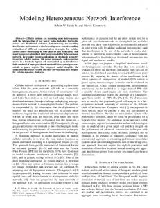
4 Fluid Models for Worms and Failures 4.1 Worms Computer “worms" are programs that self-propagate across a network exploiting security or policy flaws in widely-used services. In recent years, two major classes of worms, scan-based worms and email worms, have frequently attacked the Internet. Email worms propagate through emails and compromise computers when email users execute worm email attachments or simply view worm emails --- they require human interference to propagate and thus propagate relatively slowly. On the other hand, scan-based worms propagate by generating IP addresses to scan and directly compromise any vulnerable target computer --- they need no human activation and thus are able to propagate much faster than email worms. For example, Slammer in January 2003 infected more than 90% of vulnerable computers in the Internet within just 10 minutes. Recent well-known worms, Code Red, Code Red II, Slammer, Blaster, Sasser, are all scan-based worms. We concentrate on scan-based worms.

9

Attackers have tried many scanning strategies in previous worms. Code Red and Slammer uniformly scanned the entire IPv4 space. Code Red II used a local preference scan: it had a higher probability to scan an address within the same Class B or Class A network than a random address. Blaster sequentially scanned the Internet and chose its sequential-scan starting point from a local address with probability 0.4. Based on classical epidemic spreading models, we have developed fluid models that can be used to study different scanning strategies such as those mentioned above. We present a simple model for a worm using a simple random scanning policy and then describe how it can be adapted to model other policies. Consider a population of N vulnerable hosts, each of which has its own IP address. Let I(t) denote the number of infectious hosts at time t. Then [N- I(t)] is the number of susceptible hosts at time t. The epidemic model for a homogeneous system is: dI(t)/dt = β I(t)[N-I(t)] where β is the pairwise rate of infection in epidemiology studies from infectious hosts I(t) to susceptible hosts [N- I(t)]. At t = 0, I(0) hosts are infectious and the other [N-I(0)] hosts are all susceptible. Now β is given in terms of the scan rate of a computer, η, and the size of the address space, Ω, within which lie the vulnerable hosts. For example, in the case of Code Red, N=360,000, η=358 scans /min., and Ω=232. Figure 5 shows how the number of infected hosts grows as a function of time. One observes that Code Red requires several hundred minutes to take off. 400000 350000

No. infected

300000 250000 200000 150000 100000 50000 0 0

100

200

300

400

500

600

Time (minutes) Figure 5: The classic Code Red worm

The model can be used to evaluate the performance of a number of different scanning strategies. These include:

10

•

Idealized worm: All infected nodes are perfectly synchronized scanning only vulnerable hosts and only once.

•

Flash worm: Infected worms know the identities of all vulnerable hosts and perform a random scan over them.

In both cases Ω = Ν. The performances of such worms are illustrated in Figure 6 with and without a two second infection delay. 4.E+05

No. infected

4.E+05 3.E+05

perfect worm with delay flash worm with delay

3.E+05 2.E+05 2.E+05 1.E+05 5.E+04 0.E+00

0

2

4 6 8 10 12 14 Time (seconds)

Figure 6: Idealized and flash worms with and without a two second delay

We have also adapted the model to study routing and local preference worms. Briefly, a routing worm is one that uses BGP routing tables to avoid portions of the IP address space that do not contain hosts. This has the effect of reducing the search space by 70%. A local preference worm scans addresses in the vicinity of the infected host with higher probability than distant addresses. Additional details of the models and its analysis are found in [8]. Figure 7 illustrates the performance of a routing worm and a local preference worm where the host scans addresses in its vicinity with probability 0.5. From our analysis, we derive the following understanding of worm scanning strategies: •

Cooperation among infected hosts for scanning does not significantly increase a worm's spreading speed.

•

A local preference scan increases a worm's propagation speed when vulnerable hosts are not uniformly distributed. The optimal local-scan probability increases as a function of the localscan network size.

•

When vulnerable hosts are uniformly distributed, divide-and-conquer scan, sequential scan, and uniform scan are equivalent in terms of a worm's propagation speed.

11

•

A flash worm that uses uniform scan is an optimal spreading worm converged both from hitlist worm and from routing worm; a flash worm that makes sure no IP address is scanned more than once is the fastest spreading worm in terms of worm scanning strategy.

•

For a sequential scan worm, such as Blaster, using local preference in selecting its starting point slows down the worm's propagation speed.

•

For a selective attack worm, such as a routing worm [8], when the density of vulnerable hosts in the target domain is higher than the density in other domains, the worm propagates faster in the target domain if it only scans the target domain instead of all domains (and vice versa).

No. infected

400000 350000 300000 250000 200000 150000 100000 50000

Uniform worm Routing worm Local preference worm

0 0

100 200

300 400 500 600

Time (minutes) Figure 7: Comparison of routing and local preference worms with Code Red

In addition, based on our models, we have developed statistical detection algorithms for worms. Briefly, they look for an exponential increase in scan traffic that is characteristic of the spread of a worm. Additional details are found in [9], as well as in Appendix C of this report.

4.2

Cascading BGP failures

The Internet is a large collection of Autonomous Systems (AS) connected by the BGP routing infrastructure. The BGP maintains connectivity between AS’s. It automatically reconfigures and computes routing tables when it detects a link failure. This computation starts locally around the failure point, and the information propagates through the Internet. The Internet routing table convergence has been observed to take tens of minutes. We developed models that reflect the behavior of BGP. Our analysis confirms that it is indeed possible to have cascading failures in the BGP routing infrastructure. Our results indicate the presence of phase transitions in these systems, and the presence and intensity of the phase transitions are strongly dependent on system parameters. We use the term phase transitions in the sense used by Erdös and Renyi in their work on random graphs that is “an abrupt change in a global system property”. The phase transition is to be interpreted as a sharp threshold rather than the definition used in statistical 12

mechanics. In our analysis, we observe that the propensity for phase transitions increases as clique size increases, and additionally also increases as the processing capacity of the routers decreases. We consider a simple scenario with a finite set of N routers that are all connected to each other, i.e., form a clique. Let the number of down routers at any instant be D(t). We define a “down” router to be one that does not have a functioning routing table, so a router that is in the process of rebooting and obtaining state dumps is also defined to be “down”. Now, we study the system of the number of down routers. The arrival and departure process to the system is defined as:

α(t) := number of arrivals in [0; t) δ(t) := number of departures in [0; t) Consider the process δ(t). The down routers come up with the help of the routers that are currently up (N(t)- D(t)). We define the service rate of an up router as ks, where ks is the average number of down routers a functioning router restores per unit time. Now, if N(t)-D(t) servers are up and providing service, the service received by a single down node is its share of the total service capacity of the system. Thus, the share received by a single router is (N(t) -D(t))/D(t). To account for the boundary condition D = 0, the denominator should actually be the term (D(t) + ka), where ka represents the ambient load on the servers, representing, for instance, processing of normal route advertisements, and prevents D → - ∞. However, for simplicity of exposition, we ignore the term as it does not affect the main observation we obtain later. Hence, the number of departures in an infinitesimal time dt, d±(t), is defined by dδ (t) = D(t) (N(t) - D(t))/D(t) ksdt = (N(t) - D(t)) ksdt

(10)

Resetting BGP sessions leads to two kinds of messages, withdrawal announcements and subsequently full state updates when the BGP session is restored. We model the rate at which a functioning router goes down due to the load imposed by the resetting of a single BGP session as kl. Typically, we expect ks >> kl, as BGP resets are not uncommon and restoring a single session is unlikely to cause a peer router to go down. Now, the average arrivals in an infinitesimal time dt, dα(t), is given by the product of three quantities: the constant kl, the number of routers (BGP sessions) that are currently down D(t) (denoting the total load offered), and finally the number of routers currently up (that can go down), (N(t) - D(t)), i.e., dα (t) = klD(t)(N(t) - D(t))dt

(11)

Now D(t) is α (t - δt), hence combining (9) and (10) yields after some manipulation the following relation dD/dt = - klD2 + (ks + kl N)D – ksN This is a Riccati equation, and without going into the actual solution of the equation, we immediately observe that the dynamical system described by this model exhibits a phase transition: If the initial stateD(0) of the system is above a certain threshold, then as limt→∞ D(t) = N, else lim t→∞ D(t) = 0. In other words, if by some exogenous process (e.g. CODE RED) we

13

manage to bring a certain number of the routers down, thereby resetting the BGP sessions, then depending upon that number, the system either fully recovers or there is a cascading failure. A simulation of the system with different initial conditions is shown in Figure 8, where ks /kl = 20 and we plot two trajectories, one with D(0) = 21 and another with D(0) = 19. Additional details of this work can be found in [10], as well as in Appendix D of this report.

Figure 8: Illustration of how the initial number of failed routers can result in very different behavior

5 Congestion Controllers In Section 3, we presented a model that describes the behavior of a set of TCP flows in a network of AQM-based routers. Their behavior is described by a set of differential equations, which is the language of control theory. For example, the behavior of a single TCP flow traversing a single bottleneck queue is illustrated in Figure 9. congested queue

C

1

1 R tt

W& _ _

W

∫

1 R tt

1 2

⊗ Time Delay

Rtt

N

_ _

q&

∫

TCP load factor 1 R tt

⊗

p

Control law (e.g. RED)

TCP window control Figure 9: Control theoretic diagram of TCP

14

q

In the initial stages of the project, we performed a control theoretic analysis of the RED AQM protocol and presented guidelines for how to set its parameters. In the process of doing this, we uncovered a number of deficiencies of RED and proposed instead a new AQM algorithm based on proportional integral control. Two problems exhibited by RED are as follows: •

the queue averaging mechanism introduces additional delay in the TCP control loop which makes TCP unstable in many situations.

•

RED couples the loss exhibited by a TCP session with the delay that its packets incur.

The new PI AQM controller introduces phase lead, which is ideal for systems with feedback delay. This leads to a speed of response faster than that of a stable RED mechanism. In addition, it decouples loss and delay; in particular, it is possible to specify a fixed queuing delay with a PI controller. Figure 10 compares the performance of a set of TCP sessions under RED and PI.

Figure 10: RED vs. PI control

Details of this work can be found in [11] which is found in the Appendix. As part of the project, we also studied the problem of providing differential Quality of Service (QoS) to classes of TCP sessions. Specifically, we develop algorithms based on the IETF proposed DiffServ architecture [12], [13] to provide minimum throughput guarantees to different collections of TCP sessions. These algorithms rely on two components, multi-level PI AQM controllers residing at core routers that drop or mark packets differentially according to their colors and PI rate controllers residing at edge routers that monitor the throughput of these collections of TCP flows, marking packets as either red or green depending on whether or not the aggregate throughput exceeds its minimum rate. Details are found in [14], which is found in Appendix E. Other results from this project include a study of the effect of uncontrollable flows on the behavior of TCP [15] and the development of algorithms to automatically tune AQM policies such as RED and PI [16].

15

6 Tools As part of our project, we have implemented our fluid modeling methodology into the ns simulation software package. In particular, we developed a fluid network node that accepts packets as inputs, converts them into fluids, and then outputs packets after suffering appropriate losses and delays as predicted by the fluid model. This is illustrated in Figure 11. Additional details can be found in [17], as well as in Appendix F.

Figure 11: Fluid simulation module within ns

7 Summary Our project significantly advanced the state-of-the-art in scalable modeling and simulation. We were the first to introduce the use of fluid models for the characterization of TCP flows within a large network. This is not standard practice. We were the first to begin to examine TCP behavior, coupled with AQM, using control theoretic principles. This is now standard practice and has resulted in significant advances in the development of better control mechanisms. Finally, we were the first to use fluid models to characterize worm spreading and cascading failures within the Internet. Again, this has become standard practice. Finally, references [18] – [43] include additional results related to what has been discussed so far in the report. They are not included in the Appendix.

8 Acknowledgments We would like to acknowledge a number of individuals who made contributions to the work reported here. These individuals are Tian Bu, Yossi Chait, Yu Gu, Jim Kurose, Francesco LoPresti, Yujing Wu, Honggang Zhang, Cliff Zou. We also would like to acknowledge Greg Hadynski for his help in preparing this final report.

16

9 References 9.1

Main Report

1. S. McCanne, S. Floyd. “ns-LBL Network Simulator.” 2. S. Floyd, V. Jacobson. “Random early detection gateways for congestion avoidance,” IEEE/ACM Trans. on Networking, 1(4), Aug. 1997. 3. V. Misra, W. Gong, D. Towsley. “A Fluid-based Analysis of a Network of AQM Routers Supporting TCP Flows with an Application to RED,” Proceedings ACM SIGCOMM'00 September 2000. 4. Y. Liu, F. Lo Presti, V. Misra, D. Towsley, Y. Gu. “Scalable Fluid Models and Simulations for Large-Scale IP Networks,” ACM Transactions on Modeling and Computer Simulation, 14(3), 305-324, July 2004. 5. J. Padhye, V. Firoiu, D. Towsley, J. Kurose. “Modeling TCP Throughput: A Simple Model and its Empirical Validation,” Proc. ACM SIGCOMM'98, (Vancouver, CA, Sept. 1998). To appear in IEEE/ACM Transactions on Networking. 6. T Bu, D. Towsley. “Fixed Point Approximations for TCP Behavior in an AQM Network,” Proceedings of ACM SIGMETRICS 2001, June 2001. 7. S. Sahu, P. Nain, D. Towsley, C. Diot, V. Firoiu. “On Achievable Service Differentiation with Token Bucket Marking for TCP,” Proceedings ACM SIGMETRICS'00, June 2000. 8. Cliff C. Zou, Don Towsley, Weibo Gong. “On the Performance of Internet Worm Scanning Strategies,” UMass ECE Technical Report TR-03-CSE-07, November, 2003. 9. C.C. Zou, W. Gong, D. Towsley, L. Gao. “The monitoring and early detection of Internet worms,” to appear in IEEE/ACM Transactions on Networking. 10. E.G. Coffman Jr., Z. Ge, V. Misra, D. Towsley. “Network Resilience: Exploring Cascading Failures within BGP,” Proceedings of the 40th annual Allerton Conference on Communications, Computing and Control, October 2002. 11. C. Hollot, V. Misra, D. Towsley, W. Gong. “Analysis and Design of Controllers for AQM Routers Supporting TCP Flows,” IEEE Transactions on Automatic Control, 47(6), 945-959, June, 2002. 12. J. Heinanen, F. Baker, W. Weiss, J. Wroclawski. “Assured forwarding PHB group,” RFC 2597, June 1999. 13. J. Heinanen, R. Guerin. “A two rate three color marker,” RFC 2698, Sept. 1999. 14. Y. Chait, C.V. Hollot, V. Misra, D. Towsley, H. Zhang, Y. Cui. “Throughput Differentiation Using Coloring at the Network Edge and Preferential Marking at the Core,” to appear in IEEE/ACM Transactions on Networking. 15. C. V. Hollot, Yong Liu, Vishal Misra, Don Towsley. “Unresponsive Flows and AQM Performance,” Proc. INFOCOM 2003. 16. H. Zhang, C.V. Hollot, D. Towsley, V. Misra. “A Self-Tuning Structure for Adaptation in TCP/AQM Networks,” Proceedings of Globecom 2003. 17. Y. Gu, Y. Liu, D. Towsley. “On Integrating Fluid Models with Packet Simulation,” Proceedings of INFOCOM 2004, March 2004. 18. C.V. Hollot, V. Misra, D. Towsley, W. Gong. “A Control Theoretic Analysis of RED,” Proc. INFOCOM 2001, April 2001. 19. C.V. Hollot, V. Misra, D. Towsley, W. Gong. “On designing improved controllers for AQM routers supporting TCP flows,” Proc. INFOCOM 2001, April 2001.

17

20. E. Graves, R. Srikant, D. Towsley. “Decentralized Computation of Weighted Max-Min Fair Bandwidth Allocation in Networks with Multicast Flows,” Proc. of the 2001 International Workshop on Digital Communications 2001- Evolutionary Trends of the Internet, Taormina, Italy, Sept 17-20, 2001 21. W. Gong, Y. Liu, V. Misra, D. Towsley “On the web file size distributions,” Proc. 2001 Allerton Conference, Oct. 2001. 22. C.V. Hollot, Y. Chait. “Nonlinear Stability Analysis for a Class of TCP/AQM Networks,” Proc. 40th IEEE CDC, Dec. 2001. 23. Y. Liu, W. Gong. “On fluid queueing system with strict priority,” Proc. of 40th IEEE CDC, Dec. 2001. 24. Y. Liu, W. Gong, P. Shenoy. "The Impact of Concurrent Downloads", Proc. of Winter Simulation Conference 2001, Dec. 2001. 25. Y. Chait, C.V. Hollot and Vishal Misra, “Analysis of TCP Networks with AQM,” Proceedings of the 2002 American Control Conference, Anchorage, (2430-2435), 2002. 26. Y. Chait, C.V. Hollot, V. Misra, D. Towsley, H. Zhang and C.S. Lui, “Providing Throughput Differentiation for TCP Flows using Adaptive Two-Color Marking and Multi-Level AQM,” Proceedings of the 2002 IEEE Infocom, New York, 2002. 27. T. Bu, D. Towsley. “On Distinguishing between Internet Power Law Topology Generators,” Proc. INFOCOM 2002, New York, 2002. 28. W. Wei, B. Wang, D. Towsley. “Continuous-time Hidden Markov Models for Network Performance Evaluation”, Performance Evaluation 49, 129-146, September 2002. 29. D. R. Figueiredo, B. Liu, V. Misra, D. Towsley "On the Autocorrelation Structure of TCP Traffic" Computer Networks Journal Special Issue on "Advances in Modeling and Engineering of Long-Range Dependent Traffic", 2002. 30. W. Gong, D. Towsley, Y. Wu and D. Ye. “A Stochastic Differential Equation Model for Queues with Traffic Smoothing”, Proc. 2002 Allerton Conference on Communications, Control, and Computing, 3 October, 2002. 31. C.V. Hollot and Y. Chait, "The Dynamic of Pricing in a TCP/AQM network," Proc. 2002 Allerton Conference on Communications, Control, and Computing, 3 October, 2002. 32. C. Zhou, W. Gong, D. Towsley. “Code Red Worm Propagation Modeling and Analysis”, in Proc. 2002 ACM Conf. on Computer and Communications Security, Oct. 2002. 33. J. Xiong, W. Gong. “A novel algorithm for network reliability analysis”, Proceedings of International Conference on Telecommunications, Nov. 18, 2002. 34. Y. Liu, W. Gong. “Challenges to Congestion Control Posed by Concurrent Downloads,” Proc. CDC2002, December 2002. 35. Y. Liu, F. Lo Presti, V. Misra, D. Towsley, Y. Gu. "Fluid Models and Solutions for LargeScale IP Networks", Proc. Sigmetrics 2003, June 2003. 36. Y. Wu, W. Gong. ``Accuracy Study of Time-Stepped Simulation of High Speed Networks,'' Proc. IEEE International Conference on Communications (ICC 2003), May 2003. 37. J. Xiong, W. Gong, C. Qiao, "An Effective Method for Blocking Performance Analysis of WDM All-Optical Networks", Journal of Lightwave Technology pp.1421-1434, June 2003. 38. Y. Wu, W. Gong, "Burst Level Simulation of a Queueing System with Active-Idle Sources", IEEE Pacific Rim Conference on Communications, Computers, and Signal Processing, Victoria Canada, August 2003. 39. C.C. Zou, W. Gong, D. Towsley, “Worm Propagation Modeling and Analysis under Dynamic Quarantine Defense,” Proc. of Workshop on Rapid Malcode, Oct. 2003.

18

40. Y. Liu, W. Gong, ``On Fluid Queueing System with Strict Priority'' IEEE Transactions on Automatic Control, December 2003. 41. Y. Wu, W. Gong, D. Towsley. "Analysis of Abstract Simulation Via Stochastic Differential Equation Models", Proceedings of IEEE Conference on Decision and Control 2003, Hawaii, December 2003. 42. X. Yu, C. Qiao, Y. Liu, “TCP Implementations and False Time Out Detection in Optical Burst Switching Networks,” INFOCOM 2004, March 2004. 43. W. Gong, Y. Liu, V. Misra, D. Towsley. "Self-Similarity and Long Range Dependence on the Internet: A second look at the evidence, origins and implications'', to appear in Computer Network Journal. 44. Y. Liu, Y. Gu, H. Zhang, W. Gong and D. Towsley. "Application Level Relay for Highbandwidth Data Transport'', to appear in the First Workshop on Networks for Grid Applications (GridNets), San Jose, October 2004. 45. Cliff C. Zou, Don Towsley, and Weibo Gong. "Email Worm Modeling and Defense". To appear in 13th International Conference on Computer Communications and Networks (ICCCN'04), October 2004 (Best Paper Nominee). 46. H. Han, S. Shakkottai, C.V. Hollot, R. Srikant, D. Towsley. ”Overlay TCP for Multi-Path Routing and Congestion Control”, to appear IEEE/ACM Trans. On Networking. 9.2

Appendix A

1. K. J. Astrom and B. Wittenmark. Computer Controlled Systems: Theory and Design. Prentice-Hall, 1984. 2. R. Brockett. Stochastic control. Lecture Notes, Harvard University. 3. D. D. Clark and W. Fang. Explicit allocation of best effort packet delivery service. ACM Transations on Networking, August 1998. 4. W. Feng, D. Kandlur, D. Saha, and K. Shin. Blue: A New Class of Active Queue Management Algorithms. Technical report, UM CSE-TR-387-99, 1999. 5. W. Feng, D. D. Kandlur, D. Saha, and K. G. Shin. A Self-Configuring RED Gateway. In Proceedings lnfocom 1999. V. Firoiu and M. Borden. A study of active queue management for congestion control. In Proceedings Infocom 2000. 6. S. Floyd. Recommendation on using the "gentle" variant of RED. http://www.aciri.org/floyd/red/gentle.html, March 2000. 7. S. Floyd and V. Jacobson. Random Early Detection gateways for congestion avoidance. IEEE/ACM Transactions on Networking, 1(4), August 1997. 8. I. Matta and A. U. Shankar. Z-iteration: Efficient estimation of instantaneous measures in time-dependent multi-class systems. In Proceedings SIGMETRICS/Performance '95. 1995. 9. M. May, T. Bonald, and J.-C. Bolot. Analytic Evaluation of RED Performance. Proc. lnfocom 2000. 10. V. Misra, W. B. Gong, and D. Towsley. Stochastic Differential Equation Modeling and Analysis of TCP Window size Behavior. Technical Report ECE-TR-CCS-99-10-01, 1999. Presented at Performance 99, October 1999 Istanbul. Available at ftp://gaia.cs.umass.edu/pub/Misra99-TCP-Stochastic.ps.gz. 11. T. J. Ott, T. V. Lakshman, and L. H. Wong. SRED: Stabilized RED. Proc. lnfocom 1999. 12. J. Padhye, V. Firoiu, D. Towsley, and J. Kurose. Modeling TCP throughput: A simple model and its empirical validation. In Proceedings of ACM/SIGCOMM, 1998.

19

13. M. Vojnovic, J. Y. Le Boudec, and C. Boutremans. Global fairness of additive-increase and multiplicative-decrease with heterogeneous round-trip times. Proc. INFOCOM 2000, March 2000.

9.3

Appendix B

1. F. Baccelli, D. McDonald, J. Reynier. A Mean-field Model for Multiple TCP Connections through a Buffer. In Proceedings of lFIP WG 7.3 Performance’02, Sept. 2002. 2. S. Floyd, V. Jacobson. Random Early Detection gateways for congestion avoidance. IEEE/ACM Transactions on Networking 1, 4, 397-413, Aug. 1993. 3. C. Hollot, V. Misra, D. Towsley, W. Gong. On designing improved controllers for AQM routers supporting TCP flows. In Proceedings of INFOCOM 2001, 2001. 4. S. Kunniyur, R. Srikant. Analysis and design of an adaptive virtual queue algorithm for active queue management. In Proceedings of ACM/SIGCOMM '2001, Aug. 2001. 5. K. Psounis, R. Pan, B. Prabhakar, D. Wischik. The scaling hypothesis: simplifying the prediction of network performance using scaled-down simulations. ACM Computer Communications Review, 2003. 6. P. Tinnakornsrisuphap, A. Makowski. Limit Behavior of ECN/RED Gateways Under a Large Number of TCP Flows. In Proceedings Infocom 2003, 2003.

9.4

Appendix C

1. Symantec Corp.: Symantec early warning solutions. http://enterprisesecurity.symantec.com/SecurityServices /content.cfm?ArticleID=1522. 2. eEye digital security: .ida "Code Red" worm. http://www.eeye.com/html/Research/Advisories/AL20010717.html, 2001. 3. eEye digital security: Blaster worm analysis. http://www.eeye.com/html/Research/Advisories/AL20030811.html, 2003. 4. B.D.O. Anderson and J. Moore. Optimal Filtering. Prentice Hall, 1979. 5. D. Anderson, T. Frivold, and A. Valdes. Next-generation intrusion detection expert system (nides) a summary. Technical Report SRI-CSL-95-07, SRI International, May 1995. 6. V. H. Berk, R.S. Gray, and G. Bakos. Using sensor networks and data fusion for early detection of active worms. In Proceedings of the SPIE AeroSense, 2003. 7. Cooperative association for Internet data analysis. http://www. caida.org. 8. CERT Coordination Center. http://www.cert.org. CERT. CERT/CC advisories. http://www.cert.org/advisories/. 9. Z. Chen, L. Gao, and K. Kwiat. Modeling the spread of active worms. Proc. INFOCOM, March 2003. 10. D. Dagon, X. Qin, G. Gu, W. Lee, J. Grizzard, J. Levin, and H. Owen. Honeystat: Local worm detection using honeypots. In Proceedings of the 7th International Symposium on Recent Advances in Intrusion Detection (RAID), September 2004. 11. D.J. Daley and J. Gani. Epidemic Modeling: An Introduction. Cambridge University Press, 1999. 12. D. Denning. An intrusion detection model. IEEE Transactions on Software Engineering, 13(2), 1987.

20

13. D. Goldsmith. Incidents maillist: Possible CodeRed connection attempts. http://lists.jammed.com/incidents/2001/07/0149.html. 14. S. A. Hofmeyr, S. Forrest, and A. Somayaji. Intrusion detection using sequences of system calls. Journal of Computer Security, 6(3), 1998. 15. Honeynet project. Know your enemy: Honeynets.http://project.honeynet.org/papers/honeynet. 16. Internet Storm Center. http://isc.incidents.org. 17. J. Jung, V. Paxson, A. W. Berger, and H. Balakrishnan. Fast portscan detection using sequential hypothesis testing. In Proceedings of the IEEE Symposium on Security and Privacy, May 2004. 18. J. Jung, S. E. Schechter, and A. W. Berger. Fast detection of scanning worm infections. In Proceedings of the 7th International Symposium on Recent Advances in Intrusion Detection (RAID), September 2004. 19. J.O. Kephart, D. M. Chess, and S.R. White. Computers and epidemiology. IEEE Spectrum, 30(5), May 1993. 20. J.O. Kephart and S.R. White. Directed-graph epidemiological models of computer viruses. In Proceedings of IEEE Symposium on Security and Privacy, pages 343-359, 1991. 21. J.O. Kephart and S.R. White. Measuring and modeling computer virus prevalence. In Proceedings of IEEE Symposium on Security and Privacy, 1993. 22. H. Kim and B. Karp. Autograph: Toward automated, distributed worm signature detection. In Proceedings of 13th USENIX Security Symposium, August 2004. 23. W. Lee and S. Stolfo. A framework for constructing features and models for intrusion detection systems. ACM Transactions on Information and System Security, 3(4), 2000. 24. L. Ljung and T. Soderstrom. Theory and Practice of Recursive Identification. MIT Press, 1983. 25. D. Moore, V. Paxson, S. Savage, C. Shannon, S. Staniford, and N. Weaver. Inside the Slammer worm. IEEE Magazine on Security and Privacy, 1(4), July 2003. 26. D. Moore, C. Shannon, and J. Brown. Code-Red: a case study on the spread and victims of an Internet worm. In Proceedings of the second ACM SIGCOMM Workshop on Internet Measurement, November 2002. 27. D. Moore, C. Shannon, G. M. Voelker, and S. Savage. Internet quarantine: Requirements for containing self-propagating code. Proc. INFOCOM, March 2003. 28. D. Moore, C. Shannon, G.M. Voelker, and S. Savage. Network telescopes: Technical report. Technical Report TR-2004-04, CAIDA, 2004. 29. R. Pang, V. Yegneswaran, P. Barford, V. Paxson, and L. Peterson. Characteristics of Internet background radiation. In Proceedings of the Internet Measurement Conference (IMC), October 2004. 30. N. Provos. A virtual honeypot framework. In Proceedings of 13th USENIX Security Symposium, August 2004. 31. SANS institute. http://www.sans.org. 32. D. Seeley. A tour of the worm. In Proceedings of the Winter USENIX Conference, January 1989. 33. C. Shannon and D. Moore. The spread of the Witty worm. http://www.caida.org/analysis/security/witty/, March 2004. 34. S. Singh, C. Estan, G. Varghese, and S. Savage. Automated worm fingerprinting. In Proceedings of the 6th ACM/USENIX Symposium on Operating System Design and Implementation (OSDI), December 2004.

21

35. S. Staniford. Containment of scanning worms in enterprise networks. Journal of Computer Security, 2003. 36. S. Staniford, V. Paxson, and N.Weaver. How to own the Internet in your spare time. In Proceedings of USENIX Security Symposium, August 2002. 37. S. Staniford-Chen, S. Cheung, R. Crawford, M. Dilger, J. Frank, J. Hoagland, K. Levitt, C. Wee, R. Yip, and D. Zerkle. GrIDS a graph-based intrusion detection system for large networks. In Proceedings of the 19th National Information Systems Security Conference, October 1996. 38. A. Valdes and K. Skinner. Adaptive, model-based monitoring for cyber attack detection. In Proceedings of the 3th International Symposium on Recent Advances in Intrusion Detection (RAID), October 2000. 39. D. Verton. DHS launches cybersecurity monitoring project. http://www.pcworld.com/news/article/0, aid, 1 12764,00. asp, October 2003. 40. N. Weaver, S. Staniford, and V. Paxson. Very fast containment of scanning worms. In Proceedings of 13th USENIX Security Symposium, August 2004. 41. M. M. Williamson. Throttling viruses: Restricting propagation to defeat mobile malicious code. In 18th Annual Computer Security Applications Conference, December 2002. 42. J. Wu, S. Vangala, L. Gao, and K. Kwiat. An efficient architecture and algorithm for detecting worms with various scan techniques. In Proceedings of the 11th Annual Network and Distributed System Security Symposium (NDSS'04), February 2004. 43. C. C. Zou. Internet worm propagation simulator. http://tennis.ecs.umass.edu/~czou/research/wormSimulation.html, February 2004. 44. C. C. Zou, L. Gao, W. Gong, and D. Towsley. Monitoring and early warning for Internet worms. In Proceedings of 1 0th ACM Conference on Computer and Communications Security (CCS'03), October 2003. 45. C. C. Zou, W. Gong, and D. Towsley. Code Red worm propagation modeling and analysis. In Proceedings of 9th ACM Conference on Computer and Communications Security (CCS'02), October 2002. 46. C. C. Zou, W. Gong, and D. Towsley. Worm propagation modeling and analysis under dynamic quarantine defense. In Proceedings of ACM CCS Workshop on Rapid Malcode (WORM'03), October 2003. 47. C. C. Zou, D. Towsley, and W. Gong. On the performance of Internet worm scanning strategies. Technical Report TR-03-CSE-07, Umass ECE Dept., November 2003. 48. C. C. Zou, D. Towsley, and W. Gong. Email worm modeling and defense. In Proceedings of 13th International Conference on Computer Communications and Networks (ICCCN'04), October 2004. 49. C. C. Zou, D. Towsley, W. Gong, and S. Cai. Routing worm: A fast, selective attack worm based on IP address information. Technical Report TR-03-CSE-06, Umass ECE Dept., November 2003. 9.5 1.

Appendix D

J . C o w i e , A . O g i e l s k i , B . P r e m o r e , a n d Y . Y u a n , " G l o b a l R o u t ing Instabilities during Code Red II and Nimda Worm Propagation," http://www.renesys.com/projects/bgpinstability, September 2001.

22

2. 3. 4. 5. 6. 7. 8.

9. 10.

11.

9.6

B. R. Hurley, C. J. R. Seidl, and W. F. Sewell, "A Survey of Dynamic Routing Methods for Circuit-Switched Traffic," IEEE Communications Magazine, vol. 25, no. 9, September 1991. K. Varadhan, R. Govindan, and D. Estrin, "Persistent route oscillations in inter-domain routing," Computer Networks, vol. 32, no. 1, pp. 1-16, Jan. 2000. C. Labovitz, A. Ahuja, A. Abose, and F. Jahanian, "An experimental study of delayed internet routing convergence," Proceedings ACM SIGCOMM, Aug. 2000. C. Labovitz, A. Ahuja, R. Wattenhofer, and S. Venkatachary, "The impact of internet policy and topology on delayed routing convergence," Proc. INFOCOM, 2001, Apr. 2001. Z. M. Mao, R. Govindan, G. Varghese, and R. Katz, "Route Flap Damping Exacerbates Internet Routing Convergence," in Proceedings ACM SIGCOMM, 2002. A. Shaikh, L. Kalampoukas, R. Dube, and A. Varma, "Routing stability in congested networks: Experimentation and analysis," in Proceedings ACM SIGCOMM, 2000. T. Griffin and G. T. Wilfong, "An analysis of BGP convergence properties," in Proc. ACM SIGCOMM, 1999, pp. 277-288. L.Gao and J. Rexford, "Stable internet routing without global coordination," in Proceedings ACM SIGMETRICS, 2000, pp. 307-317. L. Gao, T. Griffin, and J. Rexford, "On Inferring Automonous System Relationships in the Internet," in Proceedings INFOCOM, 2001. L. Wang, X. Zhao, D. Pei, R. Bush, D. Massey, A. Mankin, S. F. Wu, and L. Zhang, "Observation and Analysis of BGP Behavior under Stress," in Internet Measurement Workshop, 2002. D. Daley and J. Gani, Epidemic Modeling. Cambridge University Press, 1999.

Appendix E

1. D.E. Comer, Internetworking with TCP/IP, Principles, Protocols and Architectures, Vol. 1, 4th Edition, Prentice Hall, 2000. 2. S. Floyd and V Jacobson, "Random Early Detection Gateways for Congestion Avoidance," IEEE/ACM Transactions on Networking, Vol. 1, August 1997. 3. K.K. Ramakrishnan, S. Floyd. "A Proposal to Add Explicit Congestion Notification (ECN) to IP," RFC 2481, Jan. 1999. 4. M. Christiansen, K. Jeffay, D. Ott, and F. Smith, "Tuning Red for Web Traffic," Proceedings of ACM SIGCOMM, 2000. 5. M. May, T. Bonald, and J.-C. Bolot, "Analytic Evaluation of RED Performance," Proceedings INFOCOM, 2000. 6. D. Lin and R. Morris, "Dynamics of Random Early Detection," Proceedings ACM SIGCOMM, 1997. 7. M. May, C. Diot, B. Lyles, and J. Bolot, "Influence of Active Queue Management Parameters on Aggregate Traffic Performance," available at ftp://ftp.sprintlabs.com/diot/aqm.zip. 8. T J. Ott, T V Lakshman, and L. H. Wong, "SRED: Stabilized RED," Proceedings INFOCOM, 1999. 9. W Feng, D. Kandlur, D. Saha, and K. Shin, "Blue: A New Class of Active Queue Management Algorithms," tech. rep., UM CSE-TR-387-99, 1999. 10. W Feng, D. D. Kandlur, D. Saha, and K. G. Shin, "A Self-Configuring RED Gateway," Proceedings INFOCOM, 1999. 11. V. Firoiu and M. Borden, "A Study of Active Queue Management for Congestion Control," Proceedings INFOCOM, 2000.

23

12. Y. Zhao, S.Q. Li and S. Sigarto, "A Linear Dynamic Model for Design of Stable Explicit-Rate ABR Control Schemes," Proceedings INFOCOM, 1997. 13. B. Ataslar, P. Quet, A. Iftar, H. Ozbay, T. Kangand S. Kalyanaraman, "Robust Rate-Based Flow Control for High-Speed Networks: The Case of Uncertain Time-Varying Multiple Time Delays," Proceedings of the American Control Conference, Chicago, pp. 2804-2808, 2000. 14. E. Altman T Basar and R. Srikant, "Robust Rate Control for ABR Sources," Proceedings INFOCOM, 1998. 15. S. Mascolo, "Congestion Control in High-Speed Communication Networks," Automatica, Vol. 35, no. 12, pp. 1921-1935, 1999. 16. F. Kelly, "Mathematical Modeling of the Internet," Mathematics Unlimited - 2001 and Beyond, 2000. 17. V. Misra, W B. Gong, and D. Towsley, "Fluid-based Analysis of a Network of AQM Routers Supporting TCP Flows with an Application to RED," Proceedings ACM SIGCOMM, 2000. 18. S. Athuraliya, V H. Li, S. H. Low and Q. Yin "REM: Active Queue Management," IEEE Network, Vol. 15, pp. 48-53, 2001. 19. C. V. Hollot, V. Misra, D. Towsley, and W. B. Gong, "A Control Theoretic Analysis of RED." Proceedings INFOCOM, 2001. 20. C. V Hollot, V Misra, D. Towsley, and W. B. Gong, "On Designing Improved Controllers for AQM Routers Supporting TCP Flows." Proc. INFOCOM, 2001. 21. S. H. Low, F. Paganini, and J.C. Doyle, "Internet Congestion Control," IEEE Control Systems Magazine, Vol. 22, no. 1, pp. 28-43, 2002. 22. G. F. Franklin, J. D. Powell, and A. Emami-Naeini, Feedback Control of Dynamic Systems. Addison-Wesley, 1995. 23. K. J. Astrom, "Oscillations in Systems with Relay Feedback," in Adaptive control, filtering and signal processing, IMA Volume in Mathematics and its Applications, Vol. 74, pp. 1-25, 1995. 24. A. Veras and M. Boda, "The Chaotic Nature of TCP Congestion Control," Proc. INFOCOM, 2000.

9.7

Appendix F

1. "The Network Simulator - ns-2," http://www.isi.edu/nsnam/ns/. 2. "GloMoSim - Global Mobile Information System Simulation Library,"http://pcl.cs.ucla.edu/projects/glomosim/. 3. "QualNet," http://www.scalable-networks.com. 4. "Parallel and Distributed NS," http://www.cc.gatech.edu/computing/compass/pdns/. 5. V. Misra, W.-B. Gong, and D. Towsley, "Fluid-based Analysis of a Network of AQM Routers Supporting TCP Flows with an Application to RED," in Proceedings of ACM SIGCOMM, 2000. 6. Y. Liu, F. L. Presti, V. Misra, D. Towsley, and Y. Gu, "Fluid models and solutions for large-scale ip networks," in Proceedings of ACM SIGMETRICS '2003, June 2003. 7. D. M. Nicol and G. Yan, "Discrete event fluid modeling of background tcp traffic," Department of Computer Science, Dartmouth College, Tech. Rep., To appear in ACM Transactions on Modeling and Computer Simulation, 2004. 8. S. Bohacek, J. P. Hespanha, J. Lee, and K. Obraczka, "A hybrid systems modeling framework for fast and accurate simulation of data communication networks," in Proceedings of ACM SIGMETRICS '2003.

24

9. B. Melamed, S. Pan, and Y. Wardi, "Hybrid discrete-continuous fluid-flow simulation," in Proceedings oflTCOM 2001, Scalability and Traffic Control in IP Networks, August 2001. 10. G. Riley, R. Fujimoto, M. Ammar, K. Permula, and D. Xu, "Distributed network simulations using the dynamic simulation backplane," in Proceedings of International Conference of Distributed Computing Systems, 2001. 11. T. Yung, J. Martin, M. Takai, and R. Bagrodia, "Integration of fluid-based analytical model with packet-level simulation for analysis of computer networks," 2001. [Online]. Available: citeseer.nj.nec.com/ yung0 1 integration, html 12. C. V. Hollot, V. Misra, D. Towsley, and W.-B. Gong, "On Designing Improved Controllers for AQM Routers Supporting TCP Flows," in Proceedings INFOCOM, April 2001. 13. S. Floyd and V. Jacobson, "Random early detection gateways for congestion avoidance," IEEE/ACM Transactions on Networking, vol. 1, no. 4, pp. 397, 1993. 14. J. Winick and S. Jamin, "Inet-3.0: Internet topology generator," 2002. [Online]. Available: citeseer.nj.nec.com/526211.html

25

Appendix A: Fluid-based Analysis of a Network of AQM Routers Supporting TCP Flows with an Application to RED A1.

INTRODUCTION

Active queue management techniques were proposed in [8], [3] to both alleviate some congestion control problems for IP networks as well as provide some notion of quality of service. Modeling and analysis of such networks is important to understand their dynamics. While traditional discrete event simulations work well in general, even the most efficiently coded simulators suffer from the problem of scaling. We exploit fluid modeling to present a general methodology for the analysis of a network of routers that support active queue management with TCP flows. We use Poisson Counter Driven Stochastic Differential Equations to model the behavior of TCP traffic and derive a set of differential equations that describe the AQM policy and the router queuing process. Next, we develop a numerical scheme for obtaining the transient average behavior of a number of metrics including queue length, round trip time and TCP flow throughput from a set of coupled ordinary differential equations that result from our analysis. Given an AQM policy, we are able to get (expected) transient behavior of networks from our solution. We are able to handle large flows without a significant increase in computational complexity. We illustrate our approach by analyzing RED [8] using the techniques developed in Section 3.1. Our solution technique yields predictions that match well with those obtained through simulation. Our modeling and solution methodology lead to a straightforward discovery of a critical problem with the RED averaging mechanism, one not addressed elsewhere. Our scheme has similar aims, to obtain transient behavior by numerical solution of a system of equations, to a heuristic approach proposed in [9]. It is however not clear how and why the heuristics work in cases reported.

A2.

APPLICATION TO THE RED ACTIVE QUEUE MANAGEMENT POLICY

We now present an application of the system, taking RED as the AQM policy, which has been shown to outperform Drop-Tail queues under certain scenarios. RED is a powerful mechanism to control traffic, potentially solving problems like flow synchronization, correlation of drop events while providing consistently high link utilizations. However, numerous problems have been cited with RED [10]. RED works well in certain scenarios, whereas it does very poorly, even worse than Drop-Tail, in other cases [6]. There is no clear understanding on how to tune various RED parameters that work well in all scenarios. Consequently, there is considerable nervousness in the community regarding deployment of RED, and numerous variations of RED have been proposed [5], [12], [4]. Some of the schemes have self-tuning parameters, while others maintain per-flow state. It is clear that there is a great need for thoroughly understanding the behavior of RED. We believe our techniques can help in that effort. We first consider a system in which there is a single congested router with a transmission capacity of C. Associated with this router is an active queue management (AQM) policy that is characterized by a packet discard function p(x) that takes as its argument an estimate of the average queue length at the router. The queue length of the router is denoted by q(t), t > 0. The

26

classical example of an AQM policy is RED [8] for which p(x) takes the form in the Figure below where tmin, tmax, and pmax are configurable parameters. Figure 12: RED drop function

We will compare the results obtained from our model to those obtained from simulating an equivalent system using the well-known ns simulator. Our differential equation solver was implemented as a MATLAB program (a simple implementation with 42 total lines of code) which takes the matrix A, where the rows represent the different flows and the columns represent the different routers (queues) in a network, and a link capacity vector C as input. We did not incorporate slow-start in our program. All routers are assumed to have the same RED parameters. The propagation (non-queueing) delay for each class of flows is kept at 200 ms. The buffers are sized so that all losses are RED-related, i.e. no drop-tail losses occur on the network. The tmin is 150 packets and the tmax is 200 packets. δ is a parameter in our solver which is not specified in RED. Instead RED updates the queue size estimate on the arrival of each packet. We can account for it in two different ways •

ns updates the queue at every packet arrival. Thus, we choose δv to be l/bv, where bv is the instantaneous arrival rate at a queue measured in packets. δv thus becomes a function of time.

•

We choose a fixed value of Sv. If the queue is stable, then the steady state arrival rate = service rate. Then, for each (bottlenecked) queue, Sv is simply 1/Cv where Cv is the capacity of link v in terms of (average) sized packets per second.

Note that both techniques are approximate. In our implementation we use 1/Cv as an estimate of δ v.

A2.1. Experiment topology We use the simple topology shown in the Figure below. It consists of two RED queues Ql and Q2. Both links have three sets of flows going through them. S2 goes through both the queues, whereas S1, S3 and S4, S5 go through only Q1 and Q2 respectively. The only bottleneck links are the queues Ql and Q2. We'll show results from 5 different experiments performed using ns and our DE solver.

27

Figure 13: Simple network topology

We tabulate the parameter choices in the various experiments in the following table for reference.

A2.2. Experiment 1 We first consider a symmetric case, where both RED queues have similar bandwidth capacity of 5Mb/s. a is kept at 0.0001, pmax = 0.1. Each class of flows consists of 40 individual flows which start at t = 0 (200 flows in all). At time t = 75, three fourths of the flows in each class drop out (so there are only 10 flows in each class). At time t = 150, those flows restart. We plot the Queue estimate and instantaneous queue length for Queue 1 and 2 in plots (a) and (b) of the following Figure respectively along with our model predictions of the expected values for the same. Note that we are plotting the results of one ns simulation along with our solution which gives the expected results. As we can see, the differential equation solution tracks the simulations pretty well, tracking both the average queue estimate and the instantaneous queue length well. Our method adapts to the changing nature of the load as well. Note that our solution differs initially from the simulation in all cases, because we didn't implement the effect of slow start.

28

Figure 14: Symmetric case, plots for Queue 1, Experiment 1

Figure 15: Symmetric case, plots for Queue 2, Experiment 1

A2.3. Experiment 2 Now we repeat the experiment in an asymmetric setting. We reduce the link capacity of the second queue to be 2.5Mb/s from 5Mb/s. Again we show the average queue estimate and instantaneous queue length along with our DE estimates for both the queues in the following Figures and our results match well with ns simulations for both the queues. Notice that the average queue estimate stays higher for Queue 2 which is correctly reflected in our DE solution.

29

Figure 16: Asymmetric case, plots for Queue 1, Experiment 2

Figure 17: Asymmetric case, plots for Queue 2, Experiment 2

If we focus on the middle portion of the Figures above (when only a fourth of the flows are active), we observe that Queue 1 exhibits more oscillations than Queue 2. The oscillations are not good for the network as they may result in unacceptably large queue lengths and hence a large variability in delays for the flows going through. Even if the mean delay may turn out to be the same, these oscillations add considerable jitter to the delays. If the buffer is not large enough, then the effect of the oscillations will be to cause buffer overflows. They also cause periodically high RED loss rates and affect the throughput adversely. The question is: why? The larger bandwidth capacity of Queue 1 certainly plays a part, reducing stability margins, however we would like to point out another, hidden, cause. The queue averaging module is essentially a first order low pass filter. The original design goal of RED was to track the average queue size (low frequency signal), and to filter out bursts (high frequency signal). The input to this filter is the instantaneous queue length, and the output is the average queue estimate. Asymptotically, the frequency response of this filter is described by the magnitude Bode plot shown in the following Figure, where K is inversely proportional to the sampling period. It allows frequencies smaller than K to pass through, while damping inputs at a frequency higher than K. In simple terms, K

30

determines the responsiveness of the filter. The higher the value of K, the faster it will respond to a sudden change. If we maintain a high value of K, then the AQM function starts tracking the instantaneous queue length closely resulting in sustained oscillations.

Figure 18: Magnitude Bode plot of first order averaging filter

A2.4. Experiment 3 In this experiment, all settings are unchanged except both link capacities are set at 15 Mb/s. The Figure below illustrates the Queue estimates and Instantaneous Queue Lengths for Queue 1 in the time interval [0 75] (i.e. when all flows are active).

Figure 19: Link speed 15 Mb/s, packet size 500 bytes, Experiment 3

We observe the presence of large oscillations. In the scenario where the link capacity was 5Mb/s and the packet size 500 Bytes, the effective sampling period was 8 x 10-4 (the link capacity being 1250 packets of 500 bytes per second, and the sampling period being the inverse of the link capacity in packets per second). With the increase in link capacity to 15Mb/s, the value of the effective sample period is reduced to 2.66 x10-4 and K becomes 3 times the earlier value. As the link capacity increases, the RED average queue estimate tracks the instantaneous queue length more closely, essentially resulting in sustained oscillations. This hidden artifact of the RED algorithm, the adaptive nature of the sampling period, is, in our opinion, a significant cause of

31

the "tuning problem" with RED. We can modify our DE solution system by using a static value for the sampling period, larger than what the link capacity would normally dictate, with the hope of reducing K and thereby reducing oscillations. The figure below illustrates the behavior of the Queue Estimate and Instantaneous Queue Length for different values of the sampling period δ. As we observe, increasing the value of δ results in increasing stability, with both the average queue estimate as well as average instantaneous queue length settling down. However, care should be taken that δ not be kept too large, as increasing values of δ result in increasing rise times of the average queue estimate and increasing initial overshoot of the average instantaneous queue length.

Figure 20: Behavior for different sampling periods, Experiment 3

A2.5. Experiment 4 Returning to the problem of tuning RED parameters, not only does the performance of the mechanism depend on link bandwidth, but also on the average packet size of the flows. We now illustrate this via experiment 4. Consider the two queue setting with the link capacities set to 15Mb. This time we increase the packet size from 500 Bytes to 1500 Bytes. This results in a δ that is approximately the same as the one where link capacity was 5 Mb/s with 500 Byte packets (the number of packets that are being processed remains a constant). Looking at the following Figure, we indeed observe that the system is stabilized.

32

Figure 21: Link speed 15 Mb/s, packet size 1500 bytes, Experiment 4

Since the average packet size is not something network designers can control, the only hope to stabilize the RED algorithm is to make δ a parameter whose value is independent of link capacity and packet size. Implementing an algorithm whose stability is influenced by external factors (user packet sizes) is also not good from a security point of view. A malicious user could conceivably influence RED behavior by sending very small or very large packets. In [6] Firoiu et. al. suggest that δ should be made equal to the smallest round trip time of the flows going through the link. They also suggested that the δ thus selected is "good enough" and finer sampling won't improve things. The authors propose some guidelines for choosing RED parameters. We are currently investigating "tuning" RED parameter values via a different, control theoretic viewpoint.

A2.6. Experiment 5 Further, in [6] the authors also suggested that the discontinuity in the RED drop function (the jump from pmax to 1 at tmax) is a cause of oscillations in RED. It has been suggested that making the drop function continuous via the gentle- [7] should improve things in that regard. Our experiments show that the discontinuity is not the only cause of oscillations, and that a simple fix by making the drop function continuous won't remove them. To illustrate that, we repeat the previous experiment with pmax = l, thereby removing the discontinuity. We perform experiment 5, and the results are illustrated in the following Figure, showing that the oscillations persist.

33

Figure 22: pmax=1, Experiment 5

A quick investigation with our differential equation tool reveals that the system can be stabilized with a carefully selected weighting function. However, on the downside, the system becomes very sluggish in its response time to changes in the load. Thus, this tradeoff between responsiveness and stability unfortunately cannot be avoided with the RED control mechanism. Thus, it is a combination of the link bandwidth, average packet size, weighting factor, sampling period, and load levels which make the system stable. Summarizing, our main observations with RED are • The adaptive nature of the sampling interval is harmful and can lead to oscillations. • The averaging algorithm needs to be modified, to make the sampling period a static value independent of packet sizes or arrival rates. •

A3.

The presence of oscillations depends on many factors including packet size, link bandwidth and load levels.

CONCLUSIONS

We developed a methodology to model and obtain (numerically) expected transient behavior of networks with Active Queue Management routers supporting TCP flows. We applied our techniques to analyze networks where the AQM policy was RED. Our results match well with simulation results, and are able to scale up well to large flows. We are able to get a qualitative understanding of the behavior of such networks quickly with our tool. Our modeling technique enables us to spot a possible problem with the RED averaging mechanism, which we verify via simulations. This technique is quite general and can be easily extended to model and analyze other AQM mechanisms. A very important by-product of our formulation is that we can map the differential equation based TCP+AQM system into a classical control systems model. Standard techniques can be used to analyze various mechanisms and propose improvements to algorithms as well as guidelines for choosing parameters of the algorithms.

34

Appendix B: Scalable Fluid Models and Simulations for Large-Scale IP Networks B1.

INTRODUCTION

In this Appendix we show how scalable modeling can be used to speed up "simulations". The idea is to abstract the behavior of IP networks into analytical models. Solving the models numerically then yields performance metrics close to those of the original networks, thereby enabling an understanding of the key aspects of the performance of networks. The starting point is the differential equation based model described in Section 3.1. The differential equations represent the expected or mean behavior of the system. Recent results [1,6] indicate that with appropriate scaling the differential equations in fact represent the sample path behavior, rather than the expected behavior. Hence, our solutions gain in accuracy as the size of the network is increased, a somewhat surprising result. We solve the differential equations numerically, using the RungeKutta method, and our simulations show speedups of orders of magnitude compared to packet level discrete event simulators such as ns. Additionally, the time-stepped nature of our solution mode lends itself to a particularly simple parallelization. We also perform optimization to identify links that are not bottlenecks to speed up the simulations. We also incorporate topological information in the set of differential equations in this Appendix. Our model developed in Section 3.1 of the report (henceforth referred to as the MGT00 model) defined a traffic matrix, which described the set of routers through which a particular set of flows traverses. However, the order in which the flows traverse the routers is ignored, and this information is potentially of critical importance. In Section B.2.2 we exemplify this with a pathological case wherein the model described in this report yields misleading results corrected by the refined model presented here. We also model the behavior of a number of variants of TCP such as SACK, Reno and New-Reno. Going beyond RED [2], we incorporate other modern AQM mechanisms such as AVQ [4] and PI control [3]. A related approach is that of [5]. In that approach, the authors exploit the model in Section 3.1 and the ideas of [1,6] to demonstrate that the behavior of the network is invariant if the flow population and the link capacities are scaled together. Their approach to simulating large populations of flows over high capacity links is to scale down the system to a smaller number of flows over smaller capacity links, thereby making the simulation tractable for discrete event simulators. The idea is appealing (and in fact applies to our approach too), however the technique only explores the scaling in the population and capacity of the links. Our methodology enables exploring a wider dynamic range of parameters. We can solve larger networks (links and routers) than is possible using discrete event simulators. Preliminary results indicate that the computational requirement of our method grows linearly with the size of the network, whereas the growth of the computational requirement of discrete event simulators is super-linear in the size of the network.

B2.

FLUID MODELS OF IP NETWORKS

In this section we present a fluid model of a network of routers serving a population of TCP flows. We focus on persistent TCP connections working in congestion avoidance stage.

35

B2.1. Network Model The network is modeled as a directed graph G = (V,E) where V is a set of routers and E is a set of links. Each link l has a capacity of Cl bps. In addition, associated with each link is an AQM policy, characterized by a probability discarding/marking function pl(t), which may depend on link state such as queue length. We develop models for AQMs with both marking and dropping. For the clarity of presentation, we focus on AQMs with packet dropping unless explicitly specified. The queue length of link l is ql(t), t > 0. Traffic propagation delay on link l is al. The network G serves a population of N classes of TCP flows. We denote by ni the number of flows in class i , i = 1,... , N. TCP flows within the same class have the same characteristics, follow the same route and experience the same round trip propagation delays.

B2.2. Deficiencies in the MGT00 Model The second equation, (4) in Section 3.1, models the average queue length behavior as the accumulated difference between packet arrival rate at the queue, which is approximated by ∑i∈NlniAi(t), and the link capacity Cl. Observe that the approximation arises in replacing the aggregate arrival rate at the queue at time t with the aggregate sending rate of the TCP flows traversing that queue at t. These two quantities can significantly differ for two reasons: (1) flows are shaped as they traverse bottleneck queues; and (2) the arrival rate at time t at a queue is a function of the sending rate at a time t - d, where d is the sum of the propagation and queueing delays from the sender up to the queue. This delay varies from queue to queue and from flow class to flow class. An extreme example consists of one TCP class which traversing two identical RED queues with bandwidth C in tandem. The TCP traffic will be shaped at the first queue so that its peak arrival rate at the second queue is less than or equal, which equals the service rate of the second queue. Clearly, there won't be any congestion in the second queue. However, from (4), we will get identical equations for those two queues. Therefore the model predicts the same queue length and packet dropping probability for them as shown in the Figure below.

Figure 23: Importance of topology order

36

B2.3. A Topology Aware Model We have observed in the previous subsection the importance of accounting for the order in which a TCP flow traverses the links on its path. In this section we present a model that takes into account how flows are shaped and delayed as they traverse the network. This is achieved by explicitly characterizing the arrival and departure rate of each class at each queue. The following expressions relate the departure and arrival process at a queue along the forward path. —Departure Rate When the queue length, ql (t), is zero, the departure rate at time t equals the arrival rate. When the queue is not empty, the service capacity is divided among the competing flows in proportion to their arrival rates. Thus, for each flow of class i and l, we have

where dl is the queueing delay experienced by the traffic departing from l at time t. dl can be obtained as the solution of the following equation

—Arrival Rate For each flow of class i, its arrival rate at the first queue on its route is just its sending rate. On any other queue, its arrival rate is its departure rate from its upstream queue after a time lag consisting of the link propagation delay. It is summarized in the following equation:

The evolution of the system is governed by the following set of differential equations: (1) Window Size. The window size Wi (t) of a flow of class i satisfies

where Mi is the maximal TCP window size, Ri (t) and λi (t) denote the round trip time and the loss indication rate at time t (in other words, as seen by the sender at time t). (2) Queue Length For each queue l, let Nl denote the set of TCP classes traversing it. Then:

37

We repeat the tandem queue experiment in Section B2.2. The revised topology order aware model gives accurate queue length results at both queues as shown in Figure 23.

B2.4. Model Reduction In most operating networks, congestion only occurs at a small set of links, such as access points and peering points of ISPs. Most network links, especially in backbone networks, operate at low utilization levels. Queues at those links will be always empty and no packet will be dropped. Therefore there is no need to model queueing and RED behavior and maintain TCP states on those links. The network model can be reduced so that we only solve queueing and RED equations for potentially congested links and those uncongested links are transparent to all TCP classes except for introducing propagation delays. This can greatly reduce the computation time of the fluid model solver.

B3.

EXPERIMENTAL RESULTS

We have performed extensive experiments to evaluate the accuracy and computation efficiency of our fluid models. We present several representative experiments here. For all the experiments in this section, we use TCP Newreno and RED with ECN marking as the AQM policy. The TCP maximal window size is set to be 128. The step-size of the fluid model solver is fixed at l ms. We start with a single bottleneck topology time varying TCP workload. The fluid model's accuracy is tested by comparing its solution with simulation results obtained in ns when the network operates in both stable and unstable regions. In Section B3.2, the fluid model's scalability is demonstrated on a two bottleneck topology. The results show that the fluid model is scalable in the link bandwidth and flow populations. In addition, its accuracy improves as the link bandwidth scales up. In the last experiment, we test the capacity of our fluid model based simulation on a large topology with more than 1,000 nodes and thousands of TCP classes consisting up to 176,000 TCP flows. Computation results show that the fluid model approach is promising for simulating large IP networks.

B3.1. Accuracy of Fluid Model The first experiment demonstrates the accuracy of our fluid model. As shown in the following Figure, there are 3 TCP classes. Each TCP class consists of 20 homogeneous TCP flows. The bottleneck link is between B1 and B2. It has bandwidth of 1 0Mbps and propagation delay of 25ms. All other links in the network have bandwidth of 100Mbps and propagation delay of 20ms. There are a total of 14 queues. After model reduction, the fluid model only needs to simulate 4 queues which potentially have congestion. TCP classes 1 and 2 start at time 0. After 40 seconds, class 2 stops sending data. The number of TCP flows on the bottleneck link reduces from 40 to 20. The system enters an unstable region. At 70 second, both class 2 and class 3 become active. TCP workload increases by a factor of 3. The system eventually settles around a stable operation point.

38

Figure 24: Single bottleneck network with dynamic workload

We compare the fluid model solution with results obtained from ns. Figure 25(a) plots one TCP connection's window sample path and the average window size we obtained from both ns and fluid model. The fluid model captures the average window behavior very well both when the system is stable and unstable. Figure 25(b) plots instantaneous queue length from ns and the average queue length predicted by the fluid model. We also observe a good match, which implies the fluid model calculates RED packet marking probability accurately.

Figure 25: Results for single bottleneck topology

B3.2. Model Scalability with Link Bandwidth The second set of experiments demonstrates the fluid model's scalability with link bandwidth and flow populations. We set up 3 TCP classes on a network of 8 links as in the Figure below.

Figure 26: Network with two bottlenecks

Link bandwidth and flow population within each class are set to be proportional to a scale parameter K, which ranges from 1 to 100. The link between nodes 2 and 4, and the link between nodes 6 39

and 8 have bandwidths of K * 10Mbps. Other links have bandwidths of K * 100Mbps. Each TCP class consists of K * 40 TCP flows. In order for simulation results at different scales to be comparable, we make RED thresholds tmin and tmax proportional to K and its queue averaging weight α is inversely proportional to K. There are a total of 16 queues in the network. Our model reduction algorithm identifies 12 of them as uncongested that don't need to be simulated. For each K, we simulate the network for 100 seconds using both ns and the fluid model solver. The Figures below show simulation results for K = 1 and K = 10 respectively.

Figure 27: Simulation results when K=1

Figure 28: Simulation results when K=10

Tables I and II list simulation statistics of queue lengths and throughputs, including the mean obtained from both ns simulation and fluid model, the standard deviation of ns results and the absolute difference between ns and fluid model results, ns simulation results eventually converge to fluid model solution as K gets larger.

40

Because the fluid model is scalable with both link bandwidth and flow population, the computation cost to obtain model solution is invariant to the scale parameter K. On the other hand, the number of packets need to be processed in ns grow as link bandwidth and number of flows scale up. It takes much longer for n s simulation to finish when K = 100 than K = 1. Table III lists pure computation costs in unit of second of ns and the fluid model, both without dumping data. The larger the scale, the bigger the computation savings are for the fluid model.

B3.3. Experience with Large IP Networks In this experiment, we test our fluid model's capacity to simulate large networks. We use a structured network topology adapted from a baseline network model posed as a challenge to large network simulators by the DARPA Network Modeling and Simulation program. At a high level, the topology can be visualized as a ring of N nodes. Each node in the ring represents a campus network and is connected to its two neighbors by links with bandwidth of 9.6 Gbps and random delays uniformly distributed in the range of 10-20ms. In addition, each node is connected to a randomly chosen node other than its neighbors through a chord link. The Figure below on the left illustrates a ring structure generated for N = 20.

Figure 29: Topology of a large IP network

41

The campus networks at all nodes share the same topology shown in Figure 29. Each campus network consists of 4 sub networks: Net 0,1,2,3. All the links in campus networks have bandwidth of 2.5 Gbps. Node 0.0 in Net 0 acts as the border router and connects to border routers of other campus networks. The links within Net 0 have random delays uniformly distributed in the range of 5 10ms. Links connecting 0.x to other sub-networks have random delays uniformly distributed in the range of 1 - 5 ms. All links in Net 1, Net 2 and Net 3 have random delays of l - 2 ms. Net 1 contains two routers and four application servers. Net 2 and Net 3 each contains four routers connecting to client hosts. The traffic consists of persistent TCP flows. From each router in Net 2 and Net 3, there are 8 TCP classes. Four of them are destined to servers in its neighboring campus network. The other four classes are destined to servers in the campus network that connects to it through a chordal link. Each TCP class contains K homogeneous TCP flows. In total, the entire network has 19N nodes, 44N queues, and 64N TCP classes. Our experiment is carried on a Dell Precision Workstation 530, which is configured with two Pentium IV processors (2.2 GHz) and 2 GB memory. However, as our program is not parallelized, only one processor is utilized. We fix the flow population of each TCP class at 50 and vary the number of campus networks on the ring from 5 to 55. Each topology is simulated for 100 seconds. Our model reduction algorithm identifies nearly 60% queues as uncongested. The Figure below illustrates simulation times that grow almost linearly with the number of campus networks. The simulation of the largest topology, which consists of 1,045 nodes and 176,000 TCP flows, completed after 74 minutes and 7.2 seconds when the step-size is set to be l ms. This simulation time can be reduced linearly when we use a larger step-size.

Figure 30: Computation cost as a function of N

B4.

CONCLUSIONS AND FUTURE WORKS

In this appendix, we have developed a methodology to obtain performance metrics of large, high bandwidth IP networks. We started with the basic fluid model developed in Section 3.1 and made considerable improvements and enhancements to it. Most importantly, we made the model topology aware. That contribution alone is of independent interest in terms of theoretical (fluid)

42

studies of such networks, as topology awareness can play a critical part in conclusions regarding stability and performance as we demonstrated by a simple tandem queue example. Our solution methodology is computationally extremely efficient, and the scalable model enables us to obtain performance metrics of high bandwidth networks that are well beyond the capabilities of current discrete event simulators. Our technique also scales well with the size of the network, displaying a linear growth in computational complexity, as opposed to a super-linear one observed with discrete event simulators. The time stepped nature of our solution lends itself to a straightforward parallel implementation, pointing to another possible avenue of "simulating" large networks.

43

Appendix C: Monitoring and Early Detection of Internet Worms C1.

Introduction

Currently, some organizations and security companies, such as the CERT, CAIDA, and SANS Institute [7] [8] [32], are monitoring the Internet and paying close attention to any abnormal traffic. When they observe abnormal network activities, their security experts immediately analyze these incidents. Given the fast-spreading nature of Internet worms and their severe damage to our society, it is necessary to set up a nation-scale worm-monitoring and early-warning system. (The US Department of Homeland Security has launched a "Cybersecurity Monitoring Project" in October 2003 [40]). A straightforward way to detect an unknown (zero-day) worm, is to use various anomaly detection systems. There are many well-studied methods or systems in the anomaly "intrusion detection" research area. For example, the "IDES" [13], "NIDES" [5] and "eBayes" [39] from SRI International; the anomaly intrusion detection method [15] based on "sequences of system calls"; the automatic model-construction intrusion detection system based on data-mining of audit data [24], etc. Anomaly intrusion-detection systems usually concentrate on detecting attacks initiated by hackers. In the case of Internet worm detection, we find that we can take advantage of the difference between a worm's propagation and a hacker's intrusion attack. A worm code exhibits simple attack behaviors; all computers infected by a worm send out infection traffic that has similar statistical characteristics. Moreover, a worm's propagation in the Internet usually follows some dynamic models because of its large-scale distributed infection. On the other hand, a hacker's intrusion attack, which is more complicated, usually targets one or a set of specific computers and does not follow any well-defined dynamic model in most cases. Based on this observation, we present a new detection methodology, "trend detection", by using the principle "detecting monitored traffic trend, not burst” [45]. Our "trend detection" system attempts to detect the dynamic trend of monitored traffic based on the fact that, at the early stage, a worm propagates exponentially with a constant, positive exponential rate. The "trend" we try to detect is the exponential growth trend of monitored traffic. Based on worm propagation dynamic models, we detect the presence of a worm in its early propagation stage using the Kalman filter estimation algorithm, which is robust to background noise existing in the monitored data. The Kalman filter is activated when the monitoring system encounters a surge of illegitimate scan activities. If the infection rate estimated by the Kalman filter, which is also the exponential growth rate of a worm's propagation at its early stage, stabilizes and oscillates slightly around a constant positive value, we claim that the illegitimate scan activities are mainly caused by a worm, even if the estimated worm infection rate is still not well converged. If the monitored traffic is caused by non-worm noise, the traffic will not have the exponential growth trend, and the estimated value of the infection rate would converge to zero or oscillate around zero. In other words, the Kalman filter is used to detect the presence of a 44

worm by detecting the trend, not the burst, of the observed illegitimate traffic. In this way, the noisy illegitimate traffic in the Internet we observe everyday will not cause too many false alarms in our detection system. In addition, we present a formula to predict a worm's vulnerable population size when the worm is still at its early propagation stage. We also present a formula to correct the bias in the number of infected hosts observed by a monitoring system. This bias has been mentioned in [10] and [29], but neither of them has presented methods to correct it. In this way, we can know how many computers in the global Internet are really infected based on local monitored data. Furthermore, we point out that in designing a worm monitoring system, the address space covered by a monitoring system should be as distributed as possible in order to monitor and detect non-uniform scan worms, especially a sequential scan worm such as Blaster.

C2.

Related Work

In recent years, people have paid attention to the necessity of monitoring the Internet for malicious activities. Symantec Corp. has an "enterprise early warning solution" [1], which collects IDS and firewall attack data from the security systems of thousands of partners to keep track of the latest attack incidents. The SANS Institute set up the "Internet Storm Center" [17], which could gather the log data from participants' intrusion detection sensors distributed around the world. In the academic research area, Moore et al. [29] presented the concept of "network telescope" to use a small fraction of unused IP space for observing security incidents in the global Internet. Pang et al. [30] called the abnormal traffic to unused IP space as "background radiation", and presented detailed measurement analysis and characterization of such monitored traffic. From another perspective, Berk et al. [6] proposed a monitoring system by collecting ICMP "Destination Unreachable" messages generated by routers for packets to unused IP addresses. In "honeypot" research, "Honeynet" [16] is a network of honeypots to gather comprehensive information of attacks; "Honeyd" presented by Provos [31] is a virtual honeypot framework to simulate many virtual computer systems at the network level. The monitoring system we present in this appendix can be incorporated into the current monitoring systems such as the SANS "Internet Storm Center". Our contribution in this context is to point out the infrastructure specifically for worm monitoring, and what data should be collected for early detection of worms. We also emphasize the functionality of egress monitors, which has been overlooked in previous research. Worm monitors can be set up as ingress and egress filters on routers, which cover more IP space and gather more comprehensive information than the log data collected from intrusion detection sensors or firewalls for current monitoring systems. In the area of worm modeling, Kephart, White and Chess of IBM performed a series of studies from 1991 to 1993 on viral infection based on epidemiology models [21] [20] [22]. Staniford et al. [37] used the classical epidemic model to model the spread of Code Red right after the Code Red incident on July 19th, 2001; they also proposed several more vicious worms in the same paper. Zou et al. [46] presented a "two-factor" worm model that considered both the effect of human countermeasures and the effect of the congestion caused by extensive worm

45

scan traffic. Chen et al. [10] presented a discrete-time version worm model that considered the patching and cleaning effect during a worm's propagation. For a fast spreading worm such as Slammer, it is necessary to have automatic response and mitigation mechanisms. Moore et al. [28] discussed the effect of Internet quarantine for containing the propagation of a worm. Williamson [42] proposed a general rate-limiting "throttling" method to greatly constrain infection traffic sent out by infected hosts while not affecting normal traffic. Zou et al. [47] presented a feedback dynamic quarantine system for automatic mitigation by borrowing two principles used in the epidemic disease control in the real world: "preemptive quarantine" and "feedback adjustment." Staniford [36] presented automatic worm quarantine for enterprise networks by using "CouterMalice" devices to separate an enterprise network into many isolated subnetworks. Weaver et al. [41] further improved the CounterMalice quarantine by designing hardware-centered quarantine algorithms. Jung et al. [18] [19] proposed a "threshold random walk" algorithm to quickly detect and block worm scans based on the excessive illegal scans sent out by worm-infected hosts. "EarlyBird" in [35] and "Autograph" in [23] detect and block worm spreading through identifying the common characteristics, such as a common bit-string, among all infection network traffic of a worm. Wu et al. [43] proposed a victim counter-based detection algorithm that tracks the increased rate of new infected hosts. Our early detection system tries to detect the presence of a worm in the global Internet. For worm detection in local networks, Staniford-Chen et al. [38] presented "GrIDS", which can detect worm-infected hosts in a local network through building the worm's infection graph (based on monitored infection traffic between all hosts); Dagon et al. [11] presented a "honeystat" worm detection method by correlating infection statistics provided by local honeypots when a worm tries to infect them. The CounterMalice quarantine device [36] also tries to detect infected hosts in local enterprise networks. We assume that the IP infrastructure is the current IPv4. If IPv6 replaces IPv4, the vast IP space of the IPv6 would make it futile for a worm to propagate through blindly IP scanning [50]. However, we believe IPv6 will not replace IPv4 in the near future, and worms will continue to use various random scan techniques to spread in the Internet.

C3.

Worm Propagation Model

A promising approach for modeling and evaluating the behavior of malware is the use of fluid models. Fluid models are appropriate for a system that consists of a large number of vulnerable hosts, which is the case for Internet-scale worm propagation modeling. In epidemiology research, the simple epidemic model [12] assumes that each host resides in one of two states: susceptible or infected. The model further assumes that once infected by a virus or a worm, a host remains in the infectious state forever. Thus any host has only one possible state transition: susceptible → infected. The simple epidemic model for a finite population is

46

where It is the number of infected hosts at time t; N is the size of vulnerable population before any of them is infected; and β is called the pairwise rate of infection in epidemic studies [12]. At t = 0, I0 hosts are initially infected while the remaining N - h hosts are susceptible. This model captures the basic mechanism of the propagation of a random-scan worm, especially for the initial stage of a worm's propagation when the effect of human counteractions and network congestion is ignorable [46]. A sequential-scan worm (such as Blaster), or a subnetscan worm (such as Code Red II), propagates differently from a uniform-scan worm. However, through simulation and analysis, [48] showed that the propagation of these worms still closely follows the epidemic model (1). The discrete-time version of the simple epidemic model (1) can be written as

where

We call α the infection rate because it is the average number of vulnerable hosts that can be infected per unit of time by one infected host during the early stage of a worm’s propagation. The epidemic model (1) has its limitations. First, the model assumes that all hosts can directly contact each other, which means it is not suitable for a topological worm (such as Morris [33]) or a mass-mailing email virus [49]. Second, if worm-infected hosts collaborate their infection efforts, such as the divide-and-conquer approach or the permutation scan used by the Warhol worm [37], then the worm's propagation will deviate from the epidemic model. For the epidemic model (1), The following Figure shows the dynamics of It as time goes on for one set of parameters. We can roughly partition a worm's propagation into three phases: the slow start phase, the fast spread phase, and the slow finish phase. During the slow start phase, since It «N, the number of infected hosts increases exponentially (model (1) becomes dIt/dt « βNIt ). After many hosts are infected and then participate in infecting others, the worm enters the fast spread phase where vulnerable hosts are infected at a fast, near linear speed. When most vulnerable computers have been infected, the worm enters the slow finish phase because the few leftover vulnerable computers are difficult for the worm to search out.

47

Figure 31: Worm propagation model

C4.

Monitoring System

In this section, we propose the architecture of a worm monitoring system. The monitoring system aims to provide comprehensive observation data on a worm's activities for the early detection of the worm. The monitoring system consists of a Malware Warning Center (MWC) and distributed monitors as shown in the Figure below.

Figure 32: A generic worm monitoring system

A. Monitoring System Architecture There are two types of monitors: ingress scan monitors and egress scan monitors. Ingress scan monitors are located on gateways or border routers of local networks. They can be the ingress filters on border routers of the local networks, or separated passive network monitors. The goal of an ingress scan monitor is to monitor scan traffic coming into a local network by logging incoming traffic to unused local IP addresses. For management reasons, local network administrators know how addresses inside their networks are allocated; it is relatively easy for them to set up the ingress scan monitor on routers in their local networks. For example, during the Code Red incident on July 19th 2002, a "/8" network at UCSD and two "/16" networks at Lawrence Berkeley Laboratory were used to collect Code Red scan traffic. All port 80 TCP SYN

48

packets coming in to nonexistent IP addresses in these networks were considered to be Code Red scans [27]. An egress scan monitor is located at the egress point of a local network. It can be set up as a part of the egress filter on the routers of a local network. The goal of an egress scan monitor is to monitor the outgoing traffic from a network to infer the scan behavior of a potential worm. Ingress scan monitors listen to the global traffic in the Internet; they are sensors for global worm incidents (called "network telescope" in [29]). However, it is difficult to determine the behavior of each individual infected host from the data collected by ingress scan monitors because such monitors can only capture a small fraction of scans sent out by an infected host. On the other hand, if a computer inside a local network is infected, the egress scan monitor on this network's routers can observe most of the scans sent out by the compromised computer. Therefore, an egress scan monitor is good at observing a worm's scan rate and scan distribution, e.g., uniform scan (such as Code Red), or subnet scan (such as Code Red II and Sasser), or sequential scan (such as Blaster). In order to provide early warning in real-time, distributed monitors are required to send observation data to the MWC continuously without significant delay, even when a worm's scan traffic has caused congestion to the Internet. For this reason, a tree-like hierarchy of data mixers can be set up between monitors and MWC: MWC is the root; the leaves of the tree are monitors. The monitors nearby a data mixer send observed data to the data mixer. After fusing the data together, the data mixer passes the data to a higher level data mixer or directly to MWC. An example of data fusion is the removal of repetitive IP addresses from the list of infected hosts. However, the tree structure of data mixers creates single points of failure, thus there is a trade-off in designing this hierarchical structure. B. Location of Distributed Monitors Ingress scan monitors on a local network may need to be placed on several routers instead of only on the border router because the border router may not know the usage of all IP addresses of this local network. In addition, since worms might choose different destination addresses by using different preferences, such as subnet scanning, we need to use distributed address spaces with different sizes and characteristics to ensure proper coverage. Later on, we show that for monitoring non-uniform scan worms such as Blaster, the IP space covered by a monitoring system should be as distributed as possible. For egress scan monitors, worms on different infected computers may exhibit different scan behaviors. For example, Slammer's scan rate is constrained by an infected computer's bandwidth [26]. Therefore, we need to set up distributed egress filters to record the scan behaviors of many infected hosts at different locations and in different network environments. In this way, the monitoring system could obtain a comprehensive view of the behaviors of a worm. For example, it can get a better observation of the average number of scans an infected host sends out per unit of time.

49

C5.

Data Collection and Bias Correction

After setting up a monitoring system, we need to determine what kind of data should be collected. The main task for an egress scan monitor is to determine the behaviors of a worm, such as the worm's average scan rate and scan distribution. Denote η as the "average worm scan rate", which is the average number of scans sent out by an infected host in a unit time. Thus in a monitoring interval ∆, an infected host sends out on average η∆ scans. The ingress scan monitors record two types of data: the number of scans they receive, and the source IP addresses of computers that send scans to them. If all monitors send observation data to MWC once in every monitoring interval, then MWC obtains the following observation data at each discrete time epoch t, t = 1,2,,,,: (1) The number of scans monitored in a monitoring interval from discrete time (t - 1) to t, denoted by Zt , (2) The cumulative number of infected hosts observed by the discrete time t, denoted by Ct (3) A worm's scan distribution, (4) A worm's average scan rate η. Let us first focus on worms that uniformly scan the Internet. Let p denote the probability that a worm's scan is monitored by a monitoring system. If ingress scan monitors cover m IP addresses, then a worm's scan has the probability p = m/232 to hit the monitoring system. We assume that in the discrete-time model all changes happen right before the discrete time epoch t, then we have

In order to detect non-uniform scan worms, it is important to observe a worm's scan distribution since it affects how we should use monitored data in our early detection. For example, if a subnet-scan worm has a higher preference in scanning local "/16" IP space, we can remove these "/16" local scans from monitored data Zt in order to observe the worm's global scan trend. For a sequential scan worm, we can first apply a low-pass filter on monitored data Zt to remove its excessive high-frequency noise before using the Kalman filter for early detection. An egress scan monitor can observe the scan rates of all its internal infected hosts. If egress scan monitors cover many infected hosts, and if the scan rate of the worm does not vary too much, then we can obtain an accurate estimation of η, the worm's average scan rate. However, it is hard for the monitoring system to obtain an accurate estimate of η for a bandwidth-limited worm, such as Slammer or Witty, since the worm's scan rate could vary over several orders of magnitude [26] [34]. In [45] we derive the following estimate for the number of infected hosts at time, Iˆt η∆

C − (1− p) Ct Iˆt = t +1 1− (1− p)η∆ 50

Expressions for the error are also given in [45]. The following Figure shows how well this estimator performs when the monitored IP address space is 214 in the case of a Code Red style worm.

Figure 33. Estimate of number of infected hosts.

C6.

Early Detection and Estimation of Worm Virulence

We present estimation methods based on recursive filtering algorithms (e.g., Kalman filters [4]) for stochastic dynamic systems. At MWC, we recursively estimate the parameter α based on observation data at each monitoring interval in order to detect a worm at its early propagation stage. Let y1, y2, · · · , yt, be the measurement data used by a Kalman filter estimation algorithm. Suppose the observations have one monitoring interval delay: yt = δIt−1 + wt, where wt is the observation error. δ is a constant ratio: if we use Zt as yt, then δ = η∆p; if we use Iˆt −1 derived from Ct by the bias correction, then δ = 1. We use the following recurrence for It lnIt = t∆α + lnI0, ⎡∆α⎤ We take as the state of the Kalman filter X t = ⎢ ⎥. Now Ht = [ t-t0 1] and the system is ⎣K ⎦ described by ⎧Xt = X t −1 ⎨ n ⎩ ln y t = H t X t + v t The Kalman filter estimating Xt is

51

⎧H t ⎪ ⎪K t ⎨ ⎪ Pt ⎪⎩ Xˆ t

=

[t − t 0 1]

= Pt −1H tr (H t Pt −1H tr + 1/ τ t ) = (I − K t H t )Pt −1 = Xˆ t −1 + K t [ln y t − H t X t −1 ]

where τt is the weight of the t-th error term in the Least Square (LS) estimation algorithm [25]. We can use it to adjust whether our estimation should rely more on recently monitored data (τt increases as t increases) or equally on all monitored data (τt is a constant). For a uniform-scan worm, we present an effective way to predict the population size N based on the observation data η and the estimate α. In this way, we can know how many computers are vulnerable in the Internet when a worm is still in its slow start phase. A uniform-scan worm sends out on average η scans per unit time; each scan has the probability N/232 to hit a host in the population under consideration. Hence, at the beginning when most hosts in the vulnerable population N are still vulnerable, a worm can infect on average ηN/232 hosts per unit time. (The probability of two scans sent out by a single infected host hitting the same target is negligible). From the definition of infection rate α, we have α = ηN/232. Therefore, the population N is

where the average worm scan rate η is directly estimated from monitored data generated by egress scan monitors. When we use one of the Kalman filters above to estimate α, we can use the equation above to estimate N along with the Kalman filter estimation. In this way, the estimation of N has similar convergence properties to the estimation of α from the Kalman filter. MWC collects and aggregates reports of worm scans from all distributed monitors once in every monitoring interval in real-time. For each TCP or UDP port, MWC has an alarm threshold for monitored illegitimate scan traffic Zt. The observed number of scans Zt, which contains nonworm noise, is below this threshold when there is no global spreading worm. This threshold can be chosen based on observations on normal days when no wide-spreading worm exists in the Internet. If the monitored scan traffic is over the alarm threshold for several consecutive monitoring intervals, e.g., Zt is over the threshold for three consecutive times, a Kalman filter will be activated. Then MWC begins to record Ct and calculates the average worm scan rate η from the reports of egress scan monitors. Because Ct is a cumulative observation data that could cumulate all non-worm noise, MWC begins to record data Ct only after the Kalman filter is activated. The Kalman filter can either use Ct or Zt to estimate all the parameters of a worm at discrete time t (t = 1,2,3, …). The recursive estimation will continue until the estimated value of α shows a trend: if the estimate stabilizes and oscillates slightly around a positive constant value, we have detected the presence of a worm; if the estimate converges to or oscillates around zero, we believe the surge of illegitimate monitored traffic is caused by non-worm noise.

52

C7.

Simulation Experiments

In this section, we describe the extensive simulations we used to study: (1) how a random-scan worm and a sequential-scan worm propagate; and (2) the performance of our Kalman filter-based early detection system. In addition, we show that the address space covered by the worm monitoring system should be as distributed as possible in order to better monitor non-uniform scan worms, especially a sequential-scan worm such as Blaster. In our simulation experiments, we do not simply use the epidemic model (1) to numerically generate a worm's propagation curve. Instead, we have programmed discrete-time worm propagation simulators, which can be downloaded from [44], to simulate the detailed scanning behaviors of scans sent out by each infected host during each discrete time interval. In this way, we can accurately simulate the detailed propagation of a worm that uses any kind of scanning strategy. A. Simulation Settings We have simulated Code Red [2], SQL Slammer [26], and a sequential-scan worm similar to Blaster [3]. First, we explain how we choose the simulation parameters. In the case of Code Red, more than 359,000 Code Red infected hosts were observed on July 19th 2001 by CAIDA [27]. Thus in our simulation we set the Code Red vulnerable population N = 360,000. Staniford et al. [37] used a different format but the same epidemic model as (1) to model Code Red, where their model's parameter K is actually K = βN = α [46]. They determined that K = 1.8 for the time scale of one hour. Therefore, for the discrete time unit of one minute in our simulation, α = 1.8/60 = 0.03. From (32) we can reversely derive η = 232α/N = 358 per minute, i.e., Code Red sends out on average about 358 scans per minute per infected host. Because different infected hosts have different scan rates, we assume that each infected host has a constant scan rate x, a rate that is independently predetermined by a normal distribution N(η,σ 2 ), where σ = 100 (the scan rate x is bounded by x ≥ 1). In our simulation, ingress scan monitors cover 220 IP space. We also assume I0 = 10 at the beginning. Because of the sequential scan used by Blaster, people do not have a good estimation of how many computers were really infected by Blaster within the days following the worm's outbreak. We will explain the reason for this later in our experiments (shown in Fig. 10). In addition, there is no authoritative study of this worm's scan rate η. Therefore, in this appendix we simulate and study a sequential-scan worm that has the same "local preference" as Blaster [3], which is called a "Blaster-like" worm in this appendix. Since we want to understand how the sequential scan affects a worm's propagation and our early detection system, we give this Blaster-like worm the same parameters as Code Red in order to compare it with Code Red, i.e., we set the Blasterlike worm to have N = 360,000, η= 358 per minute. Each worm's scan rate x follows normal distribution N(358, 1002) with the bound x≥1, and I0 = 10 at the beginning. For a uniform-scan worm, such as Code Red, the distribution of vulnerable hosts in the Internet will not affect the worm's propagation. However, this distribution may affect the propagation of Blaster [48] because of its sequential scan. Since we do not know the true distribution of vulnerable hosts in the Internet, in our simulations of the Blaster-like worm, we assume

53

vulnerable hosts are uniformly distributed in the IP space defined by BGP routing prefixes, which is less than 30% of the entire IPv4 space [50]. We should choose an appropriate monitoring interval ∆ in the Kalman filter estimation. ∆ should not be too big in order to obtain enough sampling points in a worm's slow start phase for the Kalman filter. On the other hand, a too small monitoring interval puts more pressure on the MWC data collection, and introduces more monitoring statistical error wt in (17) (because we can observe fewer worm scans in a smaller monitoring interval). In the discrete-time simulations in this appendix, the monitoring interval ∆ is set to be one minute for Code Red and the Blaster-like worm. SQL Slammer propagates much faster and can finish infection in about 10 minutes [26]. Hence its monitoring interval should be much shorter in order to catch the dynamics of this worm. For this reason, the monitoring interval for Slammer is set to be one or several seconds. B. Background Noise Consideration We need to consider background non-worm noise in our simulations. Fortunately, Goldsmith [14] provided simple data of the background noise for Code Red activities monitored on a "/16" network (covers 216 IP addresses). He recorded TCP port 80 SYN requests from Internet hosts to any unused IP addresses inside his local network. Such data are exactly the monitored data collected by ingress scan monitors in our proposed monitoring system. His monitored data showed that the background noise was small compared to Code Red traffic and the noise did not vary much. If we use normal distribution to model the background noise, then for each hour the number of noise scans follows N(110.5,302) and the number of source hosts that send noise follows N(17.4, 3.32). We try to hold the statistics of the observed background noise in our experiments: we monitor 220 IP space, which is 16 times larger than what Goldsmith monitored, so the number of noise scans or noise sources should be enlarged by 16 times. We use one minute instead of one hour as the monitoring interval, thus we should decrease the number of noise scans or noise sources by 60. In this way, in our simulations of Code Red and the Blaster-like worm, the noise added into the observation data at each monitoring interval follows N(29.5,82) for Zt and N(4.63,0.8932) for Ct. Of course, this kind of extension of noise is very rough, but it is the best we can do based on the data available. Currently, we are trying to obtain detailed log data on previous worms from other researchers in order to have more realistic experiments. In the simulation experiments, the alarm threshold for Zt is set to be two times as large as the mean value of the background noise, i.e., the alarm threshold is 29.5 x 2 = 59. The Kalman filter we use in early detection will be activated when the monitored scan traffic Zt is over the alarm threshold for three consecutive monitoring intervals. In this way, the Kalman filter will not be frequently activated by the surge of background noise traffic in the normal days. C. Code Red Simulation and Early Detection We simulate Code Red propagation for 100 simulation runs with the same input parameters but different seeds for random number generator. The following Figure shows the number of infected hosts as a function of time for three cases: the average value, the 95th percentile, and the 5th

54

percentile. The curve of 95th percentile means that in 95 out of our 100 simulation runs, Code Red propagates no faster than this curve represents.

Figure 34: Code Red propagation and its variability (100 simulation runs)

This figure shows that a worm propagates slightly differently in different sample runs. The propagation speed difference is mainly caused by a worm's spreading at the beginning, when only several infected hosts scan and attempt to infect others. In fact, we have chosen I0 = 1 and run Code Red propagation for another 100 simulation runs. It shows that Code Red in the I0 = 1 case propagates more variously than the one shown in the figure above, where I0 = 10. For one simulation run of Code Red propagation, The Figure below shows the estimation of the worm infection rate α as a function of time by using three Kalman filters based on three discretetime models: epidemic model, AR exponential model, and transformed linear model, respectively. This figure shows the estimates by using the processed monitored data Zt after subtracting the average value of background noise from it. We can obtain the average value of noise based on the observations before activating the Kalman filter. We can use either the monitored data Zt or the data Ct after bias correction to estimate α for Code Red. They provide the similar estimation results [45]. Later, when we study the early detection of the Blaster-like worm, because of its non-uniform scan, we cannot use the bias correction for the monitored data Ct and have to rely on the monitored data Zt in our early detection. Therefore, in this appendix we will only discuss early detection by using the monitored data Zt. In this simulation run, Z t at time 126, 127, and 128 minutes are over the alarm threshold 59, thus the Kalman filter is activated at time 128 minutes. The Figure below shows that the Kalman filter estimation based on the transformed linear model provides a much better estimation result than the other two because the noise v'{ introduced by the transformed linear model (7) is much smaller than the noise νt and v[ introduced by the other two models.

55

Figure 35: Kalman filter estimation of Code Red infection rate (for one simulation run)

In the Code Red simulation run shown in the Figure above, the worm infects 0.3% of vulnerable computers in the Internet at time 157 minutes. If we use the transformed linear model in our early detection, Plot (c) in the Figure above shows that the estimate of a has already stabilized at a positive constant value by that time. Therefore, we can detect the presence of Code Red when it has only infected 0.3% of all vulnerable population in the Internet. For the remaining 99 Code Red simulation runs, we have done such early detection by using Kalman filters and have achieved the similar early detection performance. In [45], we have shown that the early detection system can achieve a similar detection performance — detect a worm when it infects a similar fraction of the vulnerable population — no matter whether this worm propagates faster or slower in those 100 simulation runs. The Kalman filter based on epidemic model is still useful since it is able to estimate worm infection rate α during the whole propagation period of a worm. On the other hand, because the transformed linear model is derived from the exponential-growth model (7), its Kalman filter will underestimate α when the worm enters its "fast spread phase". The Figure below shows the estimation results from these two Kalman filters before the worm infects 80% of vulnerable hosts at time 400 minutes. It shows that we should use these two Kalman filters together in the early detection of a worm.

Figure 36: Long-term Kalman filter estimation

We predict the vulnerable population size N at each discrete time when we update the estimate of α from Kalman filters. The following Figure shows the estimated value of N as a function of

56

time based on the Kalman filters of transformed linear model and epidemic model, respectively. Because the estimate of N is proportional to the estimate of α, this figure has the same pattern as the Figure above. In a real implementation, we should combine both estimation curves shown in the Figure below to predict the vulnerable population size N.

Figure 37: Estimate of the vulnerable population size N of Code Red

Because Slammer propagates in the same way as Code Red — by uniformly scanning the Internet — its propagation and its early detection are very similar to the methods used for detecting Code Red [45]. (We choose η = 4000/sec as explained in [26] and η = 1 second). Therefore, we do not repeatedly show the early detection of Slammer here. D. Blaster-like Worm Simulation and Early Detection Each Blaster infected host scans the entire IP space sequentially from a selected starting point. To select this starting IP address, each worm copy has a 40% probability to choose the first address of its "Class C"-size subnet (x.x.x.0), and a 60% probability to choose a completely random IP address [3]. In our simulations, we let the Blaster-like worm to have the same local preference in selecting its starting point. Since we select the same parameters for simulations of both Code Red and the Blaster-like worm, we can compare them to study how the sequential scan affects a worm's propagation. Again, we run the simulation of the Blaster-like worm for 100 simulation runs. The Figure below shows the 95th percentile and 5th percentile of the worm's propagation compared with the previous Code Red simulations shown earlier.

57

Figure 38: Worm propagation comparison between Code Red and Blaster-like worm

Even though the simple epidemic model (1) is derived based on uniform scanning, our simulation experiments show that the Blaster-like worm can still be accurately modeled by the simple epidemic model (1), and thus the worm can be modeled by the three discrete-time models presented in this appendix. This is consistent with a conclusion in [48], which shows that a sequential-scan worm has the same propagation dynamics as a uniform-scan worm when the vulnerable hosts are uniformly distributed. However, we should keep in mind that a worm's propagation is in fact a stochastic process; the epidemic model (1) is accurate only when both the number of vulnerable hosts and the number of infected hosts are relatively large. For example, no ordinary differential equation models are suitable to model the very end of a worm's propagation when the worm finishes infecting the last several vulnerable hosts, which can only be modeled accurately by a stochastic model. Since we study an Internet-scale worm's propagation that involves hundreds of thousands or even millions of computers, the epidemic model (1) is a good abstract model for modeling a worm's dynamics except the very beginning and the very end of the worm's propagation. The following Figure shows that the Blaster-like worm propagates slower than Code Red. Zou et al. [48] pointed out that this is because the Blaster-like worm selects its starting scanning point with a local preference, not because of its sequential scan mechanism.

Figure 39: Blaster-like worm propagation and its monitored data

58

Because of its sequential scan, when monitoring the Blaster-like worm, we cannot let the monitoring system cover only one big block of IP address space — such a monitoring system can only observe a very small fraction of infected hosts in the Internet. For example, if a sequential scan worm has the same fast scan rate η = 4000 per second as Slammer [26], each infected host will take 232/η = 12.4 days to finish scanning the entire IPv4 space. Therefore, most hosts infected by the Blaster-like worm will take days before their scans hit the big block IP address space monitored in such a monitoring system. For this reason, a good worm monitoring system should cover as distributed as possible an IP address space in the Internet. We simulate two monitoring systems. Both monitoring systems cover the same 220 IP addresses (the same as the monitoring system in previous Code Red study), but they consist of a different number of monitored IP blocks: one monitors 16 "/16" networks; the other monitors 1024 "/22" networks. All monitored address blocks in a monitoring system are evenly distributed in the entire IPv4 space. We call these two monitoring systems as "the 16block monitoring system" and "the 1024-block monitoring system," respectively. The previous Figure shows one simulation run of the Blaster-like worm. Plot (a) in that Figure shows the number of infected hosts I(t) in the entire Internet as a function of time t. It also shows the cumulative number of observed infected hosts, C(t), from both monitoring systems. Because observed C(t) is very small compared with I(t), we plot this figure by taking logarithmically on the Y-axis. Plot (a) shows that, during the worm's propagation period, we can observe less than 0.1% of infected hosts in the Internet from the 16-block monitoring system. Even if we use the 1024-block monitoring system, we can only observe less than 4% of infected hosts in the Internet during the worm's propagation period. This is the reason why researchers have not derived an accurate estimate of how many computers were really infected by the Blaster-like worm. Plot (b) in that Figure shows the monitored data Z(t), the number of worm scans observed within each minute. Compared to the 16-block monitoring system, The 1024-block monitoring system gives noisier observation Z(t). This is because as time goes on, an infected host will enter or leave one of the monitored IP blocks. It happens more frequently in the 1024block monitoring system than in the 16-block monitoring system. Although noisier than the data from the 16-block monitoring system, the monitored data from the 1024-block monitoring system represents more accurately the propagation of a sequentialscan worm. From the monitored data sets, we want to know the worm's propagation pattern in the global Internet, i.e., the curve of I t shown in Plot (b). Such a growth pattern of It is a low frequency signal compared with the high frequency noise presented in the observed data Zt. Therefore, we can use a low-pass filter to filter out high frequency noise from Zt without changing the worm's propagation pattern. Plot (c) in that Figure shows the observation data Zt after being filtered by a first-order low-pass filter. This Figure clearly shows that the monitored data from the 1024-block monitoring system can better represent the worm's propagation pattern in the entire Internet. Based on the filtered monitored data Zt from the 1024-block monitoring system as shown in Plot (c), we run the Kalman filter estimation based on the transformed linear model. The estimated

59

value of α is shown in the following Figure as a function of time. In this simulation run, the Blaster-like worm infects 1.3% of vulnerable population at time 240 minutes, by which time the estimate of α has already stabilized and oscillated slightly around a positive, constant value. Hence our early detection system can detect the Blaster-like worm before it infects 1.3% of vulnerable population in the Internet.

Figure 40: Kalman filter estimation of worm infection rate for Blaster-like worm based on transformed linear model

Worm propagation in other simulation runs of the Blaster-like worm gives results similar to those shown in the previous two Figures. On occasion the 16-block monitoring system provides as good observation as the 1024-block monitoring system. However, the 1024-block monitoring system always provides stable and good observations, while the 16-block monitoring system provides poor observations in many instances.

C8.

Discussion and Future Work

We have used the simple epidemic model and the exponential model for the estimation and prediction. While these models give good results so far, we need to develop more detailed models to reflect a future worm's dynamics. For example, if a worm spreads through a topology, or spreads by exploiting multiple vulnerabilities, or is a meta-server worm, then its propagation may not follow the models used here. The monitoring interval ∆ is an important parameter in the system design. For a slow-spreading worm, it could be set to be long, but for a fast-spreading worm such as Slammer, the time interval should be in the order of seconds to catch up with the worm's dynamics. How can we select the appropriate ∆ before we know a worm's presence and its speed? We need to do further research on designing a recursive estimation algorithm that uses adaptive sampling rate. Currently, one way we contemplate is to tag the time stamp with each observed scan. Then at MWC, several estimators run in parallel with different monitoring intervals. From the tagged time stamp the correct Ct or Zt for every estimator can easily be restored. It could be useful to develop distributed estimation algorithms so as to reduce the latency and traffic for the report to a central server. Distributed estimators may also reduce the impact of noise when a few monitors experience larger than normal noise-to-signal ratios. In addition, we want to use a continuous version of the Kalman filter. This approach would reduce the

60

significance of the monitoring interval selection, and would work nicely with the distributed estimation setting. The worm detection method presented here assumes that only worm scans can cause exponentially increased traffic to monitors, while other background scan noise cannot. We believe this is a reasonable assumption. If we want to further improve the detection accuracy, however, we can add some other rule sets in the detection system. For example, in order to distinguish a worm attack from a DDoS attack, we can exploit the differences between them: a DDoS attack has one or several targets while a worm's propagation has no specific target. We have presented several major issues in designing an Internet Malware Warning Center. However, there are still many challenges in building such a system, such as cooperation mechanism among a large number of communities; the privacy concern in monitored data sharing, and the robustness of the monitoring system itself towards attacks by worms or hackers.

C9.

Conclusions

We propose a monitoring and early detection system for Internet worms to provide an accurate triggering signal for mitigation mechanisms in the early stage of a future worm. Such a system is needed in view of the propagation scale and the speed of the past worms. We have been lucky that the previous worms have not been very malicious; the same cannot be said for the future worms. Based on the idea of "detecting the trend, not the burst” of monitored illegitimate scan traffic, we present a "trend detection" methodology to detect the presence of a worm in its early propagation stage by using the Kalman filter and worm propagation models. Our analysis and simulation studies indicate that such a system is feasible, and the "trend detection" methodology poses many interesting research issues.

61

Appendix D: Network Resilience: Exploring Cascading Failures within BGP D1.

Introduction

The Internet is a large collection of Autonomous Systems (AS). There are various glues that hold together this massive system, but the most important of these is the routing infrastructure. The Internet routing protocols maintain connectivity between and within AS's, and are designed to automatically reconfigure and recompute routing tables when they detect a link failure. This computation starts locally around the failure point, and then the information propagates through the Internet. While telephone networks recover from failures on the order of milliseconds [2], the Internet routing table convergence has been observed to take a much longer time [3]; it is not uncommon to have tens of minutes of downtime before recovery has taken place. Although empirical observations of the dynamics have been made in [4, 5], formal models of the process are not very common (there has been recent work on an analytical study of Route Flap Damping [6], and another study of BGP in congested networks [7]). There are other models of BGP that verify correctness, satisfiability etc. [8, 9, 10]; here we explore the dynamical behavior of BGP. We develop and analyze models in this paper that reflect the behavior of the protocols. Our analysis confirms the observations made in [1], that it is indeed possible to have cascading failures in systems like the BGP routing infrastructure. Our results indicate the presence of phase transitions in these systems, and the presence and intensity of the phase transitions are strongly dependent on system parameters. We use the term phase transitions in the sense used by Erdos and Renyi in their work on random graphs, that is "an abrupt change in a global system property". The phase transition is to be interpreted as a sharp threshold rather than the definition used in statistical mechanics. In our analysis, we observe that the propensity for phase transitions increases as clique size increases, and additionally also increases as the processing capacity of the routers decreases.

D2.

Background

An interesting vulnerability of BGP came to light in July and September of 2001. This was the incident where CODE RED and Nimda viruses disrupted the Internet routing infrastructure and caused widely reported BGP storms [1]. We briefly describe the incident, discuss possible explanations and then elucidate how modeling can help in this scenario. A direct quote from [1] is reproduced below On July 19th, we observed an exponentially growing eight-fold increase in the advertisement rate, over a period of about eight hours (all times are in GMT; subtract 4 hours for EDT). This BGP surge faded over the same time scale as it arrived. When one considers the conventional wisdom about BGP convergence times (seconds to minutes), it is more than a little disturbing to see a fundamental quantity like BGP advertisement rate exhibiting exponential growth for eight hours. This event coincided with the spread of the CODE RED virus on the Internet. Then again, on September 18th, the day the NIMDA virus started to spread, the following was observed:

62

On Tuesday, September 18, simultaneous with the onset of the propagation phase of the Nimda worm, we observed another BGP storm. This one came on faster, rode the trend higher, and then, just as mysteriously, turned itself off, though much more slowly. Over a period of roughly two hours, starting at about 13:00 GMT (9am EDT), rrc00 aggregate BGP announcement rates exponentially ramped up by a factor of 25, from 400 per minute to 10,000 per minute, with sustained "gusts” of more than 200,000 per minute. The advertisement rate then decayed gradually over many days, reaching pre-Nimda levels by September 24th. These two events clearly demonstrated that an application layer event (the virus attack) caused problems at lower layers of the Internet infrastructure. What caused this unexpected event? Briefly, [1] hypothesized the following chain of events • The viruses started random IP port scanning • Most of these random IP addresses were not in the cached entries of the routing table, causing.... • Frequent cache misses, and, • In the case of invalid IP addresses, generation of ICMP (router error) messages. • Both of the above causes led to router CPU overload, causing routers to crash • Router failure led to withdrawal announcements by the peers, generating a high level of advertisement traffic. • When the router came back on, it required a full state update from its peers, creating a large spike in the load of its peers who provided the state dump • Once the restarted router obtained all the dumps, it dumped its full state to all its peers, creating another spike in the load.. • Frequent full state dumps led to more CPU overload, leading to more crashes, and the propagation of the cycle... An immediate question of concern is: how self-sustaining is this process? On the two particular days, the BGP storms lasted for hours, causing major disruptions on the Internet. Although the there is some debate ranging over the findings of [1], e.g. [11], our interest is answering the question if this process (or something similar) can result in cascading failures. In the next two sections, we develop simple models to analytically understand this behavior. Before we begin our modeling, we give a brief overview of BGP behavior. BGP is the interautonomous system (AS) routing protocol. At the boundary of each autonomous system, peer border routers exchange network reach ability information with other autonomous systems through BGP. BGP uses TCP as its transport protocol. Two BGP speakers form a transport protocol connection between one another, and they exchange messages to open and confirm the connection parameters. When a connection is first established, a BGP speaker sends its entire routing table to

63

the peer (a full state dump). During the following BGP session, incremental updates are sent as the routing table changes. Two types of BGP messages are important to BGP operation. First is Keep Alive message, which is sent periodically to ensure the connection is live. If the peers can't receive KeepAlive messages in a preset period of time, the BGP connection has to be closed. Physical connectivity failure (link failure, router crash), transient connectivity problems due to congestion, or even manual reboots, may result in the delay of KeepAlive message to the peers. When BGP sessions restart, the peers have to send the full routing table again. Update messages are used to exchange routing information change between two peers. Route withdrawals are sent when a router makes a new local decision that a network is no longer reachable. We study the clique topology (fully connected mesh) in subsequent sections. The clique topology provides the most complex interactions, and in the core of the Internet the major Autonomous Systems form a clique.

D3.

Simple Fluid Model

Let's build a very simple model of the interactions in the system and explore its properties. We consider a simple scenario with a finite set of N routers, that are all connected to each other, i.e. form a clique. Let the number of down routers at any instant be D(t). We define a "down" router to be one that does not have a functioning routing table, so a router that is in the process of rebooting and obtaining state dumps is also defined to be "down". Now, we study the system of the number of down routers. The arrival and departure process to the system is defined as:

Consider the process δ(t). The down routers come up with the help of the routers that are currently up (N(t) — D(t)). We define the service rate of an up router as ks, where ks is the average number of down routers a functioning router restores per unit time. Now, if N(t) — D(t) servers are up and providing service, the service received by a single down node is its share of the total service capacity of the system. Thus, the share received by a single router is (N(t) — D(t))/D(t). To account for the boundary condition D = 0, the denominator should actually be the the term (D(t) + ka), where ka represents the ambient load on the servers, representing for instance processing of normal route advertisements, and prevents D → ∞ . However, for simplicity of exposition we ignore the term as it does not affect the main observation we obtain later. Hence, the number of departures in an infinitesimal time dt, dδ(t), is defined by

Resetting of BGP sessions lead to two kinds of messages, withdrawal announcements and subsequently full state updates when the BGP session is restored. We model the rate at which a functioning router goes down due to the load imposed by the resetting of a single BGP session as kl. Typically, we expect ks » kl, as BGP resets are not uncommon and restoring a single session is unlikely to cause a peer router to go down. Now, the average arrivals in an infinitesimal time dt, dα(t), is given by the product of three quantities: the constant kl, the

64

number of routers (BGP sessions) that are currently down D(t) (denoting the total load offered), and finally the number of routers currently up (that can go down), (N(t) — D(t)), i.e. dα(t) = k l D(t)(N(t) - D(t))dt

(4)

Now D(t) is α(t) — δ(t), hence combining (3) and (4) we obtain the drift equation

Simplifying and dividing by dt both sides, we obtain the following relation

This is a Riccati equation, and without going into the actual solution of the equation, we immediately observe that the dynamical system described by this model exhibits a phase transition: If the initial state D(0) of the system is above a certain threshold, then as limt→∞ D(t) = N, else limt→∞ D(t) = 0. In other words, if by some exogenous process (e.g. CODE RED) we manage to bring a certain number of the routers down, thereby resetting the BGP sessions, then depending upon that number the system either fully recovers or there is a cascading failure. This is seen in plot (a) in the Figure below, where we plot the RHS of (6) as a function of D. This is very similar to results obtained in epidemic modeling, see [12]. For a value of D above ks/kl, the derivative of D remains uniformly positive, making the system drift to the state where all routers are down. For D below that number the derivative remains uniformly negative, bringing the system back to recovery. An interesting fact here is that this threshold is an absolute quantity rather than a fraction of N. Hence, given the right parameter set this phase transition may not be exhibited at all. A simulation of the system with different initial conditions is shown in plot (b) in the Figure below, where ks/kl = 20 and we plot two trajectories, one with D(0) = 21 and another with D(0) = 19. The presence of phase transition in the fluid model piques our interest enough to attempt a refinement of the model, and observe the behavior. In the next section, we move away from the fluid model and develop a birth-death model for the system.

Figure 41: Phase transition in model

65

D4.

A Birth-Death model

Now we construct and analyze the discrete analog of the basic fluid model we studied in the previous section. Again, we assume there are N identical routers in the system, forming a clique. A state in the birth-death represents the number of down routers in the system. The model is depicted in the following Figure.

Figure 42: Birth-Death Process - state i represents number of down nodes

The transition rate from state i to i + 1 is given by λ i = (N — i) x (i) x kl + ka, i = 0 ... N-1; and similarly the transition from i + 1 to i is given by µi = (N — i) x k s , i = 0. . . N-2. µN-1 is defined to be zero, as there is no repair when all routers are down, hence state N is an absorbing state. To understand the behavior of this model, we have to perform a transient analysis, as the system ends up in state N with probability 1. The mean time to absorption from state i to N, Wi, is a good indicator of the behavior of the system. Physically, Wi is to be interpreted as roughly the time it takes for the system to collapse if i routers are currently down. Next, we compute Wi. In state i, the mean time to the next transition out of state i is 1/(λi+µi1) , 0 < i < N. At that transition, the expected remaining time to absorption is W i+1 with probability λi/(λi + µi-1) and Wi with probability µi-1/(µi-1). Then

Next, we apply the boundary conditions that are µ-1 = 0, and λ-1 = 0. The first condition yields

while the second boundary condition yields

Combining equations (7), (8) and (9), we obtain for i > 1

Where ρk = λk/µk. With WN = 0, (10) yields a way to compute Wi as a function of i.

66

D5.

Model Analysis

The phase transition that we encountered in the fluid model is manifested in the form of a sharp decrease in Wi in the birth-death model. We explore the parameter space of N, kl, ks and ka to identify possibilities of cascading failures. First we assume that the "ambient" load, ka, is a small fraction of the full state update load kl. We choose the fraction to be 1/100. Now we vary the ratio kl/ks and the size of the system N and observe the behavior. For kl we assume a value 0.01/s, i.e., the rate of crashing of a router under the load of a full state update is 0.01 per second, and for ks we assume a value of 1/s, in other words a working router brings up a crashed router at the rate of 1 router per second. First we assume a small clique, of 20 routers. The mean time to absorption is shown in plot (a) of the Figure below. As we can observe the mean time to absorption is of the order 1023 seconds, as long as even one router is up. Hence, this system is unlikely to undergo cascading failures. Next, we increase the size of the clique, from 20 to 100, and plot the results in (b) of the Figure below.

Figure 43: Stable behavior exhibited by small to medium cliques

The mean time to absorption now starts to show a decrease as i increases, but is still relatively quite high throughout. It is of the order 1044 throughout, hence when the system appears to have become more stable, as the meantime to absorption has increased by several orders of magnitude. This makes intuitive sense, as increasing the size of the clique increases the redundancy in the system and there are more up routers "available" to bring up crashed routers. Now, we increase the clique size to 200, and show the results in plot (a) of the Figure below. Now, we observe the first appearance of the phase transition. At roughly i = 100, the mean time to absorption starts decreasing rapidly, and in a matter of few states, the time falls from an order of 1044 to close to 0! Thus, an apparently highly stable system becomes extremely vulnerable and can cascade into a collapsed state, where all routers are down in no time. This behavior is again observed in a clique of size 400, shown in plot (b) of the following Figure. The transition appears at around the same spot, around state 100.

67

Figure 44: Phase transitions observed in larger cliques

The state 100 around which the phase transition starts to take effect is roughly the ratio ks/kl. Note that this is similar to what we observed in the fluid model. This can be observed in the Figure below, where we plot the mean time to absorption for an identical clique size of 200, but vary the ratio ks/kl.

Figure 45: Phase transition point as a function of ks/ki

The effect of the clique size on cascading failures is also interesting. We now fix the ratio ks/kl, and vary N. The results are plotted in the following Figure. Increasing N does not change the location of the phase transition, but does affect the relative stability before the transition. As we increase N, beyond the size where the system shows a phase transition, the relative stability decreases. This is in contrast to the scenario we earlier saw, where increasing N increased the relative stability for small to medium clique sizes.

68

Figure 46: Relative stability and phase transition point for N=200, 300, 400

This behavior is more clearly observed in the Figure below, where we plot the mean time to absorption as N goes from 80 to 100 in steps of 10. We observe that the relative stability increases as N increases.

Figure 47: Relative stability and phase transition point for N=80, 90, 100

D6.

Conclusions

We have developed simple analytical models to capture the interaction of systems like BGP routing. We specifically develop models for the clique topology (the one that is used at the AS level on the global Internet) and discovered phase transitions with respect to cascading failures in the models. Our findings confirm the measurement based inferences made in [1] on possibilities of cascading failures in the routing infrastructure. Our models indicate that both the size of the clique as well as the capacity of the nodes in the clique is an important consideration

69

for the phase transitions. The size of the clique acts as a threshold for the phase transitions, given other parameters, the clique must be large enough for the transition to appear. Increasing the clique sizes beyond the threshold does not change the location of the phase transition, but does have an effect on relative stability. On the other hand, if the clique size is large enough, then the capacity of the nodes in the system decides the location where the phase transition occurs. In terms of future work, we are working on a more detailed model for a single router to understand individual node failures. A better understanding of individual node behavior would then permit us to model more complex topologies, moving beyond the homogeneous cliques that we have studied here. An interesting question that our models can answer is to what kinds of interactions make the system most resilient? In other words, the transition rates in our model assume a certain kind of interaction. If that interaction is modified, does that lead to more resilient networks? That question of course has to be asked in conjunction with the issue of the performance of system under normal circumstances, and these are questions that we are trying to answer.

70

Appendix E: Analysis and Design of Controllers for AQM Routers Supporting TCP Flows E1.

Introduction

The development of new Active Queue Management (AQM) routers will play a key role in meeting tomorrow's increasing demand for performance in Internet applications. Such applications include voice over IP (VoIP), class of service (CoS) and streaming video where packet size and session duration exhibit significant variations. In this context we have three objectives. First, to relate key network parameters to the AQM problem. Secondly, to analyze the present de facto AQM standard: random early detection (RED) and finally, to recommend alternative AQM schemes. The uniqueness of our approach comes from the use of a recently developed dynamic model of the Transmission Control Protocol (TCP) which enables application of control principles to address the basic feedback nature of AQM. To begin, we first consider a simple sender-receiver connection passing through a bottleneck router as shown in the Figure below and schematic in the subsequent Figure. Under TCP, a sender probes the network's available bandwidth by linearly increasing its rate until data packets are lost. Upon packet loss, the receiver signals the sender to reduce its rate. Some drawbacks in this packet-dropping scheme include flow-synchronization and performance degradation due to excessive time-outs and restarts. Motivated by these network inefficiencies, the RED scheme was introduced in [2] to allow the router to assist TCP's management of network performance. Rather than waiting for packet loss to occur, RED acts preemptively by measuring the router's queue length and throttling the sender's rate accordingly. Since TCP is an end-to-end protocol, RED achieves this feedback indirectly by randomly dropping/marking packets and routing them to the receiver.

Figure 48: A single sender-receiver connection

71

Figure 49: A schematic of a sender-receiver connection

The receiver, in turn, completes the feedback by acknowledging the receipt of marked packets to the sender; this is depicted in the following Figure where we emphasize the implicit, delayed, feeding-back of acknowledgment packets. Upon receipt of such acknowledgments, the sender increases or decreases its rate according to the TCP algorithm. The randomness in RED's packetmarking scheme is meant to eliminate flow-synchronization while queue-averaging was introduced to attenuate the effects of bursty traffic on the feedback signal. A drawback in deploying RED stems from its apparent tuning difficulties (see [4] and [5]) and the research community has responded with modifications such as in [6], [7], [8], [9], [10] and [11]. It has also motivated our research. Central to our approach is the recognition that AQM schemes, such as RED, use feedback (evident in the following Figure) to regulate queue efficiency. Consequently, feedback control principles appear to be an appropriate tool in the analysis and design of AQM strategies. While such principles can be found in the analysis of ATM networks (see for example [12] - [14] and the references cited therein) they have not been applied to TCP-controlled flows. This is apparently due to a lack of analytical model of TCP's congestion-avoidance mode. Recently, there has been progress in modeling of TCP; see [15] and [16].

Figure 50: RED randomly marks packets to anticipate congestion

Our launching point is the fluid-flow model of TCP behavior presented in Section 3 (see ref. [17]). This model expresses TCP in a language that allows control engineers to analyze and design AQM schemes. To be more specific, this model enables us to do several things. First, to relate key network parameters such as TCP load, link capacity and round-trip time to the underlying feedback control problem. Secondly, to analyze RED and recommend that averaging is not beneficial, and finally, to suggest alternative AQM schemes which amount to classical proportional (P) and proportional-integral (PI) control. The benefits of these schemes are illustrated through ns simulations. One of the most promising outcomes of this work is the impact PI control has on 72

queue utilization. The key feature is that PI control allows one to explicitly set the network queuing delay - independent of network parameters.

E2.

Dynamics of TCP's congestion-avoidance flow-control mode

In [17], a dynamic model of TCP behavior was developed using fluid-flow and stochastic differential equation analysis. Simulation results demonstrated that this model accurately captured the dynamics of TCP. We use a simplified version of that model which ignores the TCP timeout mechanism. This model relates the average value of key network variables and is described by the following coupled, nonlinear differential equations:

where x denotes the time-derivative and

The first differential equation in (1) describes the TCP window control dynamic. Roughly speaking, the 1/R term on its right-hand side models the window's additive increase, while the W/2 term models the window's multiplicative decrease in response to packet marking p. The second equation in (1) models the bottleneck queue length as simply an accumulated difference between packet arrival rate NW/R and link capacity C. We illustrate these differential equations in the block diagram of the following Figure which highlights TCP window-control and queue dynamics.

73

Figure 51: Block-diagram of TCP's congestion-avoidance mode

We now approximate these dynamics by their small-signal linearization about an operating point to gain insight for the purposes of feedback control (AQM). A block-diagram representation of these linearized dynamics is given in the following Figure where the TCP window-control and queue dynamics are explicitly identified.

Figure 52: Block-diagram of the linearized TCP connection

A main reason for modeling and linearization of window and queue dynamics is for the purpose of the design and analysis of AQM schemes. To this end, we continue to simplify these dynamics by focusing on the nominal (low-frequency) behavior of the window dynamic and accounting for the residual behavior into a high-frequency parasitic. In the following Figure, we perform blockdiagram manipulation to isolate this dynamic as well as identifying the high-frequency residual ∆(s).

74

Figure 53: Linearized dynamic illustrating nominal window dynamic and high-frequency parasitic

E3.

The AQM Control Problem

In the following Figure we give a feedback control system depiction of AQM. The action of an AQM control law is to mark packets (with probability p) as a function of measured queue length q. The plant dynamics, denoted by the transfer function P(s), then relates how this packetmarking probability dynamically affects the queue length. The transfer function ∆(s) represents high-frequency window dynamics.

Figure 54: AQM as feedback control

The magnitude Bode plots for these transfer functions are shown in the following Figure. The Bode plots of P reveal the low-pass nature of the TCP-queue dynamics as well as the inverse dependence of loop gain on the number of TCP sessions N. The frequency response of residual ∆ shows its influence at higher frequencies. One objective of an AQM design is to stabilize these residual dynamics.

75

Figure 55: Magnitude Bode plots for P(s) and ∆(s) for TCP loads of 60 and 120 sessions

As in any control system design, a first step is to pose performance objectives. For AQM, performance objectives include efficient queue utilization, regulated queuing delay and robustness. 1) efficient queue utilization: For efficient use, the queue should avoid overflow or emptiness. The former situation results in lost packets and undesired retransmissions, while an empty buffer underutilizes the link. Both of these extremes should be avoided in both transient and steady-state operation. 2) queueing delay: The time required for a data packet to be serviced by the routing queue is called the queuing delay and is equal to Cq. This time, together with the propagation delay Tp, accounts for the network's queuing delay and it is desirable to keep small both the queuing delay and its variations. This calls for regulating to small queue lengths; however, doing so may result in link underutilization and this limitation presents a fundamental tradeoff to AQM design. 3) robustness: AQM schemes need to maintain closed-loop performance in spite of varying network conditions. These conditions include variations in the number of TCP sessions N, variations in the propagation delay Tp. Consider the linear control system in the following Figure where transfer function C(s) represents a linear AQM control law. Closed-loop stability is fundamental in meeting the above performance objectives.

76

Figure 56: Block diagram of a linearized AQM control system

E4.

AQM using RED

The simplest of congestion-avoidance scheme is the so-called drop-tail law which signals TCP sources to reduce window sizes whenever the queue overflows, which amounts to an "on-off” AQM control law. This on-off mechanism leads to queue-length oscillations, flow synchronization and performance degradation due to excessive time-outs and restarts. Motivated by these network inefficiencies, the RED AQM scheme was introduced in [2] to allow the router to assist TCP's management of network performance. Rather than waiting for packet loss to occur, RED acts preemptively by taking an average measure of the router's queue length and throttling the TCP window accordingly by randomly marking packets. This randomness in RED's packet-marking scheme was meant to eliminate flow-synchronization, while queueaveraging was introduced to attenuate the effects of bursty traffic due to restarts and time-outs on the feedback signal. A drawback in deploying RED stems from its apparent tuning difficulties, see [4] and [5]. As we now show, we believe this difficulty stems in large part to RED's use of average queue length. Indeed, introduction of a low-pass filter into the feedback system in can lead to sluggish, oscillatory closed-loop behavior. The RED active queue management control law computes the packet-marking probability p as a function of measured queue length q as depicted by the AQM control law in the block diagram of Figure E7. Specifically, RED consists of a low-pass filter (for queue averaging) and packetmarking profile as shown in the following Figure. Tuning RED amounts to selection of the lowpass filter pole K, threshold qmin, level pmax and gain Lred. The apparent motivation for introducing low-pass filtering in the AQM control law was to attenuate the effect of bursty, non-TCP controlled traffic on packet-marking. While this rationale for introducing low-pass filtering has some intuitive merit, it ignores the effect on closed-loop stability which amounts to introducing additional phase lag into a loop already containing time delay and two low-pass filter dynamics (associated with the TCP window and queue).

77

Figure 57: RED as a cascade of low-pass filter and nonlinear gain element

We illustrate our RED design via simulations using the ns simulator. Although the preceding analysis was carried out using the linearized model, the ns simulator captures the stochastic, nonlinear nature of the network dynamic. We considered a single bottlenecked router running RED and, in addition to the TCP flows addressed in our model, we also introduced short-lived http flows into the router to generate a realistic traffic scenario. The http flows were simulated using the http module provided with ns. The effect of these short-lived flows was to introduce an exogenous, noisy flow into the queue. In all of our plots the horizontal axis measures time (secs) while the vertical axis displays instantaneous queue length q (packets). In the first simulation, we introduced 60 TCP flows and 180 http sessions. The capacity C is 15 Mb/s and the propagation delay Tp ranges uniformly between 160 and 240 ms. To provide a queuing delay of around 50-70 ms we set minth and maxth of the packet-marking profile 10 to 200 and 250 respectively. The average packet size was set to 500 bytes. RED's averaging weight α and pmax were taken to be "vanilla;" i.e., the default values in ns. The buffer capacity was 800 packets. We set the gentle - parameter in RED to "on". The result is shown in Plot (a) of the following Figure which shows the oscillating nature of the queue length. The link is underutilized whenever the queue length goes to zero. Also, the large queue oscillation results in considerable variation in the round-trip times of packets. Now we use the RED design in (11) and take the averaging weight α to be 1.33 x 10-6, pmax to 0.1 and the dynamic range (minth, maxth) as (150,700) packets. The results are plotted in Plot (b) of the following Figure. We see that the system response is stable, with fluctuations about an operating level of the queue. The larger oscillations experienced in the previous experiment are absent in this RED design. The slow response time is related to a low value of crossover frequency ωg in our design. To improve the transient response, we can design for larger bandwidth ωg; however this would come at the expense of lower stability margins.

78

(a) RED parameters chosen as default ns values

(b) RED parameters chosen for stability

Figure 58: ns simulations comparing performance of RED controllers

E5.

AQM using Proportional Control

The preceding RED controller resulted in small closed-loop bandwidths and thus sluggish behavior. One way to improve the response time of the system is to remove the low-pass filter completely. In doing so, we arrive at a classical, proportional controller. In proportional control the feedback is simply a scaling of the queue length and, in context of RED, this amounts to obtaining the packet-marking probability based on the instantaneous queue length rather than averaged queue length. Again, there exists a tradeoff between loop bandwidth and stability. However, the tradeoff is more favorable in the proportional case. In this simulation, we consider a queue with 60 TCP flows and 180 http sessions. The link bandwidth is 15 Mb/s, and the propagation delays for the flows range uniformly between 160 and 240 ms, with average packet size being 500 Bytes. The buffer size is 800 packets. We also introduce a time-varying TCP load N(t) to compare the speed of response between the RED and proportional controllers. At time t = 100, 20 of the TCP flows drop out and at time t = 140 they return. For the proportional controller, we set the averaging weight α = 1 thereby removing the low-pass filter. We set the slope of the packet-marking profile to be the gain KP, varying the loss linearly from 0 at queue length 100 with the slope specified by gain. Note that the buffer size of 800 puts an upper limit on the marking probability, which is approximately 0.04. We'll return to this issue following the experiment. The queue length plots are shown in Plot (a) of the following Figure. As evident from the traces, the proportional controller performs better, responding more quickly to load variations. However, this was to be expected since the closed-loop bandwidth for the proportional design exceeded that of the RED design by almost a factor of thirty.

79

Figure 59: ns simulations of proportional control

While the proportional controller exhibits more responsive behavior than RED, it also suffers from a limitation which makes it impractical to implement under certain situations. For example, the steady-state buffer length is commensurate to the proportional controller's gain. Hence, buffer-size limitations could require gains outside the region of stabilizing proportional gains; such observations are also made in [11]. To illustrate, we repeat the previous experiment but change pmax from 0.04 to 1 for the proportional controller, to reflect a desire to keep the steadystate buffer length small. The result in Plot (b) of the previous Figure shows significant oscillations. Increasing the buffer size to work around this problem is not an option since this could lead to unacceptably large queuing delays. The problem arises due to the coupling between queue length and marking probability. The two can be decoupled if we use integral control [22] in the AQM controller. Both the proportional and RED controllers result in control systems having (network-dependent) steady-state errors. For stable closed-loop systems, integral control drives the steady-state error to zero. Thus, we can design an integral controller for AQM which regulates the queue to a given operating level, independent of the load N. The simplest integral controller is the proportional-integral (PI) controller which appears appropriate for AQM context since, in comparison to RED, yields larger closed-loop bandwidths without sacrificing stability margins.

E6.

AQM using Proportional-Integral Control

A PI controller has a transfer function of the form

A desired consequence of the integral term is that δq in Figure E9 asymptotically converges to zero if C(s) stabilizes. In the following Figure we show implementation of the PI control law with the nonlinear TCP/AQM dynamic (1) emphasizing the role of the queue's operating point q0.

80

Figure 60: Implementation of PI controller emphasizing role of operating point q0

The open-loop transfer function using PI control is

To validate the performance of the PI controller, we implemented it in ns with a sampling frequency of 160 Hz. The operating point was chosen as q0 = 200 packets. We repeat the simulation shown in Figure E12(a), using the PI controller in lieu of proportional. The queue length plots for the RED and PI controllers are plotted in Plot (a) of the Figure below. The faster response time as well as the regulation of the output to a constant value by the PI controller is clearly observed. The PI controller is less sensitive to the load level variations and regulates the queue length to the operating point of 200 packets.

Figure 61: Comparison of RED and PI control under time-varying and heavy TCP loads

81

We now increase the number of TCP flows to 180 and http flows to 360. The response should be slower for this higher load level N. The queue lengths are plotted in Plot (b) of the previous Figure and we observe significantly better performance from the PI controller. The RED controller takes a long time to settle down, with the steady-state queue length quite large compared to the preceding simulation. The PI controller on the other hand is still regulating the queue length to 200 packets. The PI controller regulates to q0 independent of TCP load. In the next simulation we exercise the controllers at the other end of the load spectrum by reducing the TCP flows to 16 sessions. As observed in Plot (a) of the Figure below, the responses are more oscillatory corresponding to reduced phase margins. Finally, we stretch the controllers to the limit by increasing the number of TCP flows to 400. In Plot (b) of the Figure below the PI controller continues to exhibit acceptable performance, although its response has slowed. The RED controller, on the other hand, keeps the buffer in overflow. At such high load levels, the loop gain has decreased to a point where (large) regulating errors have pushed the steady-state queue length beyond the buffer size. This simulation illustrates the benefit of integral control in an AQM system with a finite buffer.

Figure 62: Comparison of RED and PI control under a light and very TCP loads

An important consideration in designing AQM systems is the tradeoff between queuing delay and utilization. Intuitively, larger buffers lead to higher utilizations of the link, but they also result in larger queuing delays. With the PI controller, the delay is essentially tunable with a single parameter q0. Larger values of q0 give larger delay and utilization. In contrast, with RED, the delay is a function network conditions such as load level and packet-marking profile parameters minth, maxth and pmax. We performed simulations to study this tradeoff as illustrated in the following three Figures where both pure ftp and mixed ftp and http flows are considered. As we observe in Figure E16 (a), small q0 yields nearly full utilization in the case of pure ftp flows, whereas a larger q0 is needed to reach this same level of utilization when both ftp and http are considered. The corresponding queuing delays are shown in Figure E16 (b) indicating a nearly linear relationship with q0. The corresponding delay-utilization curves are shown in Figure E17. We repeated these experiments with RED attempting to control delay through parameter minth. We kept the range maxth - minth constant throughout. We ran the first experiment using a dynamic range of 550 and then repeated with a range of 55. We compare the performance with the PI design in Figure E18

82

where both long and short-lived flows were used. In the first of these figures, RED yields high utilization at the expense of large delays. When we reduced the queuing delay by lowering RED's dynamic range, utilization suffered. The PI design was capable of operating at both low delay and high utilization.

Figure 63: Utilization and queuing delay of the PI controller

Figure 64: Ultilization versus queuing delay: PI controller

Figure 65: Queuing delay - utilization tradeoff: comparison between RED and PI control

83

E7.

Conclusion

We analyzed a combined TCP and AQM model from a control engineering standpoint. We used linearization to analyze a previously developed nonlinear model of TCP. We performed the analysis on an AQM system implementing RED and presented design guidelines for choosing parameters which lead to local stability. We performed nonlinear simulations using ns which verified our analysis. In doing the analysis, we uncovered limitations of the averaging algorithm in RED. In addition we have proposed and designed two alternative controllers. The resulting control systems had faster response than the RED controller. The first of the designs, a proportional controller, displayed good transient response but suffered steady-state errors in queue regulation. This restricts its usefulness in systems where the buffer size is limited. Motivated by that limitation, we designed a classical PI controller which exhibited zero steady-state regulation error and acceptable transient behavior. The PI controller was simple to implement in ns which we compared under various scenarios with RED. The PI controller exhibited better performance under all cases considered. We also demonstrated the practical impact of the PI controller in managing queue utilization and delay. We have concentrated on simple and classical designs for AQM control. Modern control methodologies could be used; however, going this route may have obfuscated one of our main objectives which is to relate AQM control objectives directly to network parameters. Finally, there are a number of different areas in which the techniques presented here could be extended. Examples include networks with heterogeneous round-trip times, multiple congested routers and uncertain routing topologies.

84

Appendix F: On Integrating Fluid Models with Packet Simulation F1.

Introduction

Networks, and the Internet in particular, have seen an exponential growth over the past several years. This growth is likely to continue for the foreseeable future, and understanding the behavior of such systems is critically important. A number of discrete event-driven simulators [1], [2], [3], [4] have been developed for this purpose. These simulators provide accurate information for every simulated packet. They provide an important tool for designing new protocols, improving existing protocols, and verifying new observations. However the simulation capabilities of these simulators have fallen far behind the scale of the Internet today and this gap is growing as the size and speed of the network is growing. As an alternative, fluid models have been proposed in recent works [5], [6], [7] to analyze the performance of networks. The fluid models can predict the behavior of large networks both accurately and efficiently. In [6], networks consisting of hundreds of routers and thousands of high bandwidth links supporting millions of flows can be simulated in minutes on a desktop PC, a feat that is unachievable by current discrete event-driven simulators. However the fluid model provides no detailed information regarding individual packets, and its application is hindered by this limitation. A simulation method that combines the best features of the above fluid and packet-level approaches is desirable for several reasons. First, by efficiently simulating large networks and providing detailed information for selected individual traffic flows, it is possible to study the performance of communication protocols deployed at end hosts across a wide area high speed network. Research on existing and future communication protocols for the Internet can potentially benefit from such a simulation method. Second, it would permit the performance study of small edge networks, such as wireless networks that exchange traffic with wide area networks. A small edge wireless network would best be simulated as a packet-level network whereas the WAN would be more efficiently modeled as a fluid network. Finally, introducing non-TCP traffic into the fluid model provides an alternative method to study wide area traffic, which may lead to better models of real Internet traffic. Such models could be useful in creating more efficient simulation methods and studying a large class of network problems. In this appendix, using the topology-aware fluid model presented in Appendix B (also [6]), we develop a hybrid simulation approach that consists of a set of packet flows and fluid flows. We present two models of the interaction between the packet flows and the fluid flows traversing a network. Algorithms are presented for deriving the behavior of the packets, e.g., end-to-end latency and loss. The simplest of these models ignores the effect that the packets have on the fluid network and simply uses the solutions to the fluid network model to determine the outcome of each packet. The second approach accounts for the load introduced by the packet flows by transforming them into fluid flows that feed the fluid network. The solution of this augmented network is then used to determine the outcomes of the packets. These approaches require one and two passes, respectively and will henceforth be referred to as the one pass and two pass interaction models. The following Figure shows an example of such a hybrid simulation.

85

Figure 66: An example hybrid simulation

For both approaches, we establish the correctness of the resulting simulators and evaluate their accuracy and computational speedup through simulation. We have implemented both approaches in several popular simulators, including ns-2. We find that the one pass algorithm is fast and accurate provided that the offered packet load is very small compared to the load offered by fluid flows. Its accuracy degrades as the offered load due to the packet flow increases. On the other hand, the two-pass algorithm is very accurate, independent of the load introduced by the packet flows while incurring a slight slowdown. Henceforth, the word simulator refers to the discrete event-driven simulator used in the hybrid simulation unless further clarified. Several works are particularly related to our study. In [8], a hybrid model is established for fast network simulation. The idea is to model network traffic as fluid flows and generate discrete events for packet losses within the network. [9] outlines the design of a fluid-oriented hybrid simulator admitting both packet flows and fluid flows. The hybrid simulator is implemented using the discrete event simulation framework. Recently, a dynamic simulation backplane was developed for creating distributed, component-based simulations of communication networks by interconnecting models of subnetworks drawn from different network simulation packages [10]. Based on this backplane, a multi-paradigm simulation framework, MAYA, is proposed to integrate three disparate modeling paradigms: discrete event models, analytical models and physical network interfaces. In particular, the fluid model proposed in [5] is integrated with the packet simulator Qualnet [11], [3].

F2.

Traffic Interaction Models

In this section, we address the problem of modeling interactions between the foreground packet traffic and the background TCP traffic. When the foreground packet traffic traverses the fluid network, the delay and drop probabilities of the packets are determined by the queue lengths and drop probabilities of the queues in the fluid network, which are computed by the fluid model solver. On the other hand, the queue lengths and drop probabilities of these queues are affected also by the traversing foreground packet traffic, which then affect the background TCP traffic accordingly. A hybrid model is built based on the fluid model. In the hybrid model, the network G serves not only a population of N classes of TCP flows, but also a population of M packet flows. A packet flow consists of a sequence of packets that share the same path in the fluid network. Each packet

86

flow i has a packet arrival process, 7»(t), which denotes the number of packets arriving at the fluid network by time t, {SJ}, which denotes the sequence of packet lengths associated with the flow, and a path in the fluid model defined as Ei = (li,1, li,2, . . ., li,hi). We present two algorithms for dealing with the traffic interaction problem. The first assumes that packet flows impose a load on the fluid network that can be neglected. The second accounts for the load that the packets impose on the fluid network. The first will require a single pass through time in order to determine outcomes for each packet (loss/no loss, end-end delay) and will be referred to as the one-pass traffic interaction model; whereas the second requires an additional preliminary pass to solve the fluid network accounting for the load introduced by the packet flows and will be referred to as the two-pass traffic interaction model. A. One-pass Traffic Interaction Model Since the one-pass traffic interaction model assumes that the packet flows have negligible effect on the background TCP traffic, the queue lengths and drop probabilities seen by the packets are identical to those predicted by the fluid model. Thus, the delay and drop probability experienced by a packet traversing through a fluid network are estimated using the queue lengths and drop probabilities derived directly from the fluid model in [6]. The delay and drop probability for each packet are computed cumulatively along its path in the fluid network. The packet is scheduled to depart from the fluid network according to this delay and drop probability. The one-pass model is based on the assumption that the packet flows have negligible effect on the fluid network. This should be reasonable provided that the rate of the traversing foreground packet traffic is small enough. However, it is often the case that the foreground flows have considerable throughput such that the accuracy of the simulation results given by the one-pass model can be impaired. One extreme example is a hybrid simulation in which there is one background TCP class traversing two identical queues in the fluid network and there are foreground packets traversing the second queue. If the throughput of the foreground packet traffic is high enough, the second queue becomes the bottleneck. However, in the one-pass model, the second queue is always empty regardless of the rate of the traversing foreground packet traffic. B. Two-pass Traffic Interaction Model The two-pass traffic interaction model extends the one-pass model to account for the interaction between the packet flows and the background TCP traffic in the fluid network. In the two-pass model, the behavior of the fluid network is determined during a first pass and the effect on the packets is determined once they traverse the network during the second pass. In the first pass of the two-pass model, the packet flows is transformed into foreground fluid flows that can be incorporated into the solution of the fluid model. This transformation and the resulting solution of the model constitute the first pass. In the second pass, the delay and the drop probabilities of the traversing packets are estimated using the queue states obtained during the first pass.

87

F3.

Synchronization in Hybrid Simulation

While most existing network simulators, [1], [2], [4] etc., are discrete event-driven simulators, the fluid model is a set of (coupled) ordinary differential equations of TCP network dynamics as functions of time [5], [6]. The states of the TCP network at any time can be directly obtained, in theory, by solving the set of differential equations. In practice, in order to save computational resources, the fluid model is solved incrementally as a function of time and all the network states prior to the current time in the fluid model can be obtained. For example, in [6], a fixed stepsize Runge-Kutta algorithm is implemented to solve the fluid model; thus the fluid model is solved using a time-stepped network simulator. Thus, the simulator generating packets arriving to the fluid network and the fluid model solver are likely to have separate time management systems and, if integrated in the context of a hybrid simulation, they will have to be synchronized. For example, in a two-pass hybrid simulation, the fluid model takes packet traffic from the packet simulator. It is essential to have the packet traffic rate available in time to advance the fluid model. On the other hand, the packet simulator needs those packets traversing fluid network to be delivered by the fluid model in time. Definition 1 (Tf): the simulation clock of the fluid model solver, meaning the states of the fluid network, e.g. queueing delay, packet loss, flow rate, etc., have been obtained for all t